1 / 57 Full title: Egocentric and Allocentric Representations in Auditory Cortex
1
Short title: Egocentric and Allocentric Representations in Auditory Cortex 2
3
Authors: Stephen M. Town1, W. Owen Brimijoin2 & Jennifer K. Bizley1 4
5
Affiliations: 6
(1) Ear Institute, University College London, London, UK 7
(2) MRC/CSO Institute of Hearing Research – Scottish Section, Glasgow, UK 8
9
Corresponding Author: 10
Stephen Town 11
0000-0003-1375-7769 (ORCID iD) 13
14
Author Contributions 15
S.M.T., W.O.B. and J.K.B. designed the experiment and wrote the paper; S.M.T. conducted the 16
2 / 57 Author Summary
18
When we hear a sound, we can describe its location relative to ourselves (e.g. “the phone is on my 19
right”) or relative to the world (e.g. “the phone is in the corner”). These descriptions of space are 20
known as egocentric and allocentric respectively and illustrate the representation of sound location 21
in coordinate frames defined by the observer or the world in which the observer can move. In the 22
brain, we know that neurons in static subjects can represent sound locations. However because 23
sound location relative to the subject and the world are always fixed when the subject is static, it is 24
impossible to tell if neurons represent egocentric or allocentric sound location. Here we recorded 25
neurons in auditory cortex of freely moving ferrets and showed that most cells represent egocentric 26
sound location. We also recorded a smaller number of allocentric cells that represented sound 27
location in the world across movement. Additionally we used the movement of subjects to 28
investigate the neural encoding of sound source distance and the modulation of auditory processing 29
by the speed of head movement. 30
3 / 57 Abstract
32
A key function of the brain is to provide a stable representation of an object’s location in the world. 33
In hearing, sound azimuth and elevation are encoded by neurons throughout the auditory system 34
and auditory cortex is necessary for sound localization. However the coordinate frame in which 35
neurons represent sound space remains undefined: classical spatial receptive fields in head-fixed 36
subjects can be explained either by sensitivity to sound source location relative to the head 37
(egocentric) or relative to the world (allocentric encoding). This coordinate frame ambiguity can be 38
resolved by studying freely moving subjects and here we recorded spatial receptive fields in the 39
auditory cortex of freely moving ferrets. We found that most spatially tuned neurons represented 40
sound source location relative to the head across changes in head position and direction. In addition, 41
we also recorded a small number of neurons in which sound location was represented in a world-42
centered coordinate frame. We used measurements of spatial tuning across changes in head 43
position and direction to explore the influence of sound source distance and speed of head 44
movement on auditory cortical activity and spatial tuning. Modulation depth of spatial tuning 45
increased with distance for egocentric but not allocentric units, whereas for both populations 46
modulation was stronger at faster movement speeds. Our findings suggest that early auditory cortex 47
primarily represents sound source location relative to ourselves but that a minority of cells can 48
4 / 57 Introduction
50
A central role of the brain is to build a model of the world and objects within it that remains 51
stable across changes in sensory input when we move. In hearing, this requires an observer 52
maintains the identification of an auditory object as they move through an environment. Movement 53
is a critical aspect of sensing [1] that contributes to sound localization and other auditory behaviors 54
[2-7], however the neural basis underpinning active hearing and how the brain constructs world-55
centered sound location remains unknown. 56
For a moving observer, it is possible to represent sound location either relative to oneself 57
(egocentric representation) or relative to the world through which one moves (allocentric 58
representation). Allocentric representations provide a consistent report of object location across 59
movement of an observer [8], as well as a common reference frame for mapping information across 60
several observers or multiple sensory systems [9, 10]. Despite the computational value and 61
perceptual relevance of allocentric representations to hearing, studies of auditory processing have 62
only recently considered the coordinate frames in which sound location is represented [11-13]. Both 63
electroencephalography (EEG) and modelling studies hint that sound location might be represented 64
in cortex in both head-centered and head-independent spaces. However EEG has not yet revealed 65
the precise location of these representations and cannot determine how individual neurons in 66
tonotopic auditory cortex define space. 67
In static subjects, auditory cortical neurons encode sound azimuth and elevation [14-18] and 68
localization of sound sources requires an intact auditory cortex [19-21]. However, in static subjects 69
with a fixed head position, neural tuning to sound location is ambiguous, as the head and world 70
coordinate frames are fixed in alignment and so allocentric and egocentric sound location are always 71
equivalent. While it has been largely assumed cortical neurons represent sound location relative to 72
5 / 57 Furthermore, though the acoustic cues to sound localisation are explicitly head-centered,
74
information about head direction necessary to form a world-centered representation is present at 75
early levels of the ascending auditory system [22]. Thus it may be possible for neurons in the 76
auditory system to represent space in an allocentric, world-centered coordinate frame that would 77
preserve sound location across changes in head position and direction. 78
Here we resolve the coordinate frame ambiguity of spatial tuning in auditory cortex by 79
recording from neurons in freely moving subjects. In moving conditions, the head and world 80
coordinate frames are no longer fixed and so we can determine in which coordinate frame a given 81
cell is most sensitive. Our approach reveals head-centered and world-centered units that suggest the 82
coexistence of egocentric and allocentric representations in auditory cortex. We also explore the 83
impact of distance from a sound source and the speed of subject’s movement on spatial tuning in 84
auditory cortex. 85
Results 86
We hypothesised that measuring spatial tuning in moving subjects would allow us to 87
distinguish between egocentric (head-centered) and allocentric (world-centered) representations of 88
sound location (Fig 1). To formalize this theory and develop quantitative predictions about the 89
effects of observer movement on spatial tuning, we first simulated egocentric and allocentric 90
neurons that were tuned to sound locations defined relative to the head (Fig 1a) and world 91
(independent of the subject) respectively (Fig 1b). We simulated allocentric and egocentric units 92
using parameters fitted to produce identical spatial receptive fields when tested in the classical 93
condition in which the head is in a fixed location at the center of a speaker ring (Fig 1c-d), illustrating 94
the coordinate frame ambiguity. However our simulation confirmed that when the observer moved 95
freely with a uniform distribution of head directions, spatial tuning would only be apparent in the 96
6 / 57 produce systematic shifts in tuning curves in the coordinate frame that was irrelevant for neural 98
output while tuning in the relevant coordinate frame would be invariant across head direction (Fig 99
1f). We subsequently demonstrated that tuning curves of many shapes and preferred locations can 100
theoretically be explained by spatial receptive fields based within an allocentric coordinate frame 101
(Supplementary Fig. 1). With simulations providing a foundation, we then made recordings in freely 102
moving animals to determine whether the spatial tuning of auditory cortical neurons followed 103
egocentric or allocentric predictions. 104
Fig 1 Simulated receptive fields show that observer movement resolves coordinate frame 105
ambiguity 106
a-b, Simulated neurons with receptive fields tuned to sound location relative to the head (a,
107
Egocentric) or in the world (b, Allocentric). Circles show hypothetical sound sources in a classical
108
speaker ring; black lines indicate axes and origin of the simulated world. c, Schematic of world and
109
head coordinate frames (CF). d, Sound-evoked tuning curves according to allocentric and egocentric
110
hypotheses when head and world coordinate frames were aligned. e-f, Predictions of allocentric and
111
egocentric hypotheses showing mean spike probability averaged across uniform distributions of head
112
rotation and position (e) and at specific head directions (f).
7 / 57 114
To measure spatial tuning in moving subjects, we implanted ferrets (n = 5) with multi-115
channel tungsten electrode arrays allowing the recording of single and multi-unit activity during 116
behavior. During neural recording each ferret was placed in an arena, which the animal explored for 117
water rewards while the surrounding speakers played click sounds (Fig 2a). To measure the animal’s 118
8 / 57 on the midline of the head (Supplementary Video 1). During exploration, click sounds were
120
presented from speakers arranged at 30° intervals between ± 90° relative to the arena center with 121
speaker order and inter-click interval (250 – 500 ms) varied pseudo-randomly. We also roved the 122
level of clicks between 54 and 60 dB SPL such that absolute sound level varied both as a function of 123
sound source level and distance between head and speaker, to reduce cues about sound location 124
provided by absolute sound level (Fig 2g-h). Clicks were used as they provided instantaneous energy 125
and thus ensured minimal movement of the animal during stimulus presentation (Supplementary 126
Fig. 3c-d). The locations (speaker angle) from which the clicks originated were used alone to 127
estimate allocentric receptive fields and were used in conjunction with the animal’s head direction 128
and position to measure egocentric spatial receptive fields. 129
Fig 2 Experimental design and exploratory behavior in a sound field 130
a, Arena with speakers (filled circles) and water ports (unfilled circles). Shading indicates the sound
131
field generated by a click from the speaker at 0° calibrated to be 60 dB SPL at the center of the
132
chamber. Stimuli were presented with a pseudorandom interval and order across speakers. b, Mean
133
proportion of time in each recording session spent within the arena. c, Stimulus angles relative to the
134
head and world for one session that was representative of behavior in all sessions (n = 57). d, 135
Correlation coefficients (R2) between sound angles in head and world coordinate frames across all 136
behavioral sessions. e-h, Distributions of head direction, head speed, distance between head and
137
sound source and the sound level at the animal’s head during behavior. Bars indicate mean ± s.e.m.
138
across sessions.
9 / 57 140
We observed that animals moved throughout the arena to collect water (Fig 2b) and used a 141
range of head directions during exploration (Fig 2e). In contrast to our initial simulations, the 142
distribution of the animal’s head direction was notably non-uniform, leading to correlations between 143
sound source angle relative to the head and the world (e.g. Fig 2c; mean ± s.e.m. R2 = 0.247 ± 144
0.0311). This correlation between sound source angles resulted because the animal preferred to 145
orient towards the front of the arena (0˚) and thus sounds that were to the right of the animal were 146
more often on the right of the arena than would result from random behavior. The preference of the 147
animal was likely a consequence of the shape of the arena, and the location of the water spouts 148
within it. Although the correlation between sound source locations relative to the head and within 149
the world was relatively small, we sought to determine how the animal’s head direction preference 150
10 / 57 To assess the influence of real animal behavior on our ability to distinguish coordinate 152
frames, we combined our simulated egocentric and allocentric receptive fields (Fig 1) with the 153
animal’s head position and direction across each single behavioural testing session (Fig 3a). This 154
allowed us to calculate the spatial tuning for known allocentric and egocentric receptive fields in 155
both head and world coordinate frames. Our simulation predictions (Fig.1) demonstrated that for a 156
uniform distribution of head angles the tuning function of allocentric or egocentric units should be 157
flat when considered in the irrelevant coordinate frame. However, a bias in head location over time 158
would produce spatial modulation in firing rate with location in the irrelevant coordinate frame (Fig 159
3a). In order to account for this we therefore measured residual modulation as the ratio of 160
modulation depth in each coordinate frame (Fig. 3; MDIrrelevant / MDRelevant). Residual modulation thus 161
represents the degree of indirect spatial tuning in one coordinate frame observed as a by-product of 162
the animal’s behavior combined with spatial tuning in another coordinate frame. 163
Across all behavioral sessions, residual modulation was inversely correlated with variation in 164
the animal’s head direction (expressed as standard deviation) for both egocentric (R2 = 0.562, p = 165
1.07 x 10⁻¹⁰) and allocentric simulated units (R2 = 0.615, p = 3.73 x 10⁻¹²) (Fig 3b). This indicated that 166
for real animal behavior, we would not expect to see the complete abolition of tuning but rather 167
spatial tuning in both coordinate frames, with the weaker tuning potentially attributable to the 168
animal’s bias in head direction. In our neural analysis, we thus used the relationship between 169
behavior and residual modulation to provide a statistical framework in which to assess the 170
significance of spatial tuning of real neurons. 171
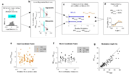
Fig 3 Estimating residual modulation 172
a, Example workflow for estimating residual modulation in coordinate frames irrelevant for neural
173
output that result from biases in head direction. Residual modulation was defined as: (MDIrrelevant / 174
MDRelevant). Estimations performed separately using simulated units for each behavioral session. b 175
Residual modulation was inversely correlated with standard deviation of head directions (σ). Red
11 / 57
filled lines indicate regression fit and confidence intervals. Dashed lines indicate data point for the
177
single session in (a).
178
179
Egocentric and allocentric tuning in auditory cortex 180
During exploration we recorded the activity of 186 sound-responsive units (50 single units, 181
136 multi-units) in auditory cortex (Supplementary Fig. 2). Electrode arrays were targeted to span 182
the low frequency areas where the middle and posterior ectosylvian gyral regions meet and thus 183
units were sampled from primary auditory cortex and two tonotopically organised secondary fields: 184
the posterior pseudosylvian and posterior suprasylvian fields. We analysed the firing rates of units in 185
the 50 milliseconds after the onset of each click; this window was wide enough to capture the neural 186
response while being sufficiently short that the animal’s head moved less than 1 cm (median 4 mm, 187
Supplementary Fig. 3) and less than 30° (median 12.6°) – the interval between speakers. The time 188
interval between stimuli always exceeded 250 ms. 189
We identified periods of time when the animal was facing forwards (± 15° of the arena 190
midline) at the center of the speaker ring (Supplementary Fig. 4): in this situation we mimic classic 191
neurophysiological investigations of spatial tuning in which head and world coordinate frames are 192
aligned. In the aligned case, we recorded 92 units that were significantly modulated by sound source 193
location (Fig 4a-d: Top left, GLM analysis of deviance, p ≤ 0.05) and for which spatial tuning curves 194
12 / 57 0.0131). We then compared the aligned control condition with all data when the head and world 196
coordinate frames were free to vary. Compared to the aligned condition, correlation between 197
egocentric and allocentric tuning curves when coordinate frames were free to vary was significantly 198
reduced (Fig 4e, R2 = 0.522 ± 0.0294) (paired t-test: free vs. aligned t91 = 8.76, p < 0.001) and 199
differences in spatial tuning in head and world coordinate frames became visible (Fig 4a-d: Bottom 200
left). 201
Fig 4 Spatial tuning of egocentric and allocentric units 202
a-d, Spatial tuning of four example units that were classified as egocentric (a-b) or allocentric (c-d).
203
In each panel, top left: Tuning curves calculated for sound angle in head and world coordinate frames
204
(CF) when both frames were aligned. Bottom left: Tuning curve when head and world CFs were free
205
to vary. Top and bottom right: Tuning curves plotted at specific head rotations. Model fit refers to
206
percentage of explainable deviance calculated according to Figure 6 across all data in which
207
coordinate frames were free to vary.Data for all tuning curves are shown as mean ± s.e.m. firing
208
rates. Dotted lines show the mean background activity measured in the 50 ms before stimulus
209
presentation. e, Correlation coefficients between tuning curves in head and world CFs when aligned
210
or free to vary as the animal foraged around the arena. Boxplots show median and inter-quartile range;
211
symbols show coefficients for individual units.
13 / 57 213
When animals moved freely through the arena, and head and world coordinate frames were 214
thus dissociated, we observed units consistent with egocentric (Fig 4a-b and Supplementary Fig. 5) 215
and allocentric hypotheses (Fig 4c-d and Supplementary Fig. 6). For units consistent with the 216
egocentric hypothesis, spatial receptive fields were more strongly modulated by sound angle in the 217
head than world coordinate frame. For the unit shown in figure 4a, modulation depth values in the 218
head and world coordinate frames were 28.3% and 10.1% respectively. In figure 4b, modulation 219
depth was 49.0% in the head coordinate frame and 30.3% in the world coordinate frame. 220
14 / 57 rotation but shifted systematically when plotted relative to the world (Fig 4a-b: Right columns). Both 222
outcomes are highly consistent with our simulation predictions (Fig 1). 223
In addition to identifying head-centered spatial tuning across movement, we also found 224
units with spatial tuning that realized the predictions generated by the allocentric hypothesis. These 225
units showed greater modulation depth to sound angle in the world coordinate frame than head 226
coordinate frame (Fig 4c-d and Supplementary Fig. 6): For putative allocentric units, modulation 227
depths for tuning curves were 21.2% and 13.4% in the world and head coordinate frames 228
respectively for the unit shown in Fig. 4c, and 12.7% and 10.1% respectively for the unit shown in 229
Fig. 4d. While these modulation depth values for these units were relatively low (possibly due to the 230
high background activity), their tuning curves were consistent with representations of world-231
centered sound location. Specifically for allocentric units, spatial tuning in the world coordinate 232
frame was robust to head rotation whereas tuning curves expressed relative to the head were 233
systematically shifted when mapped according to head direction (Fig 4c-d: Right column). 234
Modulation depth across coordinate frames 235
To quantify the observations we made above and systematically compare spatial tuning in 236
world and head coordinate frames, we calculated modulation depth for both tuning curves for each 237
unit. We next asked if modulation depth observed in either head or world coordinate frames was 238
greater than the residual modulation predicted by our earlier simulations (Fig.3b). A linear 239
regression model developed using simulated receptive fields was used to predict the magnitude of 240
residual tuning for each coordinate frame from the animal’s behavior during the recording of each 241
unit (Fig 5a-d). To describe the animal’s behavior across the relevant testing sessions for each neural 242
recording, we calculated the standard deviation of head directions (Fig. 5a). A smaller standard 243
deviation indicates a less uniform range of head-directions and when combined with our regression 244
model (Fig 5b) would predict higher residual modulation in both coordinate frames. Thus for a given 245
15 / 57 residual modulation in head and world coordinate frames arising from allocentric or egocentric 247
tuning respectively (Fig. 5c). The observed modulation values were calculated for each unit as the 248
ratio of modulation depth in one coordinate frame divided by the other coordinate frame (Fig. 5d) 249
and significance was attributed when test values exceeded the confidence interval of residual 250
[image:15.595.67.526.504.766.2]modulation. 251
Fig 5 Modulation depth across coordinate frames 252
a-d Workflow illustrating the use of animal behavior (a: summarized using the standard deviation of
253
head directions during neural testing, σ) and linear regression models (b – see also Fig 3) to generate
254
confidence intervals for residual modulation (c) that were compared to observed modulation depth
255
values (d) normalized relative to the alternative coordinate frame. Blue vertical lines in b show the σ
256
value in a. e-f, Normalized modulation depth observed for each spatially tuned unit compared against
257
the mean residual modulation predicted from behavior in head (e) or world (f) coordinate frames.
258
Bonferroni-corrected statistical criterion (p = 5.43 x 10⁻⁴) is denoted by . g, Modulation depth for all 259
spatially modulated units (n = 92) compared in world (MDWorld) and head coordinate frames (MDHead) 260
during exploration.
261
16 / 57 Across all spatially tuned units, modulation in the head coordinate frame was significantly 263
greater than predicted for 87 / 92 units (94.6%)(p < 0.05, Fig 5e); modulation in the world coordinate 264
frame was significant for 19 / 92 units (20.7%, Fig 5f). For 14 / 92 units (15.2%), modulation depth 265
was significantly greater than expected in both coordinate frames. When Bonferroni corrected for 266
multiple (n = 92, α = 5.43 x 10⁻⁴) comparisons these numbers dropped to 69 / 92 units (75%) for 267
modulation in the head coordinate frame, none of which were additionally modulated in a world 268
coordinate frame, and 6 / 92 units (6.5%) for modulation in the world coordinate frame – none of 269
which showed significant head-centered modulation. With this more conservative statistical 270
threshold, modulation depths were not significantly greater than expected in either coordinate 271
frame for the remaining 17 / 92 units (18.5%). Together these observations suggest that response 272
types occupy a continuum from purely egocentric to purely allocentric. The existence of units with 273
significant modulation in both coordinate frames with a less conservative statistical cut-off, or no 274
significant modulation with corrected threshold may indicate mixed spatial sensitivity comparable 275
with other reports in auditory cortex [23]. 276
A key prediction from our simulations with both uniform head-directions (Fig.1) and actual 277
head-directions (Fig 3a) was that modulation depth would be greater in the coordinate frame that 278
was relevant for neural activity than the irrelevant coordinate frame (i.e. Head > World for 279
egocentric; World > Head for allocentric). Having demonstrated that modulation within both co-280
ordinate frames was greater than expected based on the non-uniform sampling of head direction, 281
we compared the modulation depth across coordinate frames for all spatially tuned units (Fig 5g). 282
For 76 / 92 units (82.6%), we observed greater modulation depth in the head than world coordinate 283
frame indicating a predominance of egocentric tuning and a minority of units (16 / 92, 17.4%) in 284
17 / 57 General Linear Modelling to define egocentric and allocentric populations
286
Our analysis of modulation depth indicated the presence of both egocentric and allocentric 287
representations in auditory cortex but also highlighted that the analysis of modulation depth alone 288
was sometimes unable to resolve the coordinate frame in which units encoded sound location. To 289
calculate modulation depth requires we discretize sound location into distinct angular bins, average 290
neural responses across trials and thus ignore single trial variation in firing rates. General linear 291
models (GLMs) potentially offer a more sensitive method as they permit the analysis of single trial 292
data and allow us to treat sound angle as a continuous variable. We considered two models which 293
either characterized neural activity as a function of sound source angle relative to the head 294
(GLMHEAD) or in the world (GLMWORLD). For all units for which at least one GLM provided a statistically 295
significant fit (relative to a constant model, analysis of deviance; p < 0.05, 91 / 92 units), we 296
compared model performance using the Akaike information criterion (AIC)[24] for model selection. 297
In accordance with the modulation depth analysis, the majority of units were better modelled by 298
sound angle relative to the head than world (72/91 units; 79.1%; four animals) consistent with 299
egocentric tuning. However, we also observed a smaller number of units (19/91 units; 20.9%; three 300
animals) whose responses were better modelled by sound angle in the world and thus showed 301
stronger representation of allocentric sound location. 302
To visualize GLM performance and explore egocentric and allocentric tuning further, we 303
plotted a normalized metric of the deviance value usually used to assess model fit. Here we defined 304
model fit as the proportion of explainable deviance (Fig 6a) where a test model (e.g. GLMWORLD) is 305
considered in the context of GLMs that have no variable predictors of neural activity (a constant 306
model) or use sound angle in both coordinate frames as predictors (a full model). This normalization 307
step is critical in comparing model fit across units as deviance values alone are unbounded. In 308
contrast, model fit is limited from 0 (indicating the sound angle provides little information about the 309
18 / 57 neuron’s response as well as sound angles in both frames). While the units we recorded formed a 311
continuum in this space, for the purpose of further analysis we defined egocentric and allocentric 312
units according to the coordinate frame (head / world) that provided the best model fit as 313
determined by the AIC above. 314
Using a GLM based analysis, we predicted that egocentric units would have a high 315
percentage of the full model fit by sound angles relative to the head, and a low model fit for sound 316
angles relative to the world, and that allocentric units would show the reciprocal relationship. To 317
test these predictions we generated a model preference score; the model fit for sound angles 318
relative to the head minus the model fit for sound angles in the world. Accordingly, negative values 319
of model preference should identify allocentric units while positive values should indicate egocentric 320
units. Neurons in which both sound angles relative to the world and head provide high model fit 321
values may represent sounds in intermediary or mixed coordinate frames and would have model 322
preference scores close to zero, as would neurons in which we were unable to disambiguate 323
coordinate frame preference due to non-uniform head angle distributions. 324
Fig 6 General linear modelling of spatial sensitivity 325
a, Calculation of model fit for sound angle relative to the head or world. Raw deviance values are
326
normalized as a proportion of explainable deviance; the change in deviance between a constant and a
327
full model. b, Model fit comparisons for all units when the animal was free to move through the
328
arena. c, Model preference that indicates the distribution of units across the diagonal line of equality
329
in (b). d-e, Model fit and model preference for data when the head and world coordinate frames were
330
aligned. Grey background in (e) shows the distribution of model preference in the freely varying
331
condition for reference. f, Change in model fit between freely moving and aligned states for egocentric
332
and allocentric units in head and world coordinate frames. g-h, Model fit and model preference for
333
freely moving data when speaker identity was shuffled. Data points in (g) show for each unit the
334
median model fit averaged across 1000 shuffles. i, Change in model fit between unshuffled and
19 / 57
shuffled data. j-k, Model fit and model preference for freely moving data when the animal’s head
336
direction was shuffled. Data points in (j) show for each unit median model fit averaged across 1000
337
shuffles. l, Change in model fit between unshuffled and shuffled data. Asterisks with horizontal bars
338
in (f), (i) and (l) indicate significant interactions (two-way anova on change in model fit with shuffle)
339
between coordinate frame (head / world) and unit type (egocentric / allocentric) (p < 0.001). Asterisks
340
/ n.s. for each bar represent significant / non-significant effects of shuffle on model fit in specific
341
coordinate frames and for specific unity types (red/blue; t-test, p < 0.05).
342
20 / 57 In the space defined by model fit for sound angles relative to the head and world (Fig 6b), 344
units clustered in opposite areas supporting the existence of both egocentric and allocentric 345
representations. This clustering was also evident in the model preference scores, which showed a 346
bimodal distribution (Fig 6c). Repeating this analysis on data in which the head and world coordinate 347
frames were aligned (due to the animals position at the center of the speaker ring) demonstrated 348
that model fit values for head and world coordinate frames became more similar and model 349
preference scores were centered around zero (Fig 6d-e). When we compared the change in model fit 350
with alignment (two-way anova), this was reflected as a significant interaction between coordinate 351
frame (head or world) and unit type (egocentric or allocentric, determined by the coordinate frame 352
that provided best model fit using the AIC)(F1,178 = 130.1, p = 5.71 x 10⁻²³). Post-hoc comparison 353
confirmed that model fit in the head coordinate frame decreased significantly for egocentric units 354
(Bonferroni corrected for multiple comparisons, p = 5.04 x 10⁻⁵) and increased significantly for 355
allocentric units (p = 4.36 x 10⁻⁴). In contrast in the world coordinate frame, alignment led to a 356
significant increase in model fit for egocentric units (p = 2.22 x 10⁻²⁰) and a non-significant decrease 357
in model fit for allocentric units (p = 0.155). 358
We performed two additional control analyses on the freely moving dataset: firstly, we 359
randomly shuffled the speaker identity while maintaining the same information about the animal’s 360
head direction. Randomising the speaker identity should affect the ability to model both egocentric 361
and allocentric neurons and we would therefore predict that model fits for spatially relevant 362
coordinate frames would be worse and model preference scores would tend to zero. (I.e. shuffling 363
would shift model preference scores in the negative direction for egocentric units and the positive 364
direction for allocentric units). As predicted, shuffling speaker identity eliminated clustering of 365
egocentric and allocentric units in the space defined by model fit (Fig 6g) and lead to opposing 366
effects on model preference (Fig. 6h-i): Model fit scores for egocentric and allocentric units were 367
both affected by shuffling speaker identity but in opposite directions (unit x coordinate frame 368
21 / 57 relative to the head declined significantly with shuffling (p = 7.44 x 10-41) while fit for sound angle in 370
the world did not change significantly (p = 0.271). For allocentric units, model fit for sound angle in 371
the world declined significantly (p = 1.29 x 10⁻⁸) but was not significantly different in the head 372
coordinate frame (p = 0.35). When shuffling stimulus angle (averaging across 1000 shuffles), we 373
identified 12 / 19 (63.2%) allocentric and 63 / 72 (87.5%) egocentric units with model preference 374
scores beyond the 97.5% percentile limits of the shuffled distribution. 375
Secondly, we shuffled information about the animal’s head direction while maintaining 376
information about speaker identity. This should cause model fit values to decline for sound angle 377
relative to the head for egocentric units and should therefore result in egocentric units shifting their 378
model preference scores towards zero. For allocentric units the model fit for sound location in the 379
world should be maintained, and we would not predict a systematic change in model preference. 380
This was indeed the case (Fig 6j-l; interaction between coordinate frame and unit type: F1, 178 = 216.7, 381
p = 1.35 x 10⁻³²): For egocentric units shuffling head direction significantly reduced model fit in the 382
head coordinate frame (p = 1.40 x 10⁻²⁷) and increased model fit in the world coordinate frame (p = 383
2.20 x 10⁻³¹). For allocentric units, shuffling head direction did not significantly affect model fit in 384
either head (p = 0.211) or world coordinate frames (p = 0.178). 385
Egocentric and allocentric units – population characteristics 386
For egocentric units that encoded sound location in the head coordinate frame, it was 387
possible to characterize the full extent of tuning curves in 360° around the head (Fig 5a-b) despite 388
our speaker array only spanning 180°. This was possible because the animal’s head direction varied 389
continuously across 360° and so removed the constraints on measurement of spatial tuning imposed 390
by the range of speaker angles used. Indeed, we were able to extend our approach further to 391
characterize super-resolution tuning functions with an angular resolution more precise than the 392
interval between speakers (Fig 7a-b and Supplementary Fig 7). Together these findings show it is 393
22 / 57 greater detail than would be possible if the subject’s head position and direction remained constant 395
relative to the sound sources. Egocentric units shared spatial receptive field properties typical of 396
previous studies [15, 16, 18, 25]: units predominantly responded most strongly to contralateral 397
space (Fig 7c) with broad tuning width (Fig 7e-f) that typifies auditory cortical neurons. We also 398
found similar, if slightly weaker spatial modulation when calculating modulation depth according to 399
[image:22.595.76.522.468.725.2]Ref. [18] (Fig 7d). 400
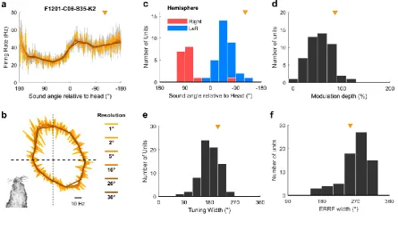
Fig 7 Egocentric unit characteristics 401
a-b, Spatial tuning of example egocentric unit at multiple angular resolutions. Data shown as mean ±
402
s.e.m. firing rate plotted in Cartesian (a) or polar (b) coordinates. Triangle indicates preferred location
403
of unit. Inset (b) illustrates the corresponding head direction onto which spatial tuning can be
super-404
imposed. c, Preferred location of all egocentric units (n = 72) in left and right auditory cortex. d,
405
Modulation depth calculated according to [18] across 360° for units in both hemispheres. e-f, Tuning
406
width (e) and equivalent rectangular receptive field width (ERRF)(f) for all units. Triangle indicates
407
the preferred location, modulation depth, tuning width and ERRF of the example unit in (a).
408
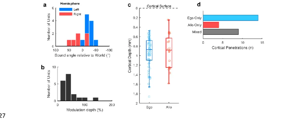
23 / 57 For allocentric units, we observed a similar contralateral tuning bias in preferred location 410
(Fig 8a) to egocentric units and that allocentric units had relatively low modulation depths (Fig 8b). 411
These tuning features may not be surprising as an allocentric receptive field could presumably fall 412
anywhere within or beyond the arena, and might therefore be poorly sampled by circular speaker 413
arrangements. If the tuning curves measured here were in fact sampling a more complex receptive 414
field that related to a world-centered coordinate frame (Fig 1b) we would predict that the receptive 415
fields would be correspondingly noisier. Allocentric and egocentric units were recorded at similar 416
cortical depths (Fig 8c) and on the same cortical penetrations as egocentric units were recorded on 9 417
[image:23.595.45.510.561.765.2]of 13 electrodes (69.2%) on which we also identified allocentric units (Fig 8d). 418
Fig 8 Allocentric unit characteristics 419
a, Preferred location of all allocentric units (n = 19) in left and right auditory cortex. b, Modulation
420
depth calculated across 180° for units in both hemispheres. c, Comparison of cortical depth at which
421
egocentric and allocentric units were recorded. Ferret auditory cortex varies in thickness between 1.5
422
and 2 mm and electrode depths were confirmed histologically (Supplementary Fig. 2). d, Number of
423
cortical penetrations on which we recorded only egocentric units, only allocentric units or a
424
combination of both (mixed). All 92 spatially tuned units were recorded on 27 unique electrodes, with
425
recorded units being distributed throughout cortex as the electrodes were descended.
426
24 / 57 Timing of spatial information
428
Our findings suggested the existence of egocentric and allocentric tuning in auditory cortex. 429
As these descriptions were functionally defined, we hypothesized that differences between 430
allocentric and egocentric tuning should only arise after stimulus presentation. To test this, we 431
analyzed the time course of unit activity in a moving 20 ms window and compared model fit and 432
model preference of egocentric and allocentric units (defined based on the AIC analysis above) using 433
cluster-based statistics to assess significance [26]. Model fit for sound angles relative to the head 434
was greater for egocentric than allocentric units only between 5 and 44 ms after stimulus onset (Fig 435
9a, p = 0.001996). Model fit for sound angles in the world was greater for allocentric than egocentric 436
units only between 6 and 34 ms after stimulus (Fig 9b, p = 0.001996). Model preference diverged 437
only in the window between 4 and 43 ms after stimulus onset (Fig 9c, p = 0.001996). We observed 438
no differences between egocentric and allocentric units before stimulus onset or when coordinate 439
frames were aligned (Supplementary Figure 8). Thus the differences between egocentric and 440
allocentric units reflected a stimulus-evoked effect that was only observed when head and world 441
coordinate frames were free to vary. 442
Fig 9 Egocentric and allocentric tuning over time 443
a, Model fit for predicting neural activity from sound angles relative to the head. b, Model fit for
444
predicting neural activity from sound angles in the world. c, Model preference. Data shown as mean ±
445
s.e.m. for egocentric and allocentric unit populations. Black lines indicate periods of statistical
446
significance (cluster based unpaired t-test, p < 0.05).
25 / 57 448
Population representations of space 449
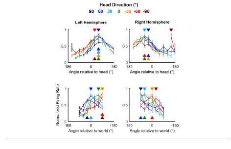
We next asked how auditory cortical neurons behaved as a population when spatial tuning 450
was compared across head directions. In contrast to individual units, population activity more closely 451
reflects the large-scale signals observed in human studies using electroencephalography (EEG) to 452
distinguish coordinate frame representations [11, 12]. To form populations, we took the unweighted 453
mean of normalized firing rates from all units recorded from left (n = 64) or right (n = 28) 454
hemispheres and compared tuning curves measured at different head directions. As would be 455
expected from the predominance of egocentric units, we found that tuning curves for both left and 456
right auditory cortical populations were consistent within the head but not world coordinate frame 457
26 / 57 population readouts of spatial tuning, potentially accounting for conflicting findings of coordinate 459
[image:26.595.56.529.265.569.2]frame representations from EEG recordings. 460
Fig 10 Auditory cortical tuning 461
Population tuning curves plotted across head direction for mean (± s.e.m.) normalized response of all
462
units in left and right auditory cortex; filled triangles indicate sound angle of maximum response at
463
each head direction.
464
465
Distance modulation of cortical neurons and spatial tuning 466
Studying auditory processing in moving subjects allowed us to resolve coordinate frame 467
ambiguity so that we could determine the spaces in which neurons represent sound location. 468
However recording in freely moving subjects also made it possible to go beyond angular 469
measurements of the source location and address how neurons represented the distance of sound 470
sources. Though often overlooked, distance is a critical component of egocentric models of neural 471
27 / 57 change as sound sources approach the head. For distant sound sources (typically > 1 m) ILDs are 473
small relative to distance-related attenuation of sound; however ILDs become much larger as sounds 474
approach the head and source-receiver distance decreases [27, 28]. Neurons must therefore 475
accommodate for distance dependent cues to accurately represent sound location across changes in 476
head position. In our study, the distance between head and sound source ranged from 10 cm (the 477
minimum distance imposed by the arena walls) to 40 centimetres, with only 3.37% of stimuli (mean 478
across 57 test sessions) presented at greater distances (Fig. 2g) and thus all stimuli were likely to 479
produce large ILDs [27, 28]. 480
Spatial tuning was observed at all distances studied in both egocentric (Fig 11a) and 481
allocentric units (Fig 11b) however modulation depth increased with distance for egocentric units 482
(ANOVA, F2,216 = 3.45, p = 0.0334). Pairwise post-hoc comparisons showed that modulation depth 483
was largest for sounds at greatest distances (Fig 11c) though the only significant difference was 484
found for sounds presented 20 to 30 cm and 30 to 40 cm away (t72 = -3.54, p = 0.0279). In contrast,
485
modulation depth did not change significantly with distance for allocentric units (Fig 11d, F2, 57 = 486
0.962, p > 0.1). 487
Fig 11 Spatial tuning across distance 488
a-b, Tuning curves of an egocentric (a) and allocentric (b) unit obtained with sound sources at
489
varying distances from the animal’s head. Bar plots show the number of stimuli and modulation depth
490
for each tuning curve. c-d Distributions of modulation depth measured across distance for egocentric
491
and allocentric units. Asterisk indicates significant pair-wise comparison (Tukey-Kramer corrected, p
492
< 0.05).
28 / 57 494
Speed modulation of cortical neurons and spatial tuning 495
Changes in head position and direction also allowed us to investigate how speed of head 496
movement (Fig. 2f) affected neural activity. Movement is known to affect auditory processing in 497
rodents [29-31] but its effects on spatial representations of sound location and also on auditory 498
cortical processing in other phyla such as carnivores remain unknown. Here we presented click 499
sounds for which dynamic acoustic cues would be negligible and thus we could isolate the effects of 500
head movement on neural activity. 501
To address auditory cortical processing first, we asked how many of our recorded units 502
(regardless of auditory responsiveness or spatial modulation) showed baseline activity that varied 503
with speed. For each unit, we took all periods of exploration (excluding the 50 ms after each click 504
onset) and calculated the speed of the animal at the time of each action potential. We then 505
discretized the distribution of spike-triggered speeds to obtain spike counts as a function of speed 506
and normalized spike counts by the duration over which each speed range was measured. This 507
process yielded a speed-rate function for baseline activity (Fig 12a). We then fitted an exponential 508
29 / 57 coefficients (β) of each curve to map the magnitude and direction of association between speed and 510
baseline activity (Fig 12c). Across the recorded population, we saw both positive and negative 511
correlations representing units for which firing rate increased or decreased respectively with speed. 512
However a significantly larger proportion of the population increased firing rate with speed across all 513
units (t-test vs. 0; t308 = 3.77, p = 1.97 x 10⁻⁴). This was also true if we considered only sound 514
responsive units (t267 = 5.15, p = 5.17 x 10⁻⁷) or only spatially tuned units (t91 = 4.12, p = 8.41 x 10⁻⁵). 515
Fig 12 Speed related auditory cortical activity and sensory processing 516
a Example calculation of speed-related modulation of baseline firing of one unit using reverse
517
correlation. b, Example speed-firing rate function summarized using regression (β) and correlation
518
(R2) coefficients for the same unit as (a). c, Population distribution of regression and correlation 519
coefficients showing the predominance of units with increasing speed-rate functions (β >0). d-e,
Peri-520
stimulus time histogram of sound evoked responses for units that were modulated by speed: In (d)
521
activity was enhanced as speed increased from 1 to 7 cm s-1 and decreased thereafter. In (e) firing 522
decreased with increasing speeds, although speed-related modulation was smaller relative to sound
523
evoked activity than (d). f, Box plots showing distributions (median and inter-quartile range) of
524
evoked firing rates in response to clicks across speed for all sound responsive units. g, Population
525
distribution of regression coefficients (β) and model fit (analysis of deviance p values) for all
sound-526
responsive units. Units for which speed was not a significant predictor of neural activity (p > 0.001)
527
denoted in grey. h, Spatial tuning curve for one unit for clicks presented at different head movement
528
speeds. i-k, Change in preferred location (i), modulation depth (j) and min / max firing rates (k)of
529
egocentric and allocentric units as a function of speed. Data for d-e and h-k shown as mean ± s.e.m.
30 / 57 531
We also observed speed-related modulation of sound-evoked responses in individual units 532
(Fig. 12d-e). For each individual unit, we characterized the relationship between head speed and 533
single trial firing rates (averaged over the 50 ms post-stimulus onset) using a general linear model 534
that measured both the strength (analysis of deviance p value) and direction (model coefficient, β) 535
of association. Positive β values indicated an increase in firing rate with increasing speed whereas 536
negative β values indicated a fall in firing rate with increasing speed. Thus the direction of the 537
relationship between firing rate and speed was summarized by the model coefficient, allowing us to 538
map the effects of movement speed across the population (Fig. 12f). For 199/268 sound-responsive 539
units (74.3%), speed was a significant predictor of firing rate (analysis of deviance vs. a constant 540
model, p < 0.001) however the mean coefficient value for movement sensitive units did not differ 541
significantly from zero (t199 = 0.643, p = 0.521). This suggests the sound-responsive population was 542
evenly split between units that increased or decreased firing with speed. We noted that a 543
significantly greater proportion of spatially modulated units (74/92, 80.4%) had sound evoked 544
responses that were sensitive to speed than units that were either not spatially modulated or for 545
31 / 57 χ2 = 3.96, p < 0.05). For those 74 spatially modulated and speed sensitive units, coefficients were
547
mostly larger than zero (mean ± s.e.m. = 2.73 x 10⁻⁵ ± 1.53 x 10⁻⁵) however this effect was not 548
statistically significant (t73 = 1.80, p = 0.076). For the remaining speed sensitive units, the mean 549
coefficients was closer to zero (mean ± s.e.m. = -5.02 x 10⁻⁶ ± 1.49 x 10⁻⁵). 550
Lastly, we asked if speed affected spatial tuning. Spatial tuning could be observed at all 551
speeds of movement in spatially tuned units (Fig. 12h) and the preferred locations of units did not 552
vary systematically with speed (Fig 12i). For neither egocentric nor allocentric units was there a 553
significant effect of speed in an ANOVA on preferred locations (egocentric: F5, 432 = 0.53, p = 0.753; 554
allocentric: F5, 108 = 1.53, p = 0.188). However we did observe significant changes in modulation 555
depth (Fig 12j) both for egocentric (F5, 432 = 4.91, p = 0.0002) and allocentric units (F5, 108 = 5.09, p = 556
0.0003), indicating that spatial modulation was greater when the head was moving fastest. Change 557
in modulation depth resulted from both a gradual suppression in minimum and enhancement in 558
maximum firing rates with speed (Fig 12k). However none of these changes in minimum or 559
maximum firing rate were significant in comparisons across speed (ANOVA with speed as main 560
factor, p > 0.5) indicating that it was only through the aggregative change in responses to both 561
preferred and non-preferred locations that modulation depth increased with speed. 562
Discussion 563
Here we have shown that by measuring spatial tuning curves in freely moving animals it is 564
possible to demonstrate the coordinate frames in which neurons define sound location. For the 565
majority of auditory cortical neurons, we found egocentric tuning that confirm the broadly held but 566
untested assumption that within the central auditory pathway sound location is represented in 567
head-centered coordinates. We also identified a small number of units with allocentric tuning, 568
whose responses were spatially locked to sound location in the world, suggesting that multiple 569
32 / 57 identified across different analyses, observed in several subjects and could be dissociated from 571
egocentric receptive fields recorded in the same behavioral sessions. Finally we explored the 572
dependence of neural activity and spatial tuning on sound source distance and the speed of head 573
movements, demonstrating that both factors can modulate firing rates and spatial tuning in auditory 574
cortex. 575
Our results show that an animal’s movement can be successfully tracked to measure head-576
centered egocentric tuning during behavior. While we used speakers placed at 30° intervals across a 577
range of 180°, we were nonetheless able to characterize spatial tuning of egocentric units around 578
the full circumference of the head (i.e. Fig. 7b). This illustrates the practical benefit of using moving 579
subjects to characterize head-centered spatial tuning as the animal’s head rotation generates the 580
additional variation in sound angle relative necessary to fully map azimuthal tuning with a reduced 581
number of sound sources. Furthermore, as the animal’s head direction was continuous, the stimulus 582
angle was also continuous and thus it was possible to measure spatial tuning at finer resolutions 583
than that of the speaker ring from which stimuli were presented. In contrast to egocentric tuning, 584
our ability to map allocentric receptive fields was limited by the speaker arrangement that only 585
sparsely sampled world coordinates (Fig 2a). This may in part explain the low number of allocentric 586
units in our population and denser sampling of the world may reveal unseen allocentric tuning – for 587
example in the 94 units we recorded that were not spatially modulated by sound locations in the 588
world that we tested. While a full 360° speaker ring may offer a minor improvement in sampling 589
density, the radial organization of the ring remains a suboptimal design for sampling rectangular or 590
irregular environments. To fully explore the shape of allocentric receptive fields will require denser, 591
uniform speaker grids or lattices in environments through which animals can move between sound 592
sources. 593
A notable property of egocentric units was the relationship between modulation depth of 594
33 / 57 largely be driven by changes in inter-aural level differences, although other auditory and
non-596
auditory cues can affect distance perception [32-36]. However modulation depth in our study was 597
lowest for proximal sounds when ILDs would be larger, and when other cues such as inter-aural time 598
differences remain relatively constant [27, 28]. Localization of nearby sound sources (< 1 m) is 599
possible for ferrets and humans [37, 38], though within the range of distances we considered here, 600
angular error of azimuthal localization in humans increases slightly as sounds approach the head 601
[37]. Thus our findings are consistent with human psychophysical performance but suggest larger 602
localization cues may not always produce better sound localization by neurons in auditory cortex. In 603
future it will be critical to validate our findings for sound sources at greater distances where sound 604
localization has been more widely studied. 605
In addition to recording many egocentric units, we also recorded a small number of 606
allocentric units, supporting the idea that auditory cortex represents sound location in multiple 607
coordinate frames [23] and parses an auditory scene into distinct objects [39, 40]. We believe this is 608
the first study to look for world-centered encoding of sound locations at the cellular level and thus 609
the units we recorded, while small in number, reflect a novel spatial representation in the auditory 610
system. 611
A key question is where allocentric units reside in cortex: Egocentric and allocentric units 612
were located on the same electrodes and cortical depths, in the primary and posterior regions of 613
auditory cortex. However, the low density of electrodes in our arrays, and their placement over a 614
low frequency border, prevented us from mapping the precise tonotopic boundaries necessary to 615
attribute units to specific cortical subfields [41]. Future use of denser sampling arrays may enable 616
cortical mapping in behaving animals and thus precise localization of allocentric units. We targeted 617
the low-frequency reversal between primary and posterior auditory cortex as these areas are likely 618
to be sensitive to inter-aural timing cues, and the animals involved in this work were also trained to 619
34 / 57 may correspond to part of the ‘what’ pathway in auditory processing whereas the anterior
621
ectosylvian gyrus may correspond to the ‘where’ pathway in which spatial tuning is more extensive 622
[43, 44]. It is thus likely that the coordinate frames represented in our population (where only 49% 623
of units were spatially sensitive) may be more ubiquitous in anterior regions of ferret auditory 624
cortex. Indeed given sensorimotor and cross-modal coordinate frame transformations are a key 625
feature of activity in parietal cortex [10], it is likely that allocentric representations exist beyond 626
auditory cortex. 627
While the observation of allocentric receptive fields in tonotopic auditory cortex is novel, the 628
existence of allocentric representations has been predicted by behavioural studies in humans [6, 13]. 629
Furthermore, coordinate transformations occur elsewhere in the auditory system [23, 45] and 630
behavioral movements can influence auditory subcortical and cortical processing [29, 30]. Perhaps 631
most importantly, vestibular signals are integrated into auditory processing already at the level of 632
the cochlea nucleus [46] allowing the distinction between self and source motion [22]. Auditory-633
vestibular integration, together with visual, proprioceptive and motor corollary discharge systems, 634
provides a mechanism through which changes in head direction can partially offset changes in 635
acoustic input during movement to create allocentric representations. At present it is unclear 636
whether allocentric representations require self-generated movement and it will be interesting to 637
test if world-centered tuning is present if head direction is systematically varied in stationary 638
animals. 639
It is also unclear how head position is also integrated into auditory processing. Positional 640
information within the medial temporal lobe (or its carnivore equivalent) is a leading candidate given 641
the connections between entorhinal and auditory cortex [47, 48]; however the functional 642
interactions between these areas and their potential contributions to allocentric processing remain 643
to be addressed. Another critical question relates to the visual (or other sensory) cues that animals 644
35 / 57 cells remap in different settings [49, 50] and that auditory cortex receives tactile and visual
646
information through multiple pathways [48, 51], it will be interesting to determine if changes in 647
visual / tactile environment affects tuning of allocentric receptive fields, and if so, what 648
environmental features anchor auditory processing. 649
Variation in the animal’s head position with movement also allowed us to study the effects 650
of head movement speed on auditory processing and spatial tuning. In contrast to other studies in 651
freely behaving animals that reported movement-related suppression of activity [29-31] we found 652
that neurons tended to fire more strongly when the head moved faster (Fig 12). One reason for this 653
difference may lie in the behavior measured: Other investigators have covered a diverse range of 654
actions including locomotion in which both the head and body move and self-generated sounds are 655
more likely. We only considered the head speed of an animal and did not track the body position 656
that would distinguish head movements from locomotion (which was relatively limited given the size 657
of the animal and the arena). It is thus likely that much of the variation in speed we observe is a 658
product of head movement during foraging without locomotion and thus with relatively little self-659
generated sound. The behavior of our subjects may therefore present different requirements for 660
auditory-motor integration that result in distinct neural effects. 661
We also observed that spatial modulation was also greater when the animal was moving 662
faster, which may be consistent with the sharpening of tuning curves during behavioral engagement 663
[15]. While sharpening of engagement-related spatial tuning was linked to a reduction in spiking 664
responses at untuned locations, we observed non-significant decreases in peak and minimum firing 665
rates (which together increased modulation depth) suggesting that the mechanisms underlying 666
speed-related modulation of spatial tuning may be subtly different. At the acoustic level, faster 667
movements provide larger dynamic cues [2, 3] that improve sound localization abilities in humans [3, 668
36 / 57 In summary, we recorded spatial tuning curves in auditory cortex of freely moving animals to 670
resolve coordinate frame ambiguity. We demonstrated many egocentric units representing location 671
relative to the head and a small number of allocentric units representing sound location relative to 672
the world. We also studied the role of distance and speed in auditory cortical processing. Together 673
our findings illustrate that auditory cortical processing of sound space may extend to multiple 674
coordinate frames and spatial dimensions such as azimuth and distance, as well as non-auditory 675
37 / 57 Methods
677
Ethics statement 678
All experimental procedures were approved by a local ethical review committee (AWERB; 679
University College London and The Royal Veterinary College, University of London) and performed 680
under license from the UK Home Office (Project License 70/7267) and in accordance with the 681
Animals (Scientific Procedures) Act 1986. 682
Simulated spatial receptive fields 683
Egocentric 684
Egocentric tuning described the relationship between spike probability (P) and sound source 685
angle relative to the midline of the subject’s head (𝜃𝐻𝑆) and was simulated in Matlab (MathWorks) 686
using a Gaussian function: 687
𝑃(𝜃) = 𝑎𝑒−(𝜃𝐻𝑆−𝑏)22𝑐2
689
( 1 ) 688
In the example shown in figure 1a, parameters (a = 1.044, b = 0° and c = 75.7°) were determined by 690
manual fitting to find values for which egocentric and allocentric tuning matched qualitatively. The 691
theta domain was between ±180° binned at 1° intervals and distance of sound sources was not 692
included in the simulation. 693
Allocentric 694
Allocentric tuning describes the relationship between neural output (reported here as spike 695
probability; P) and sound source position within the world measured in Cartesian (𝑥, 𝑦) coordinates. 696
Spatial tuning was simulated as the dot product of spike probability vectors returned from functions 697
38 / 57 𝑃(𝑥, 𝑦) = 𝑓(𝑥) ∙ 𝑓(𝑦) ( 2 ) 699
In figure 1b, logistic probability functions were used for both dimensions: 700
𝑓(𝑥) = 𝑒 −(𝑥−µ)𝑠
𝑠 (1 + 𝑒−(𝑥−µ)𝑠 )
2 701
( 3 ) 702
𝑓(𝑦) = 𝑒 −(𝑦−µ)𝑠
𝑠 (1 + 𝑒−(𝑦−µ)𝑠 )
2 704
( 4 ) 703
With µ = 1000 mm and s = 400 mm for the x-axis, and µ = 0 mm and s = 1000 mm for the y-axis. For 705
both axes, spike probability vectors were generated for domains between ± 1500 mm binned at 2 706
mm intervals. 707
Stimulus presentation, head pose and movement 708
The position and orientation of the subject’s head within the world was described as a 709
coordinate frame transform composed of a translation vector between origins (indicating the head 710
position) and a rotation matrix between axes (indicating the head direction). Stimuli were presented 711
on each time step of the simulation from each speaker in a ring at 10° intervals, 1000 mm from the 712
origin of the world coordinate frame. As the simulation was deterministic, each stimulus was 713
presented to static simulations only once to calculate the response. When simulating motion, a 714
‘pirouette’ trajectory was constructed in which the subject’s head translated on a circular trajectory 715
(radius = 50 mm; angular speed = 30° per time-step) while simultaneously rotating (angular speed = 716
10° per time-step) for 7200 stimulus presentations (Supplementary Video 2). For each stimulus 717
presentation, the stimulus angle was calculated relative to both the midline of the head and the 718
39 / 57 Animals
720
Subjects were five pigmented female ferrets (1-5 years old) trained in a variety of 721
psychophysical tasks that did not involve the stimuli presented or the experimental chamber used in 722
the current study. Each ferret was chronically implanted with Warp-16 microdrives (Neuralynx, MT) 723
housing sixteen independently moveable tungsten microelectrodes (WPI Inc., FL) positioned over 724
middle and posterior fields of left or right auditory cortex. Details of the surgical procedures for 725
implantation and confirmation of electrode position are described elsewhere[54]. The weight and 726
water consumption of all animals was measured throughout the experiment. Regular otoscopic 727
examinations were made to ensure the cleanliness and health of ferrets’ ears. 728
Subjects were water-restricted prior to testing, during which they explored the experimental 729
arena to find freely available sources of water. On each day of testing, subjects received a minimum 730
of 60ml/kg of water either during testing or supplemented as a wet mash made from water and 731
ground high-protein pellets. Subjects were tested in morning and afternoon sessions on each day for 732
up to three days in a week (i.e. a maximum of six consecutive testing sessions); on the remaining 733
weekdays subjects obtained water in performance of other psychophysical tasks. Test sessions 734
lasted between 10 and 50 minutes and were ended when the animal lost interest in exploring the 735
arena. 736
737
Experimental Design and Stimuli 738
In each test session, a ferret was placed within a D-shaped arena (Fig. 2a, rectangular 739
section: 35 x 30 cm [width x length]; semi-circular section: 17.5 cm radius; 50 cm tall) with seven 740
speakers positioned at 30° intervals, 26 cm away from a central pillar from which the animal could 741
find water. The periphery of the circular half of the arena was also fitted with spouts from which 742