Synchronization of micromasers

C. Davis-Tilley and A. D. Armour

Centre for the Mathematics and Theoretical Physics of Quantum Non-Equilibrium Systems and School of Physics and Astronomy,

University of Nottingham, Nottingham NG7 2RD, UK

(Dated: November 15, 2016)

We investigate synchronization effects in quantum self-sustained oscillators theoretically using the micromaser as a model system. We use the probability distribution for the relative phase as a tool for quantifying the emergence of preferred phases when two micromasers are coupled together. Using perturbation theory, we show that the behavior of the phase distribution is strongly depen-dent on exactly how the oscillators are coupled. In the quantum regime where photon occupation numbers are low we find that although synchronization effects are rather weak, they are nevertheless significantly stronger than expected from a semiclassical description of the phase dynamics. We also compare the behavior of the phase distribution with the mutual information of the two oscillators and show that they can behave in rather different ways.

I. INTRODUCTION

Self-sustained oscillators do not have a preferred phase, but when two or more of them are weakly coupled to-gether a phase preference can emerge spontaneously, an effect known as synchronization. Self-sustained oscilla-tors are ubiquitous in nature and synchronization effects have been widely studied across the physical and biolog-ical sciences [1]. Synchronization has also been studied in quantum optical systems such as the laser, although generally focussing on regimes where approximate semi-classical descriptions work well [2, 3]. In the last few years there has been considerable interest in studying the synchronization of oscillators and related systems [4– 22] close to threshold or at low excitation levels where semiclassical approaches break down and fully quantum mechanical calculations are required. Recent theoretical work has explored different ways of quantifying synchro-nization in quantum oscillators [5, 7, 14, 15, 20], as well as investigating the connection between it and measures of correlation such as mutual information and entangle-ment [5, 8, 10, 15, 19]. Detailed comparisons have also been made between the predictions of quantum mod-els and those of related semiclassical or classical descrip-tions [7, 12].

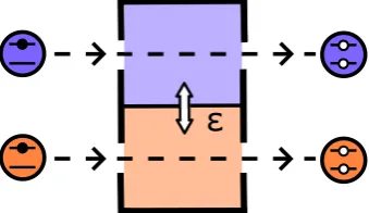
Studies of synchronization effects in the quantum regime have largely concentrated on the behavior of sim-ple model systems such as van der Pol oscillators [7, 9, 10, 12, 15, 17, 19, 21] (together with closely related models [22]), though a number of other systems includ-ing atomic ensembles [13, 16] and optomechanical oscil-lators [5, 6, 12, 18] have also been investigated. In this article we investigate synchronization in a very different model system consisting of two weakly coupled micro-masers (see Fig. 1).

The micromaser is a self-sustained oscillator consisting of a microwave cavity driven by a steady flow of excited atoms which interact strongly with a particular cavity mode [23–25]. The micromaser was used to carry out a range of pioneering experiments in quantum optics [23]. However, it has also become possible to engineer

sys-ε

FIG. 1: (Color Online) Schematic diagram of the coupled micromaser system. Each micromaser consists of an optical cavity which interacts with a flow of excited two-level atoms. If the cavities were separated by a partially reflecting mir-ror, photon tunnelling would lead to a (coherent) coupling between them,ε.

tems with similar behavior in the solid-state using, for example, superconducting [31, 32] or optomechanical [33] devices.

The micromaser makes a very interesting model sys-tem with which to explore synchronization effects in the quantum regime because it displays a very rich range of dynamical behaviors, including strongly non-classical features which go well beyond those found in simpler sys-tems like the quantum van der Pol oscillator. Further-more, an exact steady-state solution is available for the density operator of the micromaser [24] and important dynamical properties such as the linewidth [27–30] have been studied extensively.

it with numerical calculations using the full master equa-tion of the system. We find that whilst the Fokker-Planck equation provides a good description of the phase distri-bution in the semiclassical regime, it substantially under-estimates the extent to which a preferred phase emerges in the quantum regime. We also compare the behavior of the phase distribution with the mutual information and entanglement of the micromasers and find that the behavior is somewhat different in each case.

This work is organized as follows. We introduce our model of the coupled micromaser system and briefly re-view the key properties of the uncoupled micromaser in Sec. II. Then we introduce the relative phase distribution in Sec. III. We show how perturbation theory can be used to understand the behavior of the phase distribution in the weak coupling limit in Sec. IV. Then in Sec. V we de-rive a simple analytic formula for the phase distribution in the semiclassical limit and compare it with numerical calculations. We examine the behavior of other mea-sures of correlation between the micromasers in Sec. VI. Finally, we summarize our findings and discuss possible directions for future work in Sec. VII.

II. MICROMASER MODEL

We consider a model system consisting of two micro-masers, assumed for simplicity to be identical, that are coupled together weakly. As is the case for classical os-cillators [1, 34, 35], the behavior can be very sensitive to the form of the coupling as well as its strength. We investigate two specific forms for the coupling involving either additional terms in the Hamiltonian of the sys-tem (coherent coupling) or additional dissipative terms in the master equation (dissipative coupling). The start-ing point for our model is the standard master equation description for the micromaser [24, 25], to which we shall simply add additional terms to describe the coupling.

The master equation for the density operator of the two micromasers,ρ, (in the interaction picture) takes the form

˙

ρ=L1[ρ] +L2[ρ] +Lc[ρ] (1)

where here L1[ρ] and L2[ρ] describe the uncoupled dy-namics of the two micromasers and the interaction be-tween them is given byLc[ρ].

The dynamics of each individual micromaser is con-trolled by a balance of interactions between the cavity and the flow of atoms which pass through it, and be-tween the cavity and its electromagnetic environment which gives rise to losses. The atoms can be traced out of the master equation so that the dynamics of the system

is captured by the terms [24, 25]

Lj[ρ] = N

cos(φ

q

aja†j)ρcos(φ q

aja†j) (2)

+

a†_jsin(φ

q

aja†j) q

aja†j ρ

sin(φ

q

aja†j)aj q

aja†j

−ρ





+1 2

h

2ajρa†j−a †

jajρ−ρa†jaj i

,

whereajis the lowering operator for a mode of the cavity j (j = 1,2), N is the rate at which atoms pass through the cavity andφ is the Rabi angle which quantifies the strength of the atom-cavity interaction. Note that we have adopted units of time such that the cavity loss rate, γ, is unity and we have taken the zero-temperature limit for simplicity.

For coherent coupling between the two micromasers the interaction is described by the Hamiltonian

Hc=~ε(a1a†2+a †

1a2), (3) withεthe coupling strength (scaled by γ), and hence in this case

L(coh) c [ρ] =−

i

~

[Hc, ρ]. (4)

For dissipative coupling the master equation includes terms which describe an additional loss channel for the system whose properties depend on the state of both modes [10, 12, 17]

L(diss)

c [ρ] = ε h

(a1−a2)ρ(a†1−a † 2)

−1 2

n

(a†₁−a†₂)(a1−a2), ρo

. (5)

In the following we will focus mainly on the regime where the coupling is very weakε1.

Coherent coupling between two micromasers could be achieved by forming the cavities with a common mir-ror which is only partially reflective [26] (see Fig. 1) and would therefore allow photons to tunnel between the two cavities. Dissipative coupling might be engineered using a more elaborate set-up involving a third cavity placed between the cavities of the micromasers so that pho-tons can tunnel between it and each of the micromasers. An effective dissipative coupling between the micromaser cavities would then arise provided the third cavity was much more strongly damped, as discussed in Ref. 12.

Before going on to look at how either coherent or dissi-pative coupling affects the system, we briefly review the most important properties of the uncoupled micromaser (ε = 0). The steady-state density operator for a micro-maser is diagonal in the number state representation and the probability of finding the cavity in then-th number state is [24, 25]

Pn =K n Y

m=1

Nsin2(φ√m)

0 2 4 6 8 1 0 0 .2

0 .4 0 .6 0 .8 1 .0

⟨

n

⟩

/N

n

N = 5

N = 2 0

N = 5 0

0 2 4 6 8 1 0 0

1 0 2 0 3 0

0 .0 0 .2 0 .4 0 .6 0 .8 1 .0

Pn

0 2 4 6 8 1 0

1 2 3 4 5 6 7 8

F

N = 5

N = 2 0

N = 5 0 (a)

(b)

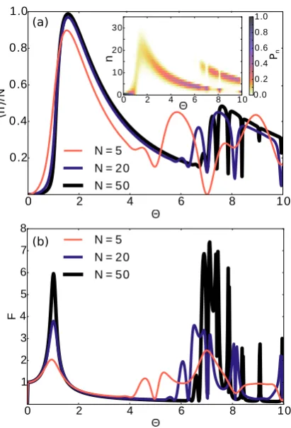
FIG. 2: (Color Online) Steady-state occupation number hni/N(a) and associated Fano factor,F, (b) for an uncoupled micromaser as a function of Θ =φN1/2 andN. The inset in (a) shows the full number distributionPn for the case where N= 20.

whereK is a constant determined by normalization. Although the density operator can be written in terms of an apparently simple formula, the state of the system changes dramatically as a function of the atomic flow rate,N, and the strength of the atom-cavity interaction, parameterized by the pump parameter: Θ =φN1/2_{. Fig.} 2 illustrates the behavior of the average occupation num-ber hni and the number fluctuations, measured by the Fano factor F = (hn2_{i − hni}2_{)/hni, as a function of Θ} and N; the inset shows an example of the full number distributionPn. The system has a threshold at Θ = 1, above which a limit-cycle emerges—manifesting in the Pn distribution as a peak at non-zeron. After initially growing very rapidly in size, the limit-cycle then gets progressively smaller as Θ is increased (up until Θ∼4). There is a strong peak inF around threshold and it then drops below unity, a signature of number squeezing [36]. For Θ>4 the behavior becomes more complicated and the micromaser moves between a range of different states. It undergoes dynamical transitions between limit-cycles with different average energies [24] and can co-exist in a mixed state involving two limit-cycle states (seen as two peaks in thePn distribution). At certain specific values ofφsuch that sin(φ√m+ 1) = 0 withm= 0,1,2, ...the

system becomestrapped: P(n>m)= 0 because the matrix element that generates transitions between the m and m+ 1 number states vanishes. These trapping states [23] have a number state distribution that can be extremely sharply peaked. For example, at φ = π/√2 (m = 1 trapping state) one typically finds P1 P0 and as N is increased the system gets closer and closer to being exactly in then= 1 number state.

The extremely narrow Pn distributions that the mi-cromaser displays above threshold come close to reaching what might be thought of as the most quantum of limit-cycle states—pure number states. However, the micro-maser’s steady-state isn’t always strongly non-classical. The average occupation number of the micromaser is roughly proportional to N for fixed Θ and the non-classical features are strongest for either relatively small N or larger values of Θ. In contrast, when hni 1 and hni φ2_{the dynamics of the number distribution,P}

n, is well described by a Fokker-Planck equation in whichnis treated as a continuous variable [24], which corresponds to the semiclassical limit of the system.

III. RELATIVE PHASE DISTRIBUTION

Phase distributions provide a convenient way of char-acterizing the emergence of a preferred relative phase in systems of coupled oscillators. For a single oscillator the quantum mechanical phase distribution is given by [36],

P(ϕ) = 1

2πhϕ|ρ|ϕi= 1 2π

∞ X

n,m=0

hn|ρ|miei(m−n)ϕ, (7)

where |ϕi = P∞ n=0e

inϕ_{|ni is an eigenstate of the} Susskind-Glogower operatorP∞

n=0|nihn+ 1|. This phase distribution,P(ϕ), also emerges naturally from the Pegg-Barnett description of the phase operator [37] or indeed when one seeks to define a distribution which is the canonical conjugate of the number distribution [38]. In the steady-state only the diagonal components of the un-coupled micromaser density operator are non-zero in the number distribution, so we see immediately that there is no preferred phase and the phase distribution is simply uniform: P(ϕ) = 1/2π.

When two micromasers are coupled, either coherently or dissipatively, a preference emerges for certain values of therelative phase,ϕ−=ϕ1−ϕ2, but not the total phase ϕ+=ϕ1+ϕ2. The relative phase distribution takes the form [14, 39, 40]

P(ϕ−) = 1 2π

∞ X

n,m=0 ∞ X

k=max(n,m)

eiϕ−(m−n)

×hn, k−n|ρ|m, k−mi, (8)

which can also be rewritten explicitly as a Fourier series

P(ϕ−) = 1 2π+

1 πRe

"_∞ X

p=1 eipϕ−

∞ X

n=0,m=0 ρ(_n,mp)

#

0 .0 0 .1 0 .2 0 .3 0 .4 0 .5 0 .0

0 .5 1 .0 1 .5

S

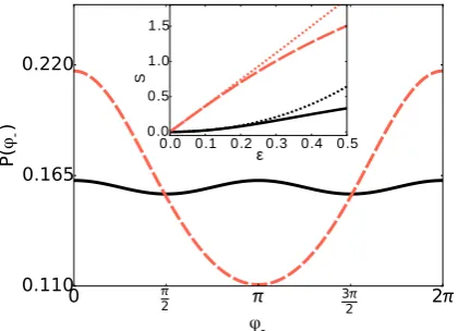
FIG. 3: (Color Online) Comparison of the relative phase probability distributions calculated numerically for coherent (solid, black) and dissipative (dashed, red) coupling with

ε = 0.1, N = 5 and Θ = φN1/2 _{= 2. The inset shows} the strengths of the peaks in the relative phase distributions, characterized byS, as a function of the coupling; the dotted lines are from the perturbation theory described in Sec. IV.

where we adopt the notationρ(n,mp) =hn, m+p|ρ|n+p, mi. It is also helpful to be able to characterize the emer-gence of a phase preference using a single number. Start-ing from the relative phase distribution, one can simply extract the size of the peak relative to the uniform dis-tribution [14],

S= 2πmax [P(ϕ−)]−1. (10)

This is something that we will make extensive use of here, though it should be noted that the choice is by no means unique [18, 22].

The relative phase distribution for the micromaser system is obtained by solving for the steady-state of the master equation (1) using standard numerical meth-ods [41]. Coherent and dissipative couplings with the same strength give rise to markedly different behavior in the relative phase distribution, as is illustrated in Fig. 3. Coherent coupling leads to much weaker phase locking than dissipative coupling and generates a relative phase distribution which isπ-periodic rather than 2π-periodic. This matches the well-known differences in relative phase dynamics of reactively and dissipatively coupled classical oscillators which are usually understood by deriving ap-proximate equations of motion for the relative phase of the oscillator assuming weak coupling [1, 35].

IV. PERTURBATION THEORY

Perturbation theory provides a straightforward way of understanding the differences between the quantum me-chanical relative phase distributions generated by coher-ent and dissipative coupling. We begin by considering the

case of coherent coupling before moving on to dissipative coupling.

A. Coherent Coupling

Writing the master equation in terms of the number state basis, we find

˙

ρ(_n,mp) = − "

µ(np)+µ (p) m

2 +c

(p) n +d

(p) n +c

(p) m +d

(p) m

#

ρ(_n,mp)

+c(_n−p)₁ρ_n−(p)_1,m+c(_m−p)₁ρ_n,m−(p) ₁+d(_np₊₁) ρ(_np₊₁) _,m

+d(_mp)₊₁ρ_n,m(p) ₊₁+ ∆(_n,mp) , (11) where the terms arising from the coupling are given by

∆(_n,mp) = −iεhpn(m+p+ 1)ρ(_n−p+1)_1,m

+p(n+ 1)(m+p)ρ(_np−₊₁1)_,m −pm(n+p+ 1)ρ(_n,m−p+1)₁

−p(n+p)(m+ 1)ρ(_n,mp−1)₊₁i, (12)

and the coefficients which describe the uncoupled evolu-tion are given by [27]

1 2µ

(p)

n = 2Nsin 2

_φ

2

_p

n+p+ 1−√n+ 1

+hn+p 2 −

p

n(n+p)i (13)

c(_n−p)₁ = Nsin(φ√n) sin(φ√n+p) (14) d(_np) = pn(n+p). (15)

In the steady-state ˙ρ(n,mp) = 0, leading to a set of linear equations for the componentsρ(n,mp) . Forε= 0 the sets of linear equations for differentpvalues are uncoupled; they are also homogeneous and have the solutionsρ(n,mp) = 0, except in the diagonal case (p= 0) where the components must also obey the normalization condition.

Working to first order in the coupling means that we replace the terms in Eq. (12) by their unperturbed val-ues which are all zero—apart from the diagonal ones, ρ(0)n,m=PnPm. Therefore only the equations for thep= 1 components are affected (we only need consider the com-ponents with p > 0 which appear in the expression for the relative phase distribution (9)) for which we find

∆(1)_n,m=−iεp(n+ 1)(m+ 1) (Pn+1Pm−Pm+1Pn). (16) Thus at first order, the componentsρ(1)n,m are in general non-zero, and pure imaginary (sincePn(m)are probabili-ties), whilst those withp >1 remain zero. However, since ∆(1)n,m=−∆

(1)

Working to second order in the coupling, ∆(2)n,m is no longer zero (sinceρ(1)n,m is of orderε) and one finds that the componentsρ(2)n,m are all real and proportional toε2. In this case there is no cancelling of the terms in the sum and hence to second order the relative phase distribution takes the form

P(ϕ−) = 1 2π

1 +ε2C0cos(2ϕ−), (17)

whereC0is a constant which depends on the parameters of the uncoupled micromasers (φandN). This of course is just what we see for the case of coherent coupling in Fig. 3.

B. Dissipative coupling

We now look at what happens for dissipative coupling described by Eq. (5). In this case we can simplify the master equation by taking into account the fact that some of the terms in (5) simply act to increase the effective damping of the oscillators and can be absorbed into the terms which are already present for the uncoupled system by rescaling the parameters: ˜N =N/(1+ε), ˜ε=ε/(1+ε). Working in the number basis, the master equation with dissipative coupling takes the form given by (11) (though with ˜εand ˜N replacingεandN) with

∆(n,mp) = −ε˜ hp

(n+ 1)(m+ 1)ρ(_np−₊₁1)_,m+1

+p(n+p+ 1)(m+p+ 1)ρ(_n,mp+1)

−1 2

p

n(m+p+ 1)ρ(_n−p+1)_1,m

−1 2

p

(n+p+ 1)mρ(_n,m−p+1)₁

−1 2

p

(n+ 1)(m+p)ρ(_np−₊₁1)_,m

− 1 2

p

(n+p)(m+ 1)ρ(_n,mp−1)₊₁

. (18)

At first order in the coupling, only the p = 1 term is non-zero,

∆(1)_n,m = ε˜ 2

p

(n+ 1)(m+ 1) (19)

×[Pn+1Pm+PnPm+1−2Pn+1Pm+1].

This generates non-zero componentsρ(1)n,m which are all real with ρ(1)n,m =ρ

(1)

m,n so there is no cancellation when they are summed up. Hence to lowest order in the pling the relative phase distribution for dissipative cou-pling takes the form

P(ϕ−) = 1

2π[1 +εC1cos(ϕ−)], (20) where C1 is a constant (that again depends on the pa-rameters of the uncoupled micromasers) which matches the behavior in Fig. 3.

The insights into the general form of the relative phase distribution provided by perturbation calculations are quite general, in the sense that the overall form of the relative phase distribution is entirely determined by the coupling terms (only the constantsC0andC1depend on the details of the micromaser systems). However, pertur-bation theory is also very useful for exploring the behav-ior where the state space of the system becomes so large that a direct numerical solution becomes impracticable.

V. SEMICLASSICAL LIMIT

To understand the behavior in the semiclassical limit we start from the expression for the relative phase dis-tribution in the form of Eq. (9) and focus on the case of dissipative coupling, which is the simplest. The equation of motion for the relative phase is given by

˙

P(ϕ−, t) = 1 πRe

"_∞ X

p=1 eipϕ−

∞ X

n,m=0 ˙ ρ(_n,mp)

#

. (21)

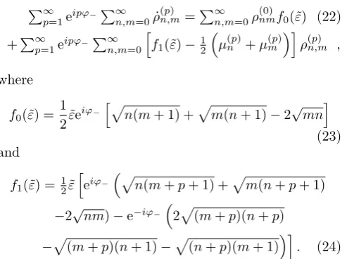
Using the master equation (11), with the dissipative cou-pling terms (18), we find that [29]

P∞ p=1eipϕ−

P∞ n,m=0ρ˙

(p)

n,m=P∞n,m=0ρ (0)

nmf0(˜ε) (22) +P∞

p=1e

ipϕ−P∞ n,m=0

h

f1(˜ε)−1 2

µ(np)+µ(mp) i

ρ(n,mp) ,

where

f0(˜ε) = 1 2ε˜e

iϕ−hp_{n(m+ 1) +}p_{m(n+ 1)−2}√_mni

(23) and

f1(˜ε) =1₂ε˜

h

eiϕ− _p

n(m+p+ 1) +pm(n+p+ 1)

−2√nm)−e−iϕ−

2p(m+p)(n+p)

−p

(m+p)(n+ 1)−p

(n+p)(m+ 1)i. (24)

Our assumptions mean that we need only consider the components ρ(n,mp) for which n, m p. We proceed by expanding the coefficients in (22) treatingp/n,p/m, 1/n and 1/mas small quantities and keeping the lowest order (non-zero) contributions in each case so that we have

f0(˜ε) ' 1 4ε˜e

iϕ−

_n+m √

nm

(25)

f1(˜ε) ' 1 4ε˜

eiϕ−_{(p+ 1) + e}−iϕ−_(p−1)

×

_n+m √

nm

(26)

and

µ(_np) '

4 ˜Nsin2

_pφ

4√n+ 1

+ p 2 4n

' "

˜ N p2_φ2 4(n+ 1) +

p2 4n

#

. (27)

In the last line we also expanded the sine assuming (pφ)2_/n1.

Finally, we make use of the assumption that the dis-tributions are strongly peaked about a common aver-age [27, 29] and simply replace n and m (together with n+ 1 andm+ 1) withhniso that now Eq. (22) takes the simplified form

∞ X

p=1 eipϕ−

∞ X

n,m=0 ˙

ρ(_n,mp) = 1 2ε˜e

iϕ−₋

∞ X

p=1 eipϕ−

∞ X

n,m=0 ρ(_n,mp)

×hp2∆˜ −ε˜(cosϕ−+ipsinϕ−) i

,

(28)

where we have defined

˜ ∆ =

˜ N φ2_{+ 1}

4hni . (29)

The parameter ˜∆ matches a simple approximate expres-sion for the micromaser linewidth [27–30] which is valid in the semiclassical regime.

Combining Eq. (28) with its complex conjugate leads to a Fokker-Planck equation for the relative phase distri-bution:

˙

P(ϕ−) = _∂

∂ϕ− ˜

εsinϕ−+ ˜∆ ∂2 ∂ϕ2

−

P(ϕ−). (30)

The corresponding steady-state distribution is [42]

P(ϕ−) = 1 2πI0(˜ε/∆)˜ e

˜

εcosϕ−/∆˜_{. (31)}

The Fokker-Planck equation for the phase distribution of the coupled micromasers is exactly what we would ex-pect for coupled classical oscillators in the presence of noise [1, 42]: it describes a competition between phase

diffusion and the effects of the coupling which tends to drive the system towards a particular relative phase. However, the origin of the noise which drives the diffusion is nevertheless ultimately quantum mechanical rather than classical and hence it makes sense to see (31) as a semiclassical equation in this context. It is worth not-ing that a Fokker-Planck equation with the same form emerges in the analysis of coupled lasers far above thresh-old [3].

Now that we have obtained an expression for the phase distribution in the semiclassical limit we can look in de-tail at when and how its predictions differ from the full (quantum) dynamics predicted by the master equation. The phase distribution obtained using the semiclassical approximation (31) is compared with the results from a full numerical solution of the master equation for a rel-atively small pumping rate,N = 5, in Fig. 4. The first thing to note is that the standard expectation of classical synchronization theory is fulfilled: for the weak couplings used here a rather strong change in the phase distribu-tion is combined with a relatively weak change in the average occupation number of the system. Furthermore, the semiclassical phase distribution does a reasonable job of describing the strength of the peak in the phase dis-tribution for Θ values that are not far above threshold. However, the semiclassical calculation systematically un-derestimates the strength of the phase locking in the quantum regime where hni ∼ 1 (i.e. Θ > 3) as shown in the inset to Fig. 4a. Although the phase locking is pretty weak for larger values of Θ, it is nevertheless about twice as strong as predicted by the simple semiclassical calculation.

Although a full numerical solution of the master equa-tion becomes very difficult for largerN values we can use perturbation theory to calculate the relative phase dis-tribution provided that we choose a small enough value for the coupling (since it turns out that the range of cou-pling strengths over which the second order perturbation calculation is a good description varies withN). Fig. 5 compares the value ofSobtained using the perturbation and semiclassical calculations for a range of N values. It shows clearly that the semiclassical solution (31) pro-vides an increasingly accurate description of the strength of the phase locking asN is increased, just as one would expect.

VI. MUTUAL INFORMATION AND ENTANGLEMENT

0 1 2 3 4 5 6 0.0

0.1 0.2 0.3 0.4 0.5 0.6 0.7

S

= 0.01 = 0.05 = 0.1

= 0.01 = 0.05 = 0.1

1 2 3 4 5 6

0 1 2 3 4 5 6

(a)

(b)

0.0 0.2 0.4 0.6 0.8 1.0

⟨

n

⟩

/N

0.2 0.0 0.2 0.4 0.6

(1

-S

S

C

/S

)

= 0.01 = 0.05 = 0.1

FIG. 4: (Color Online)(a) Strength of the relative phase lock-ing, measured by S = 2π[P(ϕ−)max]−1, as a function of Θ =φN1/2 _{for dissipative coupling withN= 5 andε= 0.01,} 0.05 and 0.1. In each case the results of full numerical calcu-lations are shown as full lines and the results from a semiclas-sical calculation using the Fokker-Planck equation are dotted lines. The inset shows the relative difference between the quantum and semiclassical calculations for the same param-eters. [Note that the small peak around Θ = 5 corresponds to the n = 1 trapping state.] (b) Behavior of the average photon number for the same parameters compared with the uncoupled case,ε= 0 (dotted line).

suggested that mutual information could serve as an or-der parameter for synchronization [15].

The mutual information,I, of the coupled micromasers is defined as

I=S(ρ1) +S(ρ2)− S(ρ), (32)

whereρis the full density operator,ρ1(2), is the reduced density operator of micromaser 1(2) and S is the von Neumann entropy,S(ρ) =−Tr[ρlnρ].

Perturbation theory tells us immediately that the mutual information of micromasers will grow at least quadratically with the strength of the coupling, for both dissipative and coherent coupling. To see this, we can write the density operator ρ, its eigenvalues λj, and

1 2 3 4 5 6

0.2 0.1 0.0 0.1 0.2 0.3 0.4 0.5 0.6

1

-S

S

C

/S

p

e

rt

N = 5 N = 20 N = 50 N = 100

Θ

FIG. 5: (Color Online) Relative difference between the quan-tum (perturbation theory) and semiclassical calculations of the strength of the phase locking,S, for different values ofN

withε= 0.0001.

eigenkets|ji, as expansions in [43]ε

ρ = ρ(0)+ερ(1)+. . . (33) λj = λ0j+ελ1j +. . . (34) |ji = |j(0)i+ε|j(1)i+. . . (35)

To first order, the von Neumann entropy is

S(ρ) =S(ρ(0))−εX j

λ(1)_j 1 + lnλ(0)_j , (36)

with λ(1)_j =hj(0)|ρ(1)|j(0)i, the first order correction to the eigenvalues. The density operators for uncoupled mi-cromasers are diagonal in the number state basis,

ρ(0)=X n,m

PnPm|n, mihn, m|, (37)

and as we have seen in Sec. IV the first order correction terms which form ρ(1) _{are all off-diagonal in the} num-ber state basis; consequently the first order corrections to the eigenvalues are all zero. Hence the first order con-tributions toI vanish for both coherent and dissipative couplings.

Fig. 6 compares the behavior of the mutual informa-tion for dissipative and coherent couplings. Not only doesI grow quadratically withε in both cases, but the magnitudes are very similar. This is in sharp contrast to the behavior of the relative phase distributions where the dissipative coupling leads to much stronger features inP(ϕ−) than the coherent coupling [see Fig. 3], with a linear rather than a quadratic dependence onε.

0 .0 0 .2 0 .4 0 .6 0 .8 1 .0

ε

0 .0 0 .2 0 .4 0 .6 0 .8

I

FIG. 6: (Color Online) Mutual information as a function of the coupling strength for coherent (solid, black) and dissipa-tive (dashed, red) couplings. HereN = 5 andφN1/2= 2.

the strength of the coupling, there is no reason why they should increase at the same rate.

Finally, we comment briefly on the extent to which en-tanglement is generated between coupled micromasers. We use the logarithmic negativity of the system to mea-sure the entanglement [44],

EN(ρ) = log2[2N(ρ) + 1], (38)

where the negativity isN(ρ) = 1₂P

i(|λi| −λi), with λi the eigenvalues ofρTA_{, the partial transpose of the}

den-sity operator of the coupled micromaser system. Figure 7 shows how the entanglement behaves for both types of coupling.

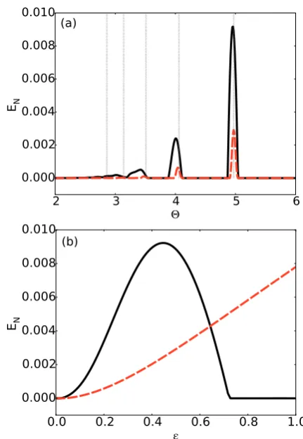
We see in Fig. 7(a) that very little entanglement is in fact generated in this system. For both forms of cou-pling there is no entanglement except, interestingly, for the values of Θ that correspond to trapping states which occur at integer values, n, such that sin(φ√n+ 1) = 0. Figure 7(b) shows how the entanglement at the n = 1 trapping state (Θ = 4.97 for N = 5) changes with the coupling strength ε, and we see that there is very dif-ferent behavior depending on how the micromasers are coupled. Indeed, the behavior is different again from that seen with either the relative phase or the mutual information: the logarithmic negativity grows quadrati-cally for both coherent and dissipative coupling, but the growth is most rapid for coherent coupling in contrast to both the relative phase and the mutual information. The logarithmic negativity eventually peaks and decays before vanishing around ε ∼ 0.7 for the case of coher-ent coupling. Very similar behavior was seen in another system of coupled nonlinear oscillators where trapping ef-fects restrict the state-space available to the system [45]. In that case vanishing of the entanglement for sufficiently strong coupling was found to be intimately linked to the restricted state-space and the same factors seem likely to be at work here. Overall, however, for both cases the

(a)

(b)

FIG. 7: (Color Online) Entanglement for the coherent (solid, black) and dissipative (dashed, red) couplings forN= 5. (a) Logarithmic negativity forε= 0.5 over a range of Θ =φN1/2_. The dotted lines indicate the locations of the trapping states (n = 1,2,3,4,5). (b) Logarithmic negativity as a function of the coupling strength varied around the trapping state at Θ = 4.97.

most important point is that the entanglement remains very weak, even in the strongly quantum regime of very low photon numbers.

VII. CONCLUSIONS AND DISCUSSION

We have investigated synchronization effects in cou-pled micromasers using the relative phase distribution as a tool to quantify the emergence of preferred rela-tive phases. We used perturbation theory to show that dissipative coupling between the micromasers leads to a 2π-periodic relative phase distribution whose peak grows linearly with the coupling. In contrast, for coherent cou-pling the phase distribution isπ-periodic and there is a quadratic dependence on the coupling.

steady-state distribution which depended on just the cou-pling strength and the linewidth of the uncoupled micro-maser. This derivation also showed quite clearly that the phase dynamics would be much more complicated in the quantum regime where photon occupation numbers are low. Indeed, comparisons of numerical calculations using the full master equation showed that the Fokker-Planck equation substantially underestimated the strength of the features which emerge in the relative phase distribution in the quantum regime. Interestingly, a very similar un-derestimate of synchronization effects was obtained using a semiclassical model for the case of two van der Pol os-cillators [7]. In our case, it seems that low photon occu-pation number is the key factor that leads to differences between quantum and semiclassical predictions.

We also investigated the behavior of the mutual in-formation and entanglement of coupled micromasers and found that the behavior was rather different to that of the relative phase distribution. This is perhaps not sur-prising as the relative phase distribution depends on a very specific combination of a sub-set of the elements of the full density matrix of the system. Whilst one might

expect all forms of correlation to increase with coupling, at least initially, there is no obvious reason why differ-ent measures of correlation between the oscillators should increase in precisely the same way as the relative phase distribution.

Our work could serve as a starting point for a number of future studies. For example, it would be interesting to explore synchronization in the bistable regime where the micromasers exist in a mixed state consisting of limit-cycles with two different amplitudes. Another possibility would be to explore synchronization effects in systems with more than two micromasers. The perturbation ap-proach that we used here could prove a useful tool in analysing systems with a handful of coupled oscillators where a numerical solution of the full master equation already becomes very challenging because of the poten-tially very large state space involved. Finally, it would be interesting to investigate in detail the range of couplings which could be achieved in practice with micromasers, as well as solid-state analogs, and the best way to measure features in their relative phase distribution.

[1] A. Pikovsky, M. Rosenblum, and J. Kurths, Synchroniza-tion: A Universal Concept in Nonlinear Sciences, Cam-bridge Nonlinear Science Series (CamCam-bridge University Press, Cambridge, UK, 2003).

[2] J. D. Cresser, W. H. Louisell, P. Meystre, W. Schleich and M. O. Scully, Phys. Rev. A25, 2214 (1982). [3] L. Fabiny, P. Colet, R. Roy and D. Lenstra, Phys. Rev.

A47, 4287 (1993).

[4] O.V. Zhirov and D.L. Shepelyansky Phys. Rev. Lett. 100 014101 (2008).

[5] A. Mari, A. Farace, N. Didier, V. Giovannetti and R. Fazio, Phys. Rev. Lett. 111, 103605 (2013).

[6] M. Ludwig and F. Marquardt Phys. Rev. Lett. 111, 073603 (2013).

[7] T. E. Lee and H. R. Sadeghpour, Phys. Rev. Lett.111, 234101 (2013).

[8] G. Manzano, F. Galve, G. L. Giorgi, E. Hernndez-Garcia, and R. Zambrini, Sci. Rep.3, 1439 (2013).

[9] S. Walter, A. Nunnenkamp and C. Bruder, Phys. Rev. Lett.112, 094102 (2014).

[10] T. E. Lee, C.-K. Chan and S. Wang, Phys. Rev. E 89, 022913 (2014).

[11] I. Hermoso de Mendoza, L. A. Pach´on, J. G´ omez-Garde˜nes, and D. Zueco Phys. Rev. E90, 052904 (2014). [12] S. Walter, A. Nunnenkamp and C. Bruder, Ann. Phys.

527, 131 (2015).

[13] M. Xu, D. A. Tieri, E. C. Fine, J. K. Thompson, and M. J. Holland Phys. Rev. Lett.113, 154101 (2014). [14] M. R. Hush, W. Li, S. Genway, I. Lesanovsky and A. D.

Armour, Phys. Rev. A91, 061401 (2015).

[15] V. Ameri, M. Eghbali-Arani, A. Mari, A. Farace, F. Kheirandish, V. Giovannetti and R. Fazio, Phys. Rev. A.91012301 (2015).

[16] B. Zhu, J. Schachenmayer, M. Xu, F. Herrera, J. G. Re-strepo, M. J. Holland and A. M. Rey, New J. Phys. 17,

083063 (2015).

[17] L. Morgan and H. Hinrichsen, J. Stat. Mech., P09009 (2015).

[18] T. Weiss, A. Kronwald and F. Marquardt, New J. Phys. 18, 013043 (2016).

[19] V. M. Bastidas, I. Omelchenko, A. Zakharova, E. Sch¨oll and T. Brandes, Phys. Rev. E92, 062924 (2015). [20] W. Li, C. Li and H. Song, Phys. Rev. E 93, 062221

(2016).

[21] T. Weiss, S. Walter and F. Marquardt, e-print arXiv:1608.03550.

[22] N. L¨orch, E. Amitai, A. Nunnenkamp and C. Bruder, Phys. Rev. Lett.117, 073601 (2016).

[23] H. Walther, B. T. H. Varcoe, B.-G. Englert and T. Becker, Rep. Prog. Phys.69, 1325 (2006).

[24] P. Filipowicz, J. Javanainen and P. Meystre, Phys. Rev. A34, 3077 (1986).

[25] B. G. Englert, e-print arXiv:quant-ph/0203052; B. G. Englert and G. Morigi, Lect. Not. Phys. f611, 55 (2002). [26] S. Rinner, E. Werner, T. Becker and H. Walther, Phys.

Rev. A74, 041802 (2006).

[27] M. O. Scully, H. Walther, G. S. Agarwal, T. Quang and W. Schleich, Phys. Rev. A44, 5992 (1991).

[28] T. Quang, G. S. Agarwal, J. Bergou, M. O. Scully, H. Walther, K. Vogel and W. P. Schleich, Phys. Rev. A48, 803 (1993).

[29] W. C. Schieve and R. R. McGowan, Phys. Rev. A48, 2315 (1993).

[30] R. R. McGowan and W. C. Schieve, Phys. Rev. A55, 3813 (1997).

[31] D. A. Rodrigues, J. Imbers, and A. D. Armour, Phys. Rev. Lett.98, 067204 (2007).

[32] M. Marthaler, J. Lepp¨akangas, and J. H. Cole, Phys. Rev. B83, 180505 (2011).

[34] D. G. Aronson, G. B. Ermentrout and N. Kopell, Physica D41, 403 (1990).

[35] A. Kuznetsov, N. Stankevich and L. Turukina, Physica D: Nonlinear Phenomena 238, 1203 (2009).

[36] C. C. Gerry and P. L. Knight, Introductory Quantum Optics, (Cambridge University Press, Cambridge, UK, 2004).

[37] D. T. Pegg and S. M. Barnett, Phys. Rev. A 39, 1665 (1989).

[38] U. Leonhardt, Measuring the Quantum State of Light

(Cambridge University Press, Cambridge, UK, 1997). [39] S. M. Barnett and D. T. Pegg, Phys. Rev. A 42, 6713

(1990).

[40] A. Luis and L. L. S´anchez-Soto, Phys. Rev. A 53 495

(1996).

[41] J. R. Johansson, P. D. Nation and F. Nori, Comp. Phys. Comm.183, 1760 (2012); J. R. Johansson, P. D. Nation, and F. Nori, Comp. Phys. Comm.184, 1234 (2013). [42] R. L. Stratonovich, Topics in the Theory of Random

Noise, Vol. II (Gordon Breach, New York, 1967). [43] For dissipative coupling the expansion is in terms of ˜ε

and the terms in Eq. 18 form the perturbation.

[44] G. Vidal and R.F. Werner, Phys. Rev. A 65, 032314 (2002).