Electron cyclotron heating and current drive using the electron Bernstein modes

(1)

Electron Cyclotron Heating and Current

Drive using the Electron Bernstein Modes

Duncan Ekundayo McGregor

Thesis submitted for the degree of Doctor of Philosophy

of the University of St Andrews

(2)

Declaration

I, Duncan E. McGregor, hereby certify that this thesis, which is approximately 20,000 words in length, has been written by me, that it is the record of work carried out by me and that it has not been submitted in any previous application for a higher degree.

Date: ... Signature of Candidate: ...

I was admitted as a research student in September 2002 and as a candidate for the degree of Doctor of Philosophy in September 2003; the higher study for which this is a record was carried out in the University of St Andrews between 2002 and 2006.

In submitting this thesis to the University of St Andrews I understand that I am giving permission for it to be made available for use in accordance with the regulations of the University Library for the time being in force, subject to any copyright vested in the work not being affected thereby. I also understand that the title and abstract will be published, and that a copy of the work may be made and supplied to any bona fide library or research worker, that my thesis will be electronically accessible for personal or research use, and that the library has the right to migrate my thesis into new electronic forms as required to ensure continued access to the thesis. I have obtained any third-party copyright permissions that may be required in order to allow such access and migration.

I hereby certify that the candidate has fulfilled the conditions of the Resolution and Regulations appropriate for the degree of Doctor of Philosophy in the University of St Andrews and that the candidate is qualified to submit this thesis in application for that degree.

(3)

Dedication

This thesis is dedicated to my parents Douglas and June McGregor, for their support and encouragement throughout my life.

Acknowledgements

This work has been funded jointly by the UK Engineering and Physical Sciences Re-search Council and by EURATOM.

Special thanks must go to my supervisor Alan Cairns, who has continued to support me, provide guidance and inspiration, and show limitless patience, throughout my PhD, and especially during my period of illness. This thesis has benefited more than I can say from his suggestions, and I could not have asked for a more supportive supervisor.

Chris Lashmore-Davies and Martin O’Brien have provided me with guidance, en-couragement, and ideas on all my visits to Culham, and all of my work has benefited from their helpful suggestions.

My office mates Gavin Donnelly and James McLaughlin have provided me with moral support, and countless stimulating conversations. The last few years would not have been as entertaining without them.

(4)

Abstract

Electron Bernstein waves are a mode of oscillation in a plasma, thought a candidate for providing radiofrequency heating and non-inductive current drive in spherical tokamaks. Previous studies of these modes have relied on neglecting or simplifying the contribution made by relativistic effects.

This work presents fully relativistic numerical results that show the mode’s dispersion relation for a wide range of parameters. Relativistic effects are shown to shift the location of the resonance as in previous studies, but the effects beyond this are shown to matter only in high temperature (10-20keV) plasmas. At these higher temperatures however, the fully relativistic model differs markedly. The as-sumption that the mode is electrostatic is looked at, and found to be inadequate for describing fully the electron bernstein modes dispersion relation.

Simple estimates that neglect toroidal effects show current drive efficiency is expected to be an order of magnitude higher than that for conventional electron cyclotron current drive using the O or X modes. It is shown for a number of model tokamaks that heating the center of the plasma and driving cur-rent using EBWs is impossible launching from the outside due to strong damping of the wave at higher cyclotron harmonics.

Results from a code based on a more complicated semi-analytic model of current drive, that in-cludes toroidal effects and calculates the average current drive over the magnetic surface, confirm the higher expected current drive efficiency, and the code is shown to give good agreement with a Fokker-Planck code. The higher values of

associated with the EBWs are shown to mitigate the delterious effects of trapping on current drive efficiency to a small extent. The details of the magnetic field are found to be unimportant to the calculation beyond determing where the wave is absorbed.

(5)

Introduction

1.1 FUSION

Because the most strongly bound nuclei are those of elements in the middle of the periodic table, it is possible to release nuclear energy by the fusion of lighter nuclei to form heavier ones. The most suitable reactions for obtaining this energy in a controlled manner are the fusion of isotopes of hydrogen to form helium. Of these reactions, that with the lowest activation energy is the fusion of an ion of deuterium and an ion of tritium to form helium and a neutron

! #"

(1.1)

Whilst successful fusion is still a goal, research is likely to focus on this reaction, but as tritium is an unstable radioactive gas it may eventually be desirable to switch to deuterium-deuterium fusion

$%

(1.2)

although this reaction has a higher activation energy.

The chief obstacle to obtaining this energy is the Coulomb repulsion between the positively charged atomic nuclei. For fusion to occur the reacting nuclei must have sufficient energy to over-come this force of repulsion. In the case of D-T fusion the reaction cross-section (the probability of the reaction taking place) is at its maximum when the particle energy is of the order &('

#"

Thus for fusion to yield large quantities of energy, the particle thermal energy must be of this order also. Thermal energy of&('

#"

is approximately equivalent to&)+*,

(9)

1.2 THE TOKAMAK

1.2.1 The Basic Tokamak

In order to contain the reactants, and obtain temperatures of sufficient magnitude for fusion to take place, several magnetic containment devices have been built. The device which currently looks most promising is the tokamak, illustrated in Fig 1.1.

Fig 1.1 A conceptual illustration of a tokamak [43]

The principal means of confinement is the toroidal magnetic field, generated by a series of current carrying external coils around the torus, but this field by itself will not confine the plasma. A charged particle travelling around the torus will orbit the magnetic field line it travels around, thus it will see a changing major radius and hence a changing magnetic field strength. This changing magnetic field strength will cause electrons and ions to seperate in the vertical plane so give rise to a vertical electric field and so there will be a gradual outwards drift in the particle’s path around the torus (the so-called

-/.10

drift). Thus it impossible to confine a plasma with just a toroidal field. Fortunately the problem can be solved by adding a small poloidal component to the magnetic field.

(10)

toroidal direction. In present day experiments the plasma current is driven by a toroidal electric field induced by transformer action in which a flux change through the torus is generated as illustrated in Fig 1.2. The flux change is brought about by a current passed around the primary coil around the torus as shown in Fig 1.3.

Fig 1.2 A change of flux through the torus induces a toroidal electric field which drives the toroidal current. [7]

Fig 1.3 A change of flux through the torus induces a toroidal electric field which drives the toroidal current. [7]

(11)

In the effort to overcome these limitations numerous refinements and alterations to the basic model of the tokamak have been attempted. For instance, it has been found that vertically elongating the plasma can be advantageous. This requires additional toroidal currents. One can also control the position of the plasma with such currents. Thus most working tokamaks contain further suitably placed coils to generate such currents - the complete system of toroidal and poloidal coils is illustrated in Fig 1.4.

Fig 1.4 Arrangement of coils in a tokamak [7]

Another suggestion has been the so-called spherical tokamak.

1.2.2 The Spherical Tokamak

The advantages of the spherical torus concept were first outlined by Peng and Strickler in 1986 [1], but the ideas behind it come from earlier studies into other containment devices, the tokamak obviously, but also the toroidal pinch [2], and the spheromak [3]. The fundamental idea was to reduce the centre column of the tokamak to as small a diameter as possible, thus reducing the major radius of the tokamak, and so increasing the efficiency of the magnetic confinement. The higher magnetic field strength at the edge of the plasma means one can confine a denser plasma than is the case in a typical tokamak.

(12)

Fig 1.5 MAST: The Mega-Amp Spherical Tokamak, operating in UKAEA Culham Division [44]

The central column plays an important role in a tokamak however, housing the ohmic column, the inboard poloidal field coils, and shielding against fusion neutrons. In a conventional tokamak it may also include further coils to control the shape and position of the plasma. Thus the disadvantage of the space constraints imposed by the spherical tokamak model can outweight the advantages, and at present conventional tokamaks are still thought the most likely candidate for successfully generating energy from nuclear fusion. There is also the second disadvantage that the plasma’s relative density and magnetic field strength are such as to hinder some methods of heating the plasma. In spite of these difficulties, the greater efficiency of magnetic confinement they are capable of delivering may make them a more desirable model for fusion power plants in the future.

1.3 RADIOFREQUENCY HEATING AND CURRENT DRIVE

The toroidal current in a tokamak also heats the plasma through ordinary resistive, or Ohmic, heating. Unfortunately, a plasma’s electrical resistivity decreases with temperature, as32

4!5 so as

tem-perature increases Ohmic heating becomes less effective. [7] This would mean that vast quantities of energy would be required to heat a plasma to the temperatures required via Ohmic heating, making it unattractive as a means of generating power. Also, the plasma’s stability is dependent on the toroidal current, so it may not be feasible to drive such large currents around the tokamak whilst containing the plasma. For these reasons, if the temperature is to be raised to the level required for nuclear fusion, some form of auxiliary heating is required.

(13)

electro-magnetic waves tuned to some natural resonant frequency of the plasma so as to be absorbed transferring their energy to the plasma particles. This requires that it be possible to launch a wave from an antenna or waveguide at the plasma edge, and that the wave be able to propagate to the central region of the plasma and be absorbed there.

Radiofrequency heating may have a secondary use in a fusion reactor, such as a tokamak, though - that of controlling the plasma profile. In Ohmic heating, the current and energy deposition profiles are determined by the transport properties of the plasma [7] making it difficult to control these profiles. Radiofrequency absorption, however, may be localised and its position controllable, particularly in the higher frequency ranges, allowing it to be used to alter the plasma temperature profile in such a way as to suppress instabilities.

A further application of radiofrequency waves is to current drive. The normal inductive method of current drive, by its very nature, leads to pulsed operation. The plasma current can only be maintained for as long as the magnetic flux linking the plasma torus is changing monotonically. This would create sig-nificant engineering problems in any potential fusion reactor, thus much research effort has been devoted to schemes for producing steady state current drive. One method by which this might be achieved uses radiofrequency waves to set up a drift of electron around the torus as they are absorbed by the plasma. There are several methods by which this can be done, and we will outline two of them in Section 1.6 where we talk about the particular methods of current drive we are investigating in more detail. It bears remarking upon the fact that our ability to control where the radiofrequency waves are absorbed can be exploited in current drive as well as in heating, this time to control the plasma’s current profile. Since some of the major magnetohydrodynamic instabilities depend on the plasma’s current profile [7], this is a very important application of wave current drive.

The schemes which have been investigated for radiofrequency heating of tokamaks can be divided into four frequency ranges. In increasing order of frequency, they are

(i) Alfven Wave Heating involving waves at a frequency of a few MHz

(ii) Ion Cyclotron Heating involving waves at a frequency of a few tens of MHz (iii) Lower Hybrid Heating involving waves at a frequency of a few GHz

(iv) Electron Cyclotron Heating involving waves at frequencies of around 30GHz and upwards.

It is the last of these methods that we are concerned with, and go on to speak about in the next section.

1.4 ELECTRON CYCLOTRON HEATING

1.4.1 Introduction

(14)

electron laser, capable of generating very high powers at frequencies in excess of 100GHz.

Because the high frequencies of wave being used makes tunneling impossible in all but the smallest of devices, ECRH requires that it be possible to launch a wave from an antenna or waveguide at the plasma edge, i.e. the wave must be capable of propagating in a vacuum and at the plasma edge. Whilst this limitation is not an advantage per se, the ability to propagate in a vacuum has desirable consequences. In other heating methods, the waves used are often evanescent in a vacuum, and require to tunnel through a region in which they are non-propagating to reach the plasma interior - a significant fraction of the incident power is thus reflected, and can result in a high amplitude standing wave at the plasma edge. They may also require complicated internal structures to assist the waves on reaching the plasma interior - such structures will inevitably deteriorate as a result of the temperature and particle bombardment, and can give rise to impurities in the plasma. These difficulties need not concern us in ECRH, which requires only simple waveguide launching.

Assuming the wave can be launched acceptably, it also requires to be capable of reaching the plasma interior, and being absorbed there. In considering the first condition, we may disregard thermal effects, but the absorption necessitates the inclusion of these effects. Thus we look first at the propagation of waves in general, then go on to consider the cold plasma dispersion relation, and lastly the hot plasma dispersion relation.

1.4.2 Propagation of Electromagnetic Waves in a Plasma

Propagation of electromagnetic waves in any physical medium is governed by the Maxwell Equa-tions

6 .7- 8 9;:

0

:=<

(1.3)

6

.?> 8 @

:=A :=<

(1.4)

6CB 0 8

&

(1.5)

6CB

A

8 D

(1.6)

where all quantities are functions of configuration space and time e.g. -E8E-GFIH

5

<J .

(i)

-is the electric field intensity in Volts per metre or Newtons per Coulomb. (ii)A is the electric displacement vector

(iii)0

is the magnetic induction in Tesla (iv)>

is the magnetic intensity (v)D

is the electrical charge density in Coulombs per cubic metre (vi)@

is the electrical current density in Amps per square metre. The relations between

-andA , and between

0

and>

are dependent on the particular physical medium. The plasma medium is remarkably varied in this respect, but provided all external electric fields are of moderate intensity, a plasma can be assumed to behave, for all intents and purposes, like an anisotropic dielectric medium. Thus we need only consider the linear response of the plasma to the fields, and may neglect nonlinear effects.

A

8LK B -L8EKMN B

(15)

where is a rank two tensor, the dielectric permitivity tensor. Similarly but we typically assumeP,8$PRM

wherePRM

is the permeability of free space.

Related to the permittivity is the conductivity S of the plasma defined such that @78 S B (1.8)

Defining the conductivity so, and assuming we are at liberty to Fourier transform in both time and space so the fields vary asTVU FXWZY B H[9?W]\

<J we may express the permittivity in terms of the conductivity

tensor

K[8EKM^_9 S`

W]\

(1.9)

which will be useful later in calculating the hot plasma dispersion relation. For now, taking the curl of (1.3)

6 .aF6

.?-J

8 9 : :=<

F 6 .?0

J

8 9bPRM : :c< F 6 .7> J 8 9bPRM : @ :=< 9aPRM : A :=< (1.10)

assuming no external current this becomes

6 .aF6

.?-J PRM+KM : :=<

FIN B

-J

8

&

(1.11)

To obtain the local dispersion relation we assume that the plasma is uniform and homogeneous in space and time thus we may Fourier transform these equations, or equivalently, assume that

- 8

+dXegfVhi 2kjlnm

(1.12)

0 8 0 M

0 dXegfVhi 2kjVlnm 5 (1.13)

and0 M

is the static magnetic field and is taken to be in the z-direction, and o

0 opqo 0 M o

Then, in terms of the plasma refractive index,r

8sfut

j

5 we obtain

r .vF r .7-J

N B -L8

&

(1.14)

where we have usedPRMKM8

`uw

We can write this in tensor form

x B -L8 & (1.15) where x 8 yz { *}|| 9 ~ *| *|+ ~ * | * 9 ~ 9 * * %| ~ * % * 9 (1.16)

Non trivial solutions exist for

<

x 8 &

Thus for values ofr ,

\

consistent with the local dispersion relation we must calculate the dielectric tensor elements then solve the linear problem

(16)

1.4.3 The Cold Plasma Dispersion Relation and Propagation of the O and X-Modes

There exist two wave modes, both capable of propagating in a vacuum, for which the cyclotron resonance and its harmonics are accessible. These modes are called the ordinary and extraordinary modes. We will outline where their cold plasma dispersion relations come from, and give an account of their properties that are relevant to electron cyclotron heating.

The dielectric tensor elements in the cold plasma approximation are calculated from the so-called ”two-fluid equations,” where the plasma is treated as two separate fluids, one of ions, one of electrons. Only electromagnetic forces are taken into account. We begin with the equations:

: :c< M 6CB+ 8 & (1.17) < 8 .?0G J (1.18)

Assuming these are suspectible to Fourier analysis we can can readily obtain an approximation for

in terms of-

From this we proceed to express in terms of

-5

and then using

8 S B -(1.19) N8^ S

W]\K M (1.20)

The method is well known, so we omit the specifics. After some simple analysis the cold plasma disper-sion relation is found to be

* || 9 ~ * | ~ * | * 9 ~ 9 & ~ & * 9 8 & (1.21) where *}|| 8 * 8 9 \ \ 9\ t 5 (1.22) * | 8C9 * |

8 9bW

\ \ t \F\ 9\ t J 5 (1.23) * 8 9 \ \ 5 (1.24) where\ 8F M ` KM J 4

is the plasma frequency of species and

\ t 8 o o M `

is the cy-clotron frequency for species

If now restrict ourselves to electron terms only (and henceforth omit the subscript ), since the frequencies being considered are far too high for the waves to have any interaction

with ions, this dispersion relation reduces to the well-known Appleton-Hartree dispersion relation for a wave propagating at an angle of to the steady magnetic field.

(17)

where is the plasma refractive index, « 8/F\ tª¤ ¥¦¨§ ¬ \ F 9 ¢J ®°¯ ¥ J 4 (1.26) and ¢ 8 \ ¤ \ (1.27) The

sign gives the ordinary mode (or O mode), and the 9

sign the extraordinary mode (or X mode). We will assume propagation to be perpendicular to the steady magnetic field so as to see most clearly the essential features of propagation.

The O mode’s dispersion relation simplifies to

8 9 \ \ (1.28)

which is simply understood. The wave will propagate until the density reaches the point where\

8\

Thus for the l¨±

cyclotron harmonic to be accessible to the wave, we require

\ }² \ tª¤ (1.29)

In a conventional tokamak, the plasma and electron cyclotron frequencies in the centre of the plasma are typically of the same order of magnitude, making this an important consideration in any electron cyclotron heating scheme. In a spherical tokamak the plasma frequency is generally higher, and typically the interior of the plasma is inaccessible to the O mode.

The X mode’s dispersion relation simplifies to

8 F\ 9\ J 9\ tª¤ \ \ F\ 9\ 9\ tZ¤ J (1.30)

which is less simple than the O mode. There exists a cut-off ( 8

& ) where F\ 9\ J J 8\ tª¤ \ (1.31)

and a resonance ( ´³

), the upper hybrid resonance, where

\ 8$\ ¤ \ tª¤ (1.32)

For non-perpendicular propagation, the O mode cut-off and the upper hybrid resonance are unaf-fected, but the condition for cut-off of the X mode is changed to

µ 9 \ ¤ \ 9\ tª¤ 9 ~¶ 9 µ \ ¤ \ tª¤ \F\ 9\ tª¤ J ¶ 8 & (1.33) which gives F\ F 9 ~ J 9\ ¤ J 8\ \ tª¤ F 9 ~ J (1.34)

We can see how these cut-offs and resonances affect propagation across an inhomogeneous mag-netic field by constructing a Clemmow-Mullaly-Allis (CMA) diagram, (Fig 1.6), plotting these cut-offs and resonances in terms of·

8\ ¤ ` \ , ¸ 8\ tª¤ ` \

(18)

Fig 1.6 CMA diagram for the X mode. The wave does not propagate in the shaded region or in the region to the right of all the curves.

The X mode does not propagate in the shaded region - thus saving the case of a very small machine where evanescent tunnelling might still be possible, accessibility for the X mode requires that the path traced out on this diagram as the wave propagates from the plasma edge to the desired resonance not cross this region. At the edge of the plasma·

8

&

, since the density goes to zero, thus we always begin at the

¸ -axis. The magnetic field strength increases as we move towards the center of the tokamak, thus if we

launch our wave from the outside the path will go upwards, whereas launching the wave from the inside, the path will go downwards. At the fundamental cyclotron resonance, Y=1, thus this is only accessible from the high field side. There is also the density limit to be considered, since the wave must reach the cyclotron resonance before it encounters the high density cut-off. If we consider the case ~

8

&

gives the condition·;`¹¸

²

¡ , i.e.

\

¤

\

tª¤

²

¡ (1.35)

The other commonly used scheme is the second harmonic, corresponding to ¸

8

This is accessible from both the outside and the inside. From the outside requires the resonance be reached before the left hand branch of the cut-off, giving the condition·

²

when\8

¡

\

tZ¤, i.e.

\

¤

²

\

¡

8

¡

\

tª¤

(1.36)

From the inside we require·

²

when\8

¡

\

tZ¤ so that

\

¤ ²»º

¡

\

8

\

tZ¤

(1.37)

Launching the X-mode from the inside has the advantage that at both the fundamental and second har-monic it can reach higher densities than the O mode, which has the same density limit regardless of the direction of propagation. On the other hand, inside launch is technically less convenient. For a given magnetic field, the density limit is raised if one goes to the second harmonic, or a higher harmonic, but once again this is technically less convenient, as one will require a higher frequency source. We remark in passing that spherical tokamak’s relative density and magnetic field strength will often prevent the use of the X modes to heat the interior of the plasma also.

At non-zero'

~

(19)

in the plasma and for mode conversion to take place from one to the other ([11], [12]). This would allow us to launch an O mode from the edge of the plasma to the interior, then convert to an X mode, which will be absorbed at the upper hybrid resonance. The mechanism, due to Preinhalter and Kopecky [11], is as follows. The cut-off condition for the O mode,\

8¼\

¤

5

and X mode 1.34 are satisfied at the same point in the plasma if

F

9

~

J

F

\

tª¤ `

\

¤

J

8

(1.38)

when\

8\

¤

The wave dispersion relation is then as illustrated in Fig 1.7.

Fig 1.7 O and X mode dispersion curves for the value of parallel refractive index at which mode conversion between the two modes is possible

A wave incident in the O mode is partially reflected in the X mode, which, having its group and phase velocities in the opposite directions near the cut-off, continues to propagate in the same direction as the incident wave, but with its phase velocity in the opposite direction. When the density increases to the value at which\

`

\

¤ is equal to the value at the minimum on the X mode branch in Fig 1.7, the

group velocity reverses, and the wave travels back towards the low density region eventually reaching the position of the upper hybrid resonance. The existence of an additional set of modes around the cyclotron harmonics, the Electron Bernstein Waves, complicates matters, and the wave can convert into this mode before being absorbed.

1.4.4 The Hot Plasma Dispersion Relation

The hot plasma dispersion relation is derived from a kinetic description of the plasma where we treat it via a distribution function½

FIH

5

<%J , s labelling the particle species,

H

the position in configuration space,

the position in velocity space and t the time. The plasma’s behaviour is then described by the Vlasov Equation

: ½

:c<

,B :

:

H

½

¾

.?0

J

B :

:

½

8

&

(1.39)

where

is the charge of the species

5

the mass of particle species

5

-the electric field strength, and0

the magnetic induction.

We again assume that we may Fourier transform in space and time but this time take \

(20)

a small positive imaginary part when it becomes necessary to resolve the singularity in the momentum integrals and guarantee convergence. This was shown by Landau to be equivalent to treating the problem an an initial value problem, performing a Laplace transform in the variable'

, then deforming the contour of integration [10]. We also neglect the subscript

5

taking the terms to apply to electrons. We can then write (1.39) as

: ½ :=<

7B6

½

À¿

-Á

.ÂFI0GM

0

JZÃ Bu6GÄ

½

8

&

(1.40)

For a local dispersion relation we may assume we can Fourier Transform in time and configuration space; in resolving the singularity in the momentum integrals we take \

to to have a small positive imaginary part.

We take the usual co-ordinate system, with 0GM(F]Å

J

8

M°ÆVÇ

and choose '

8

' |

F

'

8

&

J and

use cylindrical co-ordinates in momentum space such thatÈ |ÊÉ

È

°¯ ¥ÌË

5

È

ÍÉ

È

¥¦¨§bË

We assume the field strengths to be small, allowing us to perform a perturbation expansion. We then write the first order distribution function in terms of another function

½

FIH

5

<%J

É

dXeÎf(hi 2kjVlnm

½

M F È J%Ï

F

J

(1.41)

Some analysis follows, and we eventually obtain an expression for the first order distribution funnction½

, from which we can calculate the plasma current

Ð

FIY

5

\

J

8 Ñ

ÑÒ

½

Ñ

FIY

5

\

J

U

(1.42)

and from the current we can obtain the dielectric tensor, from (1.8) and (1.9) which can be substituted into (1.14) and we can discover the modes present in a hot plasma.

(21)

Fig 1.8 Wave modes propagating perpendicular to a magnetic field. The broken line shows the cold plasma extraordinary mode, and the complete line the electron Bernstein modes.

The Electron Bernstein Modes are strongly absorbed at the electron cyclotron frequency and its harmonics, making them suitable for electron cyclotron heating.

We will not discuss in detail the mathematics of the hot plasma dispersion relation, as we look at it in detail in Chapter 2. For the moment we will mention only the resonance condition. Consider radiation near the l¨±

harmonic of the cyclotron frequency, then damping occurs in the non-relativistic theory as the result of the imaginary part in resonant integrals of the form

Ò Ó

F

È J \Â9

'

~

È

~

9 \ tª¤

È (1.43)

or, in physical terms, as a resonance between the wave and those particles whose parallel velocity is such that the Doppler shifted wave frequency which they see is a multiple of the cyclotron frequency. If we include relativistic mass dependence though, and let\

tª¤

M

be the electron cyclotron frequency calculated using the electon rest mass, the resonance conditions becomes instead

\Â9

'

~

È

~

9 \ tª¤

M

µ

9EÈ

w

¶

4

8

&

(1.44)

At lower temperatures this can simplified by Taylor expanding the last term and keeping the only the first two terms, giving

\Â9

'

~

È

~

9 \ tZ¤

M

µ

9

¡

È

w

¶

8

&

(1.45)

An approximate indication of the importance of the relativistic effect can be given by comparing the Doppler and relativistic frequency shifts in (1.45). If they are approximately equal, for typical particle velocities, then

'

~

È

~ Ô

¡

\

t

È

l¨±

w

Ô

¡

\

È

l¨±

w

(22)

or

~ Ô

È

l¨±

w

ÔÖÕ

¤

F

'

u"

J

!&& ×

4

(1.47)

For temperatures of a few keV it can be seen that (1.47) implies relativistic effects will have a significant bearing on results over a sizeable cone of angles around the perpendicular direction. This simple argu-ment is not intended to be a rigorous stateargu-ment of where relativistic effects are important, but merely to demonstrate the importance of relativity to the hot plasma dispersion relation at lower temperatures than might be expected.

1.5 ELECTRON CYCLOTRON CURRENT DRIVE

1.5.1 Introduction

Driving current around a tokamak is the second way in which it is envisaged that radiofrequency waves could be applied. Conventional current drive relies on inducing an electromotive force around the toroidal plasma by altering the magnetic flux passing through the centre. However, it is impossible that the magnetic flux change monotonically indefinitely, making the process pulsed in nature, though in a reactor the loop voltage is quite small (Ø

"

), and the pulses could be quite long, perhaps of the order of an hour. From the engineering point of view it would be much more convenient to have a reactor that could operate continuously, motivating research into non-inductive current drive. Even if this is not practicable, radiofrequnecy current drive might still have a role in suppresing magnetohydrodynamic instabilities by modifying the current profile, taking advantage of the localised absorption or radiofre-quency waves to generate current locally.

The essential feature of using radiofrequency waves for current drive is that they be absorbed in such a way as to produce some kind of asymmetry with respect to the toroidal direction. In electron cyclotron current drive, the resonant particles are mainly accelerated perpendicular to the magnetic field - this might at first glance appear to be of no value to producing current in the toroidal direction - but it was shown by Fisch and Boozer to be a perfectly viable method of driving current. We discuss how this occurs in Section 1.5.4.

There are several figures of merit used to characterise current drive efficiency. The thinking be-hind all of them is the desire that the maximum amount of current be driven for the wave energy put into the plasma. In theory, the efficiency is often the current density per unit absorbed power density. In ex-periment it is more often the total current driven per unit absorbed power. Both of these figures of merit are largely dependent on the temperature, particle density, and other plasma parameters that are charac-teristic of the tokamak rather than the method of current drive. This has prompted a new dimensionless

figure of merit ÙVÚ

É

K

M

¤

¤_Û+Ü ~Ý ¡!Þß

5

¿14Ã (1.48)

whereKM

is the permittivity of free space, ¤ and

¤ are respectively the local electron density and

ß

8áà

Ò

«âÍãåäæ

F

½ç Jè

(23)

is the absorbed power density (â is the particle energy). ãéä%æ is a quasilinear diffusion operator and ½ç

a Maxwellian distribution function.

Obviously, there is no one correct figure of merit to use, and we have varied in which we use as is appropriate to the problem considered, particularly when comparing our results with others’ who have used a particular figure of merit. Assuming the correct parameters are known, one can convert between two of these figures of current drive efficiency with relative ease.

The usual method of calculating current drive efficiency is to consider the electron distribution function for an electron distribution in which the effect of collisions is balanced by that of the wave, so that the distribution function will satisfy

: ½ :c<

8 : ½ :=< tªêëë : ½ :=<íìåî Ä ¤ (1.50)

The first term on the right hand side is a collision operator, most usually of the standard Fokker-Planck form, and the second is most commonly a quasi-linear diffusion term as detailed in Section 1.4.6. The

In the next section we will give a very brief outline of quasilinear theory, essential to our methods calculating current drive efficiency, then in the two sections following we will consider two methods of estimating the current drive efficiency, the Langevin Equations, and Adjoint Methods, then in section 1.5.5 we will consider the two methods of Electron Cyclotron Current Drive due to Fisch and Ohkawa.

1.5.2 Quasilinear Diffusion

Quasilinear theory was originally developed to deal with weak turbulence in non-equilibrium plas-mas. It deals with waves’ ability to react back on the equilibrium distribution function, and alter it so as to stabilize the equilibrium. The essential idea is to split the particle distribution function into a slowly varying average part, and a rapidly fluctuating part produced by the wave.

½ FIH 5 5 <J 8 ½ MF 5 <J ½ FIH 5 5 <%J (1.51) where ½ M

is a spatially averaged distribution function varying over a much longer time scale than the wave period on which ½

varies. Substituting this into the Vlasov equation, we then average each side, and obtain an equation for time evolution of½

M

in terms of½

We consider½

to evolve according to the usual linear theory, and obtain an expression for½

in terms of½

M

This expression is substituted into our equation for the time evolution of½

M

giving an equation of the form

: ½ M :c< 8 : : È d°ï d Ñ : ½ M : È Ñ (1.52)

where the coefficient

ï d Ñ theW Ü l¨±

entry of the quasilinear diffusion tensor. The derivation of

ï

for a magnetised plasma was undertaken by Kennel and Engelmann [?], and we will not repeat it here. The tensor is a complicated term, and reproducing the exact expression here would be unilluminating. The diffusion coefficient in the direction perpendicular to the steady magnetic field, the part of concern to the problem of ECRH and ECCD, can be written more simply as

ï 8 Þ ¡ ' ~¹ð ñ oòÊó Ð ñ 2 ò 2 Ð ñ ó F ð ~ ` ð J ò Ð ñ o

(24)

whereò ó ò

|

ò

is the right-hand circularly polarised electric field, andò

2

ò

|

ò

is the left-hand circularly polarised electric field.

This expression has been found to describe the evolution of the zero order distribution function quite accurately. Indeed it remains an adequate description of the distribution function for remarkably high wave amplitudes given the theory neglects non-linear effects in the evolution of the waves them-selves.

1.5.3 Langevin Equations

Our plasma can be represented adequately by a distribution function obeying the Fokker-Planck equation. This equation gives the distribution function relaxing to its thermal equilibrium Maxwellian form under the action of small angle collisions. The equation contains first order derivatives, which can be interpreted as friction forces, and terms with second order derivatives which are diffusion terms. The Maxwellian arises from the balance of these two terms.

There is however, an alernative way of describing a system of this type - the Langevin Equa-tions [17]. These are simply the equaEqua-tions of motion of individual particles under random forces whose statistical properties reproduce the same diffusion and friction as in the Fokker-Planck Equation. If the Fokker-Planck Equation is of the form

: ½ :c<

8

x B : ½

:

¡

A

B

:

½

:

(1.54)

then x

is the friction term and A is the diffusion tensor (a second order tensor). The corresponding

Langevin Equations are

< 8EôõF

<%J (1.55)

whereô

is a random force with the statistical properties

²

ôEö÷8ø9

x

(1.56)

and

²

ôõF <%J

ôÊF <ùnJ

ö÷8 ¡!A?ú

F

<

9

<íùûJ

(1.57)

This might not seem to be much of saving, as properly we would need to integrate over a large number of particle orbits with different forces randomly distributed in the correct way. However it was pointed out by Fisch and Boozer [18] that for high velocity electrons the diffusion terms are small compared to the friction terms, making it unecessary to consider a statistical ensemble of different forces to reproduce the correct behaviour - only the average slowing down need be calculated. We reproduce their argument below

We assume azimuthal symmetry around the magnetic field direction, so the electron distribution function depends on two variables, which for convenience we take to beÈ , the total velocity, and

ð

, the velocity component along the magnetic field, both normalised to the thermal velocity. The frictional terms in the high velocity limit of the Fokker-Planck equation are reproduced by the Langevin equations

(È <

8 9Lü

È

È (1.58)

ð

<

8 9ÊF

¡

þý

J

ü

È

(25)

where Z is the ion charge number, andü is the usual collision frequency for a thermal particle given by ü 8 Rÿ § ¬ Þ K M È l¨± (1.60)

We can now use (1.58) and (1.59) to calculate the increment in current produced by a wave which changed the initial values ofð and

È

This increment is calculated over the whole history of the particle which eventually ends up with zero velocity. Clearly this does not correpond to the physical reality, and should be thought of as the incorporation of the particle into the bulk of the Maxwellian distribution where collisional diffusion once again becomes important. One would expect the approximation to be good if the initial velocity is well above thermal. Since fast particles, by definition, carry current more effectively, the method has considerable utility.

To solve the equations, note that

ð (È 8/F ¡ þý J ð È (1.61)

so that ifð

M

5

È

M

denote the initial values

ð ð M 8 Õ È È M × ó (1.62)

The time integrated current carried by the particle is

Ò M Ü < 8 #È l¨± Ò M ð < 8 #È l¨± Ò M ð ð `u < ð (1.63)

Using (1.59) and eliminatingÈ through (1.62) this becomes

uÈ l¨± ü F ¡ ý J Ò M È M Õ ð ð M × 4 e ó m ð 8 uÈ l¨± ü F ¡ ý J È M ð M (1.64)

Then, thinking of a continuous process of pushing electrons at F

ð

5

È J to

F ð ú ð 5 È

ú È J

5

the ratio of current density to power density is

Ð 8 ü F b ý J È l¨± ú F È ð J ú F È J (1.65)

Note we have dropped the subscripts 0. The above holds for electrons interacting with the wave at some isolated point in velocity space. For a wave-particle interaction described in terms of the rate of change of distribution function produced we have

Ð

8 ¡

ü F ý J È l¨± È ð æ l ìåî Ä ¤ È È æ l ìåî Ä ¤ È (1.66)

(26)

1.5.4 Adjoint Methods

An alternative approach is the use of adjoint techniques [19], [20]. To illustrate the method, consider the steady state problem

: ½ :=< tªêëë : ½ :=< ìéî Ä ¤ 8 & (1.67) with : ½ :=< tZêíëë 8 ü Õ È : ½ : È ý ¡ È : : P F 9ÂP J : ½ : P × 8 ü3½ (1.68) whereP$8 È ~

`#È and again we take velocities to be normalised to the thermal velocity. This collision

term is the high velocity limit of the Fokker-Planck Equation. Whilst it lacks many of the properties of the exact collision operator (e.g. energy and momentum conservation) it is reasonable description of the particles in a high velocity tail, and provides an analytically tractable example.

We define the scalar product of two functions in velocity space to be

¿½ 5 Ã 8 Ò M È (È Ò 2 P ½ (1.69)

then with C, the operator defined in (4.15) we have

¿õ½ 5 Ã 8 ¿ =5

ù¨½ Ã (1.70)

where C’ is the adjoint collision operator given by

ù 8ø9 È : : È F È J ý ¡ È : : P Õ F 9ÂP J : : P × (1.71)

We now use (1.69)-(1.71) to calculate the response functions giving the current driven and the power absorbed for a given F

: ½R` :=<J ìåî Ä ¤

If we take

8

È

P

then we have

Íù 8ø9ÊF þý J P (1.72)

and from (4.9) and (4.15)

(27)

The power dissipated by collisions is

8 9

È

l¨±

Ò

¡

È

Õ

: ½ :c<

×

tZêíëë

È (1.75)

8

È

l¨±

Ò

¡

È

Õ

: ½ :c<

×

ìéî

Ä

¤

È

(1.76)

and we can combine these to obtain the current drive efficiency. The result is identical to that obtained by the Langevin Equations.

This technique has the advantage that it can be generalised to toroidal geometry. The example above illustrates the essential mathematics of adjoint techniques whilst avoiding involving us yet in the neoclassical transport theory necessary to generalise this technique to toroidal geometry.

1.5.5 Methods of Electron Cyclotron Current Drive

The electrons which are driven by an electron cyclotron wave are determined by the cyclotron resonance condition

\Â9

'

~

È

~

9 \

t

8

&

(1.77)

so that at different points in the absorption profile the change in \

t due to the magnetic field gradient

produces excitation at different values ofÈ

~

At a cyclotron resonance, particles are accelerated predominantly in the direction perpendicular to the steady magnetic field. This at first might not seem to useful in producing toroidal current, however, one needs to remember that increasing the velocity of a particle in any direction will decrease its colli-sionality. Thus if we preferentially heat particles travelling one one direction around the torus (which we will due to the cyclotron resonance condition) the electrons will collide with ions less often, and so we get a net transfer of momentum between the electrons and ions. The electrons will have a drift velocity in the direction that is preferentially heated, and the ions in the opposite direction. Thus we set up a torioidal current.

Of course, heating the electrons will also induce a relativistic mass shift, with a resultant decrease in the parallel velocity of the heated particles, which would act against the effect of reduced collisional-ity. However it has been shown the reduced collisionality has a greater effect.

There is the additional consideration, which will lead us onto the second method of electron cy-clotron current drive, of particle trapping. Because the strength of the magnetic field varies from the inside to the outside of the tokamak, an electron traveling around the tokamak will see different mag-netic field strengths as it circulates. The quantity P8

È

`u is an adiabatic invariant, and the total

particle energy

8

È

` ¡ must obviously be conserved also. Therefore as an electron passes from an

(28)

Fig 1.9 Region of velocity space where particles become trapped.

When one increases the perpendicular velocity of the electrons using ECRH, one pushes electrons into the loss cone as shown in Fig 1.9. These electrons make a net contribution of zero to the current driven (considering only this particular method of current drive - we should remark that the trapped particles do contribute to the bootstrap current) and this should also be taken account of in calculating the current drive efficiency of Fisch’s method.

Particle trapping need not be only a problem to electron cyclotron current drive however. Ohakwa suggested that one could use particle trapping, of itself, to drive a current, since if electrons travelling in one direction are trapped, there will be a net movement of electrons in the opposite direction, and hence we will drive a current around the tokamak in the opposite sense to the velocity of the particles we are heating.

1.6 WORK

(29)

(30)

Chapter 2

Propagation of the Electron Bernstein

Modes

2.1 INTRODUCTION

Electron cyclotron heating and current drive are produced in a conventional tokamak using the O and X modes. In a spherical tokamak such as MAST [5] though, the electron cyclotron frequency is lower in relation to the plasma frequency than in a conventional tokamak, with the consequence that the O and X modes at frequencies around the first or second harmonic have cut-offs near the edge of the plasma and so cannot propagate more than a few centimetres beyond the plasma edge. An alternative means of providing electron cyclotron heating and current drive is to make use of the Bernstein modes, which do not have a high density cut-off, and possess strong cyclotron absorption near harmonics of the electron cyclotron frequency.

The Bernstein mode has the disadvantage (from the theoretical point of view) that the wave’s per-pendicular wavelength can become comparable to the Larmor radius, making the usual assumption of small Lamor radius invalid. Our analysis must therefore be valid for arbitrary Larmor radius. The Bern-stein modes were previously analysed in this manner for weakly relativistic parameters [24], [25], but at higher temperatures it is likely electron with velocities comparable to c will contribute significantly to cyclotron heating and current drive necessitating a fully relativistic approach.

(31)

2.2 TRUBNIKOV’S EXPRESSION FOR THE DIELECTRIC TENSOR

Propagation of electromagnetic waves in any physical medium is governed by the Maxwell Equa-tions, which give us the electromagnetic wave equation, including the dielectric tensor, as described in Chapter One. In a hot plasma we require to calculate the dielectric tensor via the Vlasov Equation rather than fluid equations.

: ½ :=< 7B#6 ½ À¿ -¾

.vFI0 M

0 JZÃ B6 ½ 8 & (2.1)

We have taken as the variable in½

instead of

For a local dispersion relation we may assume we can Fourier Transform in time and configuration space,; in resolving the singularity in the momentum integrals we take \

to to have a small positive imaginary part, as explained in Chapter 1.

We take the usual co-ordinate system, with0GM(F]Å

J

8

M°ÆÇ

and choose'

8 ' | F ' 8 &

J and use

cylindrical co-ordinates in momentum space such thatU |GÉ U °¯ ¥=Ë 5 U GÉ U ¥¦¨§bË

We then write the first order distribution function in terms of another function

½ FIH 5 5 <%J É dXegfVhi 2kjVlnm ½ MFU J%Ï F J (2.2)

so that with 8

, the first order Vlasov Equation becomes

9bW]\ ½ ¾ WF ' ~ U ~ ' U °¯ ¥åË J ½ ¿ -Á . 0

Ã 6 ½ M F . 0GM J B6 ½ 8 & (2.3) sinceF .?0GM J B#6 ½ M8 &

Now observe that

6 ½ Mb8 9 ½ M (2.4) so F .70 J B6 ½ Mb8 & 5 (2.5) and 6 ½ 8 9 w K ½ ¾ ½ Ï 6 Ï (2.6) so F .70 M J Bu6 ½ 8 9K\ t ½ M deÎf(hi

2kjVlnm :åÏ : Ë 5 (2.7) whereK8 F J 5 and Bu6 ½ MÀ8 9 ½ M - B (2.8)

Subsituting (2.7) - (2.8) into (2.3) we may write, using cylindrical co-ordinates,

W Õ Ì\ K\ t 9 ' ~ U ~ ' U

w! Ë

K%\ t × Ï :éÏ : Ë 8 9 B - M (2.9)

This is a first order differential equation whose solution may be written as

(32)

with ` t ' ~ ~ ` t , 2 ' `

t , and

J , É ~ ò ò | °¯ ¥ 0 ò ¥¦¨§ 0 J

We may now letË

Mu9Lö¼9

³

and be guaranteed of convergence because of our earlier assumption that\

has a small positive imaginary part. By a change of variables, 0

8

Ë

93

this result may be rewritten Ï F J 8 M Ò M54!687 W:93 9ÂW 2!¿ ¥¦¨§ F)3 9 Ë J W Ë Ã F B -J " 2<; 3 (2.11)

The current is then given by

Ð FIY 5 \ J 8 Ñ ÑÒ ½ Ñ FIY 5 \ J U (2.12)

The current is related to the electric field strength through the conductivity tensorS @,8

S

B

-(2.13)

which is related to the dielectric tensor through the relation

N8>= S Wª\K M (2.14)

Thus we can derive the elements of the dielectric tensor from (2.12). The equation is still analytically tractable - there are two possible routes one can take. One can integrate over the phase3

first, leaving the 3d integral over momentum space to be performed numerically or through some simplifying assumption, or one can integrate over momentum first, leaving the phase integral to be performed numerically. We have opted for the latter. The resulting expression is wellknown, although the analysis needed to arrive at this expression, originally performed by Trubnikov does not appear to be as wellknown, so the derivation is given here.

Omitting constant factors the expression for the conductivity tensor is

S d Ñ 8 Ò Ò? M 3 ½ M(F J 4!687 FXW:93 9W 2 F ¥¦n§ F)3 9 Ë J ¥¦¨§bË J%J U d U ù Ñ

We takeU

in units of w so 78A@ U In Cartesians,

8 FU

°¯ ¥ÌË 5 U ¥¦n§bË 5 UB+B J ù

8 FU

°¯ ¥ F Ë 9C3 J 5 U ¥¦¨§ F Ë 9C3 J 5 UB+B J

If we now introduce

8 9bWõ: :ED dGFHI FKJ M ù 8 9bW: :ED ù dGFMLNHIL F L J M

the angular part of the integral is then

(33)

where the integral is over the the whole spherical solid angle.

The exponent is

W ÕTS =\ \ t × with ß | 8 ã | ã ù | °¯ ¥ 3Í9 ã ù ¥¦¨§ 3Í9 \ U \ t ¥¦¨§ 3 ß 8 ã ã ù | ¥¦¨§ 3 ã ù °¯ ¥ 3÷9 \ U \ t F 9 °¯ ¥ 3 J ß 8 ã ã ù

9 B+B3

\

U

\

t

where we have used

ù 8/FU | °¯ ¥ 3 U ¥¦¨§ 3 5 U °¯ ¥ 3Í9 U | ¥¦n§ 3 5 UB+B J

to remove terms involving

ù

We now perform the angular integration by taking the V

Å

V axis along the direction of

S

and letting

¢ be the angle between

S

and . The integral then becomes (just a standard spherical polar integral,

independent of the azimuthal angle)

Ò dGWXHI R 8 ¡!Þ ÒY M d[Z <\^] &`_

¥¦n§ ¢ ¢

8 ¬ Þ ¥¦¨§ F ß U J ß U

Now, the conductivity tensor is obtained from (dropping the¬ ÞJ 9 : : ã d : ã L Ñ Ò M 3 Ò M U 4!687 Fí9bPa WbÌ\ U \ t 3 J ¥¦¨§ F ß U J ß U

We now use the fact that

U 4!687 Fí9bPa WbÌ\ U \ t J 8/Fí9bP W \ U \ t J U 4!67 Fí9bPa W^=\ U \ t J

and integrate by parts to get (for theU

integral) Fí9bP W j c jKd 3 J Ò M U 4!687 Fí9bPa Wb=\ U \ t 3 J °¯ ¥ F ß U J

From the Bornatici et al review article [26] we obtain the relations

(34)

with * F 5 Å J 8 * . F]Å J Å .

So, the integral overU

gives * y { 5`i Õ P 9aW \ U \ t × ß

Since the vectorsã

5

ã

ù only appear in

ß we have

: * µ 5`j P 9ÂW j c jKd 3 ß ¶ : ãåd : ã L Ñ 8 : : ã L Ñlkm 9 * y { ¡ 5 i Õ P 9ÂW \ U \ t 3 × ß ¡ :éß : ãådTno 8 9 ¡ : ß : ã d : ã L Ñ * y { ¡ 5 i Õ P 9W \ U \ t 3 × ß ¬ :åß : ãåd :åß : ã L Ñ * y { º 5 i Õ P 9ÂW \ U \ t 3 × ß

The analysis from this point onwards is detailed and time-consuming, but the techniques are straightfor-ward and the details are omitted. Performing this analysis, one arrives at Trubnikov’s expression

N8^ Ñ Wª\ Ñ K Ñ \£\ t Ñ P * FXP J Ò M 3Pp * Frq s J s t 9 * Frq s J s 4 tvuw (2.15) where sL8/FXP?9ÂW^3 \ K Ñ \ t Ñ J ¡ ü F 9 °¯ ¥ 3 J ü ~ 3 (2.16) whereü ~ 8 ~ \ ` K Ñ \ t Ñ ,ü 8 \ ` K Ñ \ t Ñ , and t 8 yz { °¯ ¥ 3 9 ¥¦¨§ 3 & ¥¦¨§ 3 °¯ ¥ 3 & & & (2.17) and t u 8 yz { ü ¥¦¨§ 3 9 ü ¥¦¨§ 3cF 9 °¯ ¥ 3 J ü ü ~ 3 ¥¦¨§ 3 ü ¥¦¨§ 3cF 9 °¯ ¥ 3 J 9 ü F 9 °¯ ¥ 3 J ü ü ~ 3cF 9 °¯ ¥ 3 J ü ü ~ 3 ¥¦¨§ 3 9 ü ü ~ 3cF 9 wx 3 J ü ~ 3 (2.18) and*

. is the modified Bessel Function of the Second Kind (or McDonald Function), of order

Alter-natively, one can integrate over3

(35)

2.3 EVALUATION OF THE DIELECTRIC TENSOR

Previous work on the dielectric tensor has involved making further analytic progress by such assumptions as F

È`uw J p

, making a non-relativistic, or a weakly relativistic, approximation possible. We have opted instead to use numerical integration immediately, thus evaluating the fully relativistic dielectric tensor, in the belief that the complete relativistic correction may prove relevant in a functional tokamak. Certainly for temperatures less than 5keV such effects are negligible, but at the temperatures of around 10-20keV that one might reasonably expect in a working power plant, such effects could prove significant.

The task of evaluating the dielectric tensor is more difficult than one might expect though. If we look at the integrand we are required to evaluate, Fig (2.3.1)-(2.3.2),we can see immediately the integrand is oscillatory, and moreover slowly convergent, making evaluation a difficult, not to say time-consuming, process. Fortunately, the integrand is loosely periodic as is illustrated when we plot it with the function

°¯

¥ . We have plotted these functions against

3

(36)

Figure 2.3.1: The real part of the integrand plotted alongside cos(s) for &

5

~

&

º

5

' #"

5

\

`

\

8

¹

Figure 2.3.2: The imaginary part of the integrand plotted alongside cos(s) for

8

&

5

~

8

&

º

5

8

' #"

5

\

`

\

8

(37)

Thus it is considerably easier to evaluate ÿ ¦Gy .z F [ ã|{ J (2.19) where ã { 8 { Ñ J W]\ K Ñ \£\ t P * FXP J Ò Ñ Y 4 e Ñ 2 m Y 4 3 p * Frq s J s t 9 * Frq s J s 4

t u w (2.20)

Though evaluation of this integral can still be time-consuming, the calculation is considerably quicker, and easier.

Our program calculates this sum, stopping when it considers the integral to have converged, the convergence condition we set beingã {

9 ã { 2 ² . &¹2

. Though greater precision could be asked

for, this accuracy is close to the square root of machine precision, generally accepted as the smallest precision worth asking for.

Each integral is evaluated using Romberg’s Method, which uses k successive refinements of the extended trapezoid rule

Ò |} |~ ½ FT J T ¿ ¡ ½ ½ $ûûu ½ { 2 ¡ ½ { Ã (2.21) where T 5 T 5 ûû 5 T

{ is an equally spaced partition of the interval

¿ T 5 T { Ã, 8 T 9 T 2 , and ½ 8 ½ F T J

By refinement, we mean doubling N, so the interval is split into a greater number of points, closer together. We then treat the integral as a function of h, and extrapolate the continuum limit

8

&

, from our k existing results.

By taking the integral in manageable intervals ofÞ ` ¡ we ensure we are only required to integrate

a smooth analytic function, a task which Romberg’s method is well suited to. We have also experimented with methods using variable step sizes, but such methods have proved slower, and less reliable.

In Figs (2.3.3)-(2.3.4) we show the behaviour of the top left element of the dielectric tensor over a range of\

t

`

\

which includes the first few cyclotron harmonics. This figure shows clearly the peak in the imaginary part around each harmonic. We will go on to show that this element dominates the behaviour of the EBWs, and that these peaks translate into strong damping of the wave, and the sharp edge to the imaginary part on the low field side.

In Figs (2.3.5)-(2.3.6) we show the behaviour of the dielectric tensor element at a higher temper-ature, 20keV. The peaks in the imaginary part of* ||

(38)

Figure 2.3.3: s F * ||

J plotted against

\

`

\

t where

~

8

&

º

5

8

'

5

\

`

\

8

¹

Figure 2.3.4:

F

*

||

J plotted against

\

`

\

t where

~

8

&

º

5

8

' #"

5

\

`

\

8

(39)

Figure 2.3.5: s F * ||

J plotted against

\

`

\

t where

~

8

&

º

5

8

'

5

\

`

\

8

¹

Figure 2.3.6:

F

*

||

J plotted against

\

`

\

t where

~

8

&

º

5

8

' #"

5

\

`

\

8

(40)

2.4 DISPERSION RELATION

Now we can evaluateK

, to solve the dispersion relation only requires us to solve

r .vF r . -J K B -L8 & (2.22)

To do so requires a 2D rootfinding routine. Unfortunately, there are no 2D rootfinding routines which are wholly reliable. Interactive programs are probably the most likely to yield a solution in every eventuality, but such methods are time-consuming where a large quantity of results are sought. We have therefore experimented with autonomous methods, and found that Muller’s Method , with some minor modifications, appears adequate for the task.

2.4.1 Muller’s Method

Muller’s method is an iterative method requiring three starting points. It constructs a parabola through these three points and then uses the quadratic formula to locate a root of this parabola which is used as the next approximation to the root of the equation.

Given three previous guesses for the rootT

d 2 5 T d 2 5 T

d, and the values of the function at these

points, the next approximation is produced by the following formulae

É T d 9 T d 2 T d 2 9 T d 2 (2.23) É ½ FT d J 9 F J ½

F T d 2 J ½ FT d 2 J (2.24) É F ¡ $ J ½ F T d J 9F J ½ F T d 2 J ½ F T d 2 J (2.25) É F J ½

F T d J (2.26) ú T d

8ø9 FT

where the sign of the denominator is chosen to make its absolute value as large as possible.

2.4.2 Global Convergence

In the hopes of obtaining a method that will obtain a root from most initial guesses, we have altered the above method slightly. We still attempt the full step initially, as once we are close to the root this will guarantee fast convergence, however at each step we check that the proposed step reduces o½ o by at least &¹2

If not we backtrack along the direction ofú`

d until we have an acceptable step.

(41)

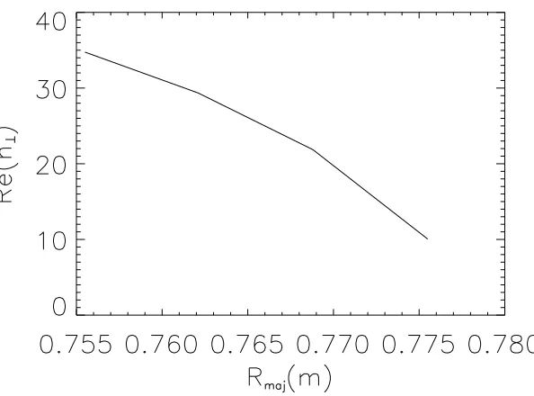
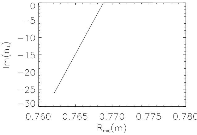
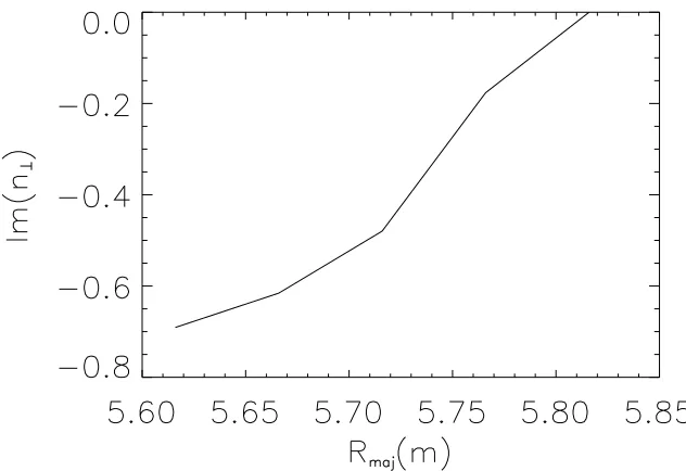
2.4.3 Dispersion Relation for EBWs

We plot the real and imaginary parts of

against \

t

`

\

for three branches of the Electron Bernstein Modes as they pass through the electron cyclotron resonance or an associated harmonic. In the discussion that follow we need to distinguish between the exact resonance and its harmonics where

\

t

`

\ø8 5

5

and the resonant regions surrounding these points. We will thus refer to each of these

points as a cold resonance on the grounds that in the absence of thermal effects these points are the reso-nant regions.

The range of values of

as\

t

`

\

increases corresponds the values the wave takes as it prop-agates from the exterior to the interior of a tokamak and sees an increasing magnetic field and hence

\

t

`

\

This simple model does not account for changes in density and temperature, but remains useful in understanding a wave’s behaviour over a short distance, such as at and around a cyclotron harmonic.

The three modes we plot are capable of co-existing at one value of \

t

`

\

, and the branch ob-tained by our dispersion relation for a particular set of parameters is dependent on the initial guess of

rather than any conscious selection by the person running the program. Building a coherent picture of the modes thus requires that we interpret the results obtained, locating each mode, and then progressing along the particular mode’s dispersion curve in small steps so as not to stray onto another mode.

The general picture is that each branch propagates through the cold resonance it first encounters and the dispersion curve is plotted for this. In reality the wave would be absorbed far too rapidly upon entering the resonant region for this to be observed in any experiment, but it is still informative to con-sider the full range of results, and its costs comparitively little in terms of effort to obtain the results. We also note that our plots only show the waves travelling from low field to high field, but a wave approaching a cyclotron harmonics from the ”right hand side” will still see the resonance and experience resonant damping in the vicinity of the exact resonance. The effects of the resonance on the ”left hand side” of the wave can be seen in later higher temperature cases, but we will discuss this more later.

(42)

Figure 2.4.1 Plots of three branches of the Electron Bernstein Modes:

against t

` around the

fun-damntal cyclotron resonance, and its second and third harmonics.

8

' #"

, ~

8

&

º

, ý

¤

æ+æ

8

!

,

F\

`

\

J

8

¹

Electron cyclotron heating and current drive using the electron Bernstein modes