kNN-IS: An Iterative Spark-based design of the k-Nearest Neighbors Classifier for Big Data
Jesus Maillo, Sergio Ram´ırez, Isaac Triguero, Francisco Herrera
PII: S0950-7051(16)30175-7
DOI: 10.1016/j.knosys.2016.06.012
Reference: KNOSYS 3567
To appear in: Knowledge-Based Systems Received date: 31 January 2016
Revised date: 10 June 2016 Accepted date: 12 June 2016
Please cite this article as: Jesus Maillo, Sergio Ram´ırez, Isaac Triguero, Francisco Herrera, kNN-IS: An Iterative Spark-based design of the k-Nearest Neighbors Classifier for Big Data,Knowledge-Based Systems(2016), doi:10.1016/j.knosys.2016.06.012
ACCEPTED MANUSCRIPT
kNN-IS: An Iterative Spark-based design of the
k-Nearest Neighbors Classifier for Big Data
Jesus Mailloa,∗, Sergio Ram´ıreza, Isaac Trigueroc,d,e, Francisco Herreraa,b
aDepartment of Computer Science and Artificial Intelligence, University of Granada,
CITIC-UGR, Granada, Spain, 18071
bFaculty of Computing and Information Technology, University of Jeddah, Jeddah, Saudi
Arabia, 21589
cDepartment of Internal Medicine, Ghent University, Ghent, Belgium, 9000 dData Mining and Modelling for Biomedicine group, VIB Inflammation Research Center,
Zwijnaarde, Belgium, 9052
eSchool of Computer Science, University of Nottingham, Jubilee Campus, Wollaton
Road, Nottingham NG8 1BB, United Kingdom
Abstract
The k-Nearest Neighbors classifier is a simple yet effective widely renowned method in data mining. The actual application of this model in the big data domain is not feasible due to time and memory restrictions. Several dis-tributed alternatives based on MapReduce have been proposed to enable this method to handle large-scale data. However, their performance can be further improved with new designs that fit with newly arising technologies.
In this work we provide a new solution to perform an exact k-nearest neighbor classification based on Spark. We take advantage of its in-memory operations to classify big amounts of unseen cases against a big training dataset. The map phase computes the k-nearest neighbors in different train-ing data splits. Afterwards, multiple reducers process the definitive neighbors from the list obtained in the map phase. The key point of this proposal lies on the management of the test set, keeping it in memory when possible. Other-wise, it is split into a minimum number of pieces, applying a MapReduce per chunk, using the caching skills of Spark to reuse the previously partitioned
∗Corresponding author. Tel : +34 958 240598; Fax: + 34 958 243317
Email addresses: [email protected](Jesus Maillo),
[email protected](Sergio Ram´ırez),[email protected]
ACCEPTED MANUSCRIPT
training set. In our experiments we study the differences between Hadoop and Spark implementations with datasets up to 11 million instances, showing the scaling-up capabilities of the proposed approach. As a result of this work an open-source Spark package is available.
Keywords: K-nearest neighbors, Big data, Apache Hadoop, Apache Spark, MapReduce
1. Introduction
Over the last few years, gathering information has become an automatic and relatively inexpensive task, thanks to technology improvements. This has resulted in a severe increment of the amount of available data. Social media, biomedicine or physics are just a few examples of areas that are producing tons of data every day [1]. This data is useless without a proper knowledge extraction process that can somehow take advantage of it. This fact poses a significant challenge to the research community because standard machine learning methods can not deal with the volume, diversity and complexity that this data brings [2]. Therefore, existing learning techniques need to be remodeled and updated to deal with such volume of data.
The k-Nearest Neighbor algorithm (kNN) [3] is an intuitive and effective nonparametric model used for both classification and regression purposes. In [4], the kNN was claimed to be one of the ten most influential data mining algorithms. In this work, we are focused on classification tasks. As a lazy learning model, the kNN requires that all the training data instances are stored. Then, for each unseen case and every training instance, it performs a pairwise computation of a certain distance or similarity measure [5, 6], selecting thek closest instances to them. This operation has to be repeated for all the input examples against the whole training dataset. Thus, the application of this technique may become impractical in the big data context. In what follows, we refer to this original algorithm as the exact kNN method, w.r.t. partial and approximate variants of the kNN model that reduce the computational time, assuming that distances are computed using any class of approximation error bound [7].
imple-ACCEPTED MANUSCRIPT
clas-ACCEPTED MANUSCRIPT
sify large amounts of test samples against a big training dataset, avoiding start-up costs of Hadoop. To do so, we read the test set line by line from the Hadoop File System, which make this model fully scalable but its per-formance can be further improved by in-memory solutions.
In this paper, we propose an iterative MapReduce-based approach for kNN algorithm implemented under Apache Spark. In our implementation, we aim to exploit the flexibility provided by Spark, by using other in-memory operations that alleviate the consumption costs of existing MapReduce alter-natives. To manage enormous test sets as well, this method will iteratively address chunks of this set, if necessary. The maximum number of possible test examples, depending on memory limitations, will be used to minimize the number of iterations. In each iteration, a kNN MapReduce process will be applied. The map phase consists of deploying the computation of sim-ilarity between a subset of the test examples and splits of the training set through a cluster of computing nodes. As a result of each map, the class la-bel of the k nearest neighbors together with their computed distance values will be emitted to the reduce stage. Multiple reducers will determine which are the final k nearest neighbors from the list provided by the maps. This process is repeated until the whole test set is classified. Through the text, we will denote this approach as a kNN design based on Spark (kNN-IS).
In summary, the contributions of this work are as follows:
• We extend the MapReduce scheme proposed in [28] by using multiples reducers to speed up the processing when the number of maps needed is very high.
• A fully parallel implementation of the kNN classifier that makes use of in-memory Spark operations to accelerate all the stages of the method, including normalization of the data, processing of big test datasets, and computation of pairwise similarities, without incurring in Hadoop startup costs.
ACCEPTED MANUSCRIPT
The remainder of this paper is organized as follows. Section 2 introduces the big data technologies used in this work and the current state-of-art in kNN big data classification. Then, Section 3 details the proposed kNN-IS model. Section 4 describes the experimental setup and Section 5 includes multiple analyses of results. Finally, Section 6 outlines the conclusions drawn in this work. The Appendix provides a quick start guide with the developed Spark package.
2. Preliminaries
This section provides the necessary background for the remainder of the paper. First, Section 2.1 introduces the concept of MapReduce and the platforms Hadoop and Spark. Then, Section 2.2 formally defines the kNN algorithm and its weaknesses to tackle big data problems, presenting the current alternatives to alleviate them.
2.1. MapReduce Programming Model and Frameworks: Hadoop and Spark The MapReduce programming paradigm [8] is a scale-out data processing tool for Big Data, designed by Google in 2003. This was thought to be the most powerful search-engine on the Internet, but it rapidly became one of the most effective techniques for general-purpose data parallelization.
MapReduce is based on two separate user-defined primitives: Map and Reduce. The Map function reads the raw data in form of key-value (< key, value >) pairs, and transforms them into a set of intermediate< key, value > pairs, conceivably of different types. Both key and value types must be de-fined by the user. Then, MapReduce merges all the values associated with the same intermediate key as a list (shuffle phase). Finally, the Reduce func-tion takes the grouped output from the maps and aggregates it into a smaller set of pairs. This process can be schematized as shown in Figure 1.
This transparent and scalable platform automatically processes data in a distributed cluster, relieving the user from technical details, such as: data partitioning, fault-tolerance or job communication. We refer to [16] for an exhaustive review of this framework and other distributed paradigms.
ACCEPTED MANUSCRIPT
Figure 1: Data flow overview of MapReduce
popularity, Hadoop and MapReduce have shown not to fit well in many cases, like online or iterative computing [31]. Its inability to reuse data through in-memory primitives makes the application of Hadoop for many machine learning algorithms unfeasible.
Apache Spark, a novel solution for large-scale data processing, was thought to be able to solve the Hadoop’s drawbacks [32, 33]. Spark was introduced as part of the Hadoop Ecosystem and it is designed to cooperate with Hadoop, specially by using its distributed file system. This framework proposes a set of in-memory primitives, beyond the standard MapReduce, with the aim of processing data more rapidly on distributed environments, up to 100x faster than Hadoop.
Spark is based on Resilient Distributed Datasets (RDDs), a special type of data structure used to parallelize the computations in a transparent way. These parallel structures let us persist and reuse results, cached in memory. Moreover, they also let us manage the partitioning to optimize data place-ment, and manipulate data using a wide set of transparent primitives. All these features allow users to easily design new data processing pipelines.
ACCEPTED MANUSCRIPT
machine learning algorithms. However, this platform does not include lazy learning algorithms such as the kNN algorithm.
2.2. The kNN classifier and big data
The kNN algorithm is a non-parametric method that can be used for either classification and regression tasks. Here, we define the kNN problem, its current trends and the drawbacks to manage big data. A formal notation for the kNN algorithm is the following:
Let T R be a training dataset and T S a test set, they are formed by a determined number n and t of samples, respectively. Each sample xp is
a tuple (xp1,xp2, ...,xpD, ω), where, xpf is the value of the f-th feature of
the p-th sample. This sample belongs to a class ω, given by xω
p, and a D
-dimensional space. For theT R set the classωis known, while it is unknown for T S. For each sample xtest included in the T S set, the kNN algorithm
searches the k closest samples in the T R set. Thus, the kNN calculates the distances between xtest and all the samples of T R. The Euclidean distance
is the most widely-used measure for this purpose. The training samples are ranked in ascending order according to the computed distance, taking the k nearest samples (neigh1,neigh2, ...,neighk). Then, they are used to compute the most predominant class label. The chosen value of k may influence the performance and the noise tolerance of this technique.
Although the kNN has shown outstanding performance in a wide variety of problems, it lacks the scalability to manage big T R datasets. The main problems found for dealing with large-scale data are:
• Runtime: The complexity to find the nearest neighbor training example of a single test instance isO((n·D)), wherenis the number of training instances andDthe number of features. This becomes computationally more expensive when it involves finding the k closets neighbors, since it requires the sorting of the computed distances, so that, an extra complexity O(n·log(n)). Finally, this process needs to be repeated for every test example.
ACCEPTED MANUSCRIPT
These drawbacks motivate the use of big data technologies to distribute the processing of kNN over a cluster of nodes.
In the literature, we can find a family of approaches that perform kNN joins with MapReduce. A recent review on this topic can be found in [36]. The kNN joins differs from kNN classifier in the expected output. While the kNN classifier aims to provide the predicted class, the kNN join outputs the neighbors themselves for a single test. Thus, these methods cannot be applied for classification.
For an exact kNN join, two main alternatives have been proposed in [25]. The first one, named H-BkNNJ, consists of a single round of MapReduce in whichT RandT S sets are partitioned together, so that, every map task pro-cesses a pairT Si andT Ri, and carries out the pairwise distance comparison
ACCEPTED MANUSCRIPT
single test example, which is very time consuming in both Hadoop and also in Spark (as we will discuss further in the experiment section). The latter was proposed in [28], denoted as MR-kNN, in which a single MapReduce process manages the classification of the (big) test set. To do that, Hadoop primitives are used to read line by line the test data within the map phase. As such, this model is scalable but its performance can be further improved by in-memory solutions.
3. kNN-IS: An Iterative Spark-based design of the kNN classifier for Big Data
In this section we present an alternative distributed kNN model for big data classification using Spark. We will denote our method as kNN-IS. We focus on the reduction of the runtime of the kNN classifier, when both train-ing and test sets are big datasets. As stated in [36], when computtrain-ing kNN within a parallel framework, many additional factors may impact the execu-tion time, such as number of MapReduce jobs j or number of Map m and Reduce rtasks required. Therefore, writing an efficient exact kNN in Spark is challenging, and multiple key-points must be taken into account to obtain an efficient and scalable model.
Aiming to alleviate the main issues presented by previously MapReduce solutions for kNN, we introduce the following ideas in our proposal:
• As in [28] and [27], a MapReduce process will split the training dataset, as it is usually the biggest dataset, into m tasks. In contradistinction to kNN-join approaches that needm2 tasks, we reduce the complexity of kNN to m tasks without requiring any preprocessing in advanced.
• To tackle large test datasets, we rely on Spark to reuse the previously split training set with different chunks of the test set. The use of multiple MapReduce jobs over the same data does not imply significant extra costs in Spark, but we keep this number to a minimum. The MR-kNN approach only performs m tasks independently of the test data size, by reading line-by-line the test set within the maps. Here we show how in-memory operations highly reduce the cost of every task.
ACCEPTED MANUSCRIPT
of reducers, which can be determinant when the size of the dataset becomes very big (See Section 5.3).
• In addition, every single operation will be performed within the RDD objects provided by Spark. It means that even simple operations such as normalization, are also efficient and fully scalable.
This is the reasoning behind our model. In what follows, we detail its main components. First of all, we will present the main MapReduce process that classifies a subset of the test set against the whole training set (Section 3.1). Then, we give a global overview of the method, showing the details to carry out the iterative computation over the test data (Section 3.2).
3.1. MapReduce for kNN classification within Spark
This subsection introduces the MapReduce process that will manage the classification of subsets of test data that fit in memory. As such, this MapRe-duce process is based on our previously proposed alternative MR-kNN, with the distinction that it allows for multiple reducers, checks the iterations re-quired to run avoiding memory swap, and is implemented under Spark.
As a MapReduce model, this divides the computation into two main phases: the map and the reduce operations. The map phase splits the train-ing data and calculates for each chunk the distances and the correspondtrain-ing classes of theknearest neighbors for every test sample. The reduce stage ag-gregates the distances of theknearest neighbors from each map and makes a definitive list ofknearest neighbors. Ultimately, it conducts the usual major-ity voting procedure of the kNN algorithm to predict the resulting class. Map and reduce functions are now defined in Sections 3.1.1 and 3.1.2, respectively.
3.1.1. Map Phase
Let us assume that the training set T R and the corresponding subset of test samples T Si have been previously read from HDFS as RDD
ob-jects. Hence, the training dataset T R has already been split into a user-defined number m of disjoint subsets when it was read. Each map task (M ap1, M ap2, ..., M apm) tackles a subset T Rj, where 1 ≤ j ≤ m, with the
samples of each chunk in which the training set file is divided. Therefore, each map approximately processes a similar number of training instances.
To obtain an exact implementation of kNN, the input test set T Si is not
ACCEPTED MANUSCRIPT
compare every test sample against the whole training set. It implies that bothT Si and T Rj are supposed to fit altogether in memory.
Algorithm 1 Map function
Require: T Rj T Si; k
1: fort= 0 to size(T Si)do
2: CDt,j ← Compute kNN (T Rj, T Si(x), k) 3: resultj ← (< key:t, value:CDt,j >) 4: EMIT(resultj)
5: end for
Algorithm 1 contains the pseudo-code of this function. In our imple-mentation in Spark we make use of themapPartitions(func)transformation, which runs the function defined in Algorithm 1 on each block of the RDD separately.
Every map j will constitute a class-distance vector CDt,j of pairs <
class, distance > of dimension k for each test sample t in T Si. To do so,
Instruction 2 computes for each test sample the class and the distance to its k nearest neighbors. To accelerate the posterior actualization of the nearest neighbors in the reducers, every vector CDt,j is sorted in
ascend-ing order regardascend-ing the distance to the test sample, so that,Dist(neigh1)< Dist(neigh2)< .... < Dist(neighk).
Unlike the MapReduce proposed in [28], every map sends multiple out-puts, e.g. one per test instance. The vector CDt,j is outputted as value
together with an identifier of test instance t as key (Instruction 3). In this way, we allow this method to use multiple reducers. Having more reducers may be useful when the used training and test datasets are very big.
3.1.2. Reduce Phase
The reduce phase consists of collecting, from the tentativeknearest neigh-bors provided by the maps, the closest ones for the examples contained in T Si. After the map phase, all the elements with the same key have been
grouped. A reducer is run over a list(CDt,0, CDt,1, .., CDt,m) and determines
thek nearest neighbors of this test example t.
This function will process every element of such list one after another. Instructions 2 to 7 update a resulting list resultsreducer with the k
ACCEPTED MANUSCRIPT
sorted lists up to get k values, so that, the complexity in the worst case is O(k). Therefore, this function compares every distance value of each of the neighbors one by one, starting with the closest neighbor. If the distance is lesser than the current value, the class and the distance of this position is up-dated with the corresponding values, otherwise we proceed with the following value. Algorithm 2 provides the details of the reduce operation.
In summary, for every instance in the test set, the reduce function will aggregate the values according to function described before. To ease the implementation of this idea, we use the transformation ReduceByKey(func) from Spark. Algorithm 2 corresponds to the function required in Spark.
Algorithm 2 Reduce by key operation
Require: resultkey, k 1: cont=0
2: fori= 0to k do
3: if resultkey(cont).Dist < resultreducer(i).Dist then 4: resultreducer(i) =resultkey(cont)
5: cont++
6: end if
7: end for
3.2. General scheme of kNN-IS
When the size of the test set is very large, we may exceed the memory allowance of the map tasks. In this case, we also have to split the test dataset and carry out multiple iterations of the MapReduce process defined above. Figure 2 depicts the general work-flow of the method. Algorithm 3 shows the pseudo-code of the whole method with precise details of the functions utilized in Spark. In the following, we describe the most significant instructions, enumerated from 1 to 13.
As input, we receive the path in the HDFS for both training and test data as well as the number of maps m and reducers r. We also dispose of the number of neighbors k and the memory allowance for each map.
ACCEPTED MANUSCRIPT
ACCEPTED MANUSCRIPT
Since we will use Euclidean distance to compute the similarity between instances, normalizing both datasets becomes a mandatory task. Thus, In-structions 3 and 4 both perform a parallel operation to normalize the data into the range [0,1]. Both datasets are also cached for future reuse.
Even though Spark can be iteratively applied with the same data without incurring excessive time consumption, we reduce the number of iterations to a minimum because the fewer iterations there are, the better the performance will be. Instruction 5 calculates the minimum number of iterations #Iter that we will have to perform to manage the input data. To do so, it will use the size of every chunk of the training dataset, the size of the test set and the memory allowance for each map.
With the computed number of iterations #Iter, we can easily split the test dataset into subsets of a similar number of samples. To do that, we make use of the previously established keys in T S (in Instruction 2). Instruction 6 will perform the partitioning of the test dataset by using the function RangePartitioner.
Next, the algorithm enters into a loop in which we classify subsets of the test set (Instructions 7-12). Instruction 7 firstly gets the split corresponding to the current iteration. We use the transformation filterByRange(lowKey, maxKey) to efficiently take the corresponding subset. This function takes advantage of the split performed in Instruction 6, to only scan the matching elements. Then, we broadcast this subset T Si into the main memory of all
the computing nodes involved. The broadcast function of Spark allows us to keep a read-only variable cached on each machine rather than copying it with the tasks.
After that, the main map phase starts in Instruction 9. As stated before, themapPartition function computes the kNN for each partitions ofT Rj and
T Si and emits a pair RDD with key equals to the number of instance and
value equals to a list of class-distance. The reduce phase joins the results of each map grouping by key (Instruction 9). As a result, we obtain the k neighbors with the smallest distance and their classes for each test input in T Si. More details can be found in the previous section.
The last step in this loop collects the right and predicted classes storing them as an array in every iteration (Instruction 11).
ACCEPTED MANUSCRIPT
Algorithm 3 kNN-IS
Require: T R; T S;k; #M aps; #Reduces; #M emAllow
1: T R-RDDraw ← textFile(T R, #M aps) 2: T S-RDDraw ← textFile(T S).zipWithIndex() 3: T R-RDD ← T R-RDDraw.map(normalize).cache 4: T S-RDD ← T S-RDDraw.map(normalize).cache
5: #Iter ← calIter(T R-RDD.weight(), T S-RDD.weight, M emAllow)
6: T S-RDD.RangePartitioner(#Iter)
7: fori= 0to #Iterdo
8: T Si ← broadcast(T S-RDD.getSplit(i))
9: resultKNN← T R-RDD.mapPartition(T Rj → kNN(T Rj, T Si,k)) 10: result←resultKN N.reduceByKey(combineResult,#Reduces).collect
11: right-predictedClasses[i] ← calculateRightPredicted(result)
12: end for
13: cm← calculateConfusionMatrix(right-predictedClasses)
4. Experimental set-up
In this section, we show the factors and points related to the experimental study. We provide the performance measures used (Section 4.1), the details of the problems chosen for the experimentation (Section 4.2) and the involved methods with their respective parameters (Section 4.3). Finally, we specify the hardware and software resources that support our experiments (Section 4.4).
4.1. Performance measures
In this work we assess the performance and scalability with the following three measures:
• Accuracy: Represents the number of correct classifications against the total number of classified instances. This is calculated from a resulting confusion matrix, dividing the sum of the diagonal elements between the total of the elements of the confusion matrix. This is the most commonly used metric for assessing the performance of classifiers for years in standard classification ([38] [39]).
ACCEPTED MANUSCRIPT
will take intermediate times from the map phase and the reduce phase to better analyze the behavior of our proposal. The total runtime for the parallel approach includes reading and distributing all the data, in addition to calculating k nearest neighbors and majority vote.
• Speed up: Proves the efficiency of a parallel algorithm comparing against the sequential version of the algorithm. Thus, it measures the relation between the runtime of sequential and parallel versions. In a fully par-allelism environment, the maximum theoretical speed up would be the same as the number of used cores, according to the Amdahl’s Law [40].
Speedup= base line
parallel time (1)
where base line is the runtime spent with the sequential version and parallel time is the total runtime achieved with its improved version.
4.2. Datasets
In this experimental study we will use four big data classification prob-lems. PokerHand, Susy and Higgs are extracted from the UCI machine learn-ing repository [41]. Moreover, we take an extra dataset that comes from the ECBDL’14 competition [42]. This is a highly imbalanced problem (Imbal-anced ratio > 45), in which the kNN may be biased towards the negative class. Thus, we randomly sample said dataset to obtain more balance. The point of using said dataset, is that apart from containing a substantial num-ber of instances, it has a relatively high numnum-ber of features, so that, we can see how this fact affects the proposed model.
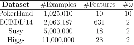
Table 1 summarizes the characteristics of these datasets. We show the number of examples (#Examples), number of features (#F eatures), and the number of classes (#ω). Note that with a fewer number of instances, the ECBLD’14 datasets become the larger datasets in terms of size because of its number of features.
For the experimental study all datasets have been partitioned using a 5 fold cross-validation (5-fcv) scheme. It means that the dataset is partitioned into 5 folds, each one including 80% training samples and the rest test ex-amples. For each fold, the kNN algorithm computes the nearest neighbors from theT S against T R.
ACCEPTED MANUSCRIPT
Table 1: Summary description of the used datasets
Dataset #Examples #Features #ω PokerHand 1,025,010 10 10 ECBDL’14 2,063,187 631 2
Susy 5,000,000 18 2
Higgs 11,000,000 28 2
number of maps is, the fewer number of instances there are in them. Table 2 presents the number of instances in each training set according to the number of maps used. In italics we represent the settings that are not used in our experiments because there are either too few instances or too many.
Table 2: Approximate number of instances in the training subset depending on the number of mappers
Number of maps
Dataset 32 64 128 256 512 1024 2048
PokerHand 25,626 12,813 6,406 3,203 1,602 800 400 ECBDL’14 51,580 25,790 12,895 6,448 3,224 1,612 806 Susy 62,468 31,234 15,617 7,809 3,905 1,953 976 Higgs 275,000 137,500 68,750 34,375 17,188 8,594 4,297
The number of reducers also plays an important role in how the test dataset is managed in kNN-IS. The larger the number of reducers, the smaller the number of test instances that have to be processed for each reducer. Table 3 shows this relation, assuming that the test set is not split because of memory restrictions (so, number of iterations = 1). Once again, we point out in italics those settings that have not been explored.
Table 3: Approximate number of instances in the test subset depending on the number of reducers
Number of reducers
Dataset 1 32 64 128
PokerHand 205,002 102,501 51,250 25,625 ECBDL’14 412,637 12,895 6,448 3,224
ACCEPTED MANUSCRIPT
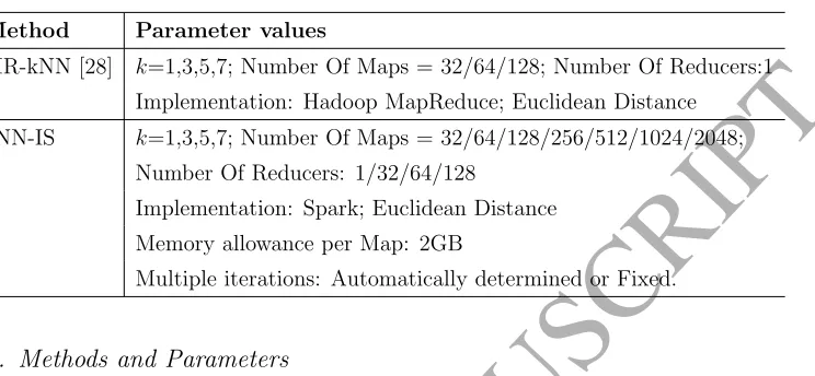
Table 4: Parameter settings for the used methods.
Method Parameter values
MR-kNN [28] k=1,3,5,7; Number Of Maps = 32/64/128; Number Of Reducers:1
Implementation: Hadoop MapReduce; Euclidean Distance
kNN-IS k=1,3,5,7; Number Of Maps = 32/64/128/256/512/1024/2048;
Number Of Reducers: 1/32/64/128
Implementation: Spark; Euclidean Distance Memory allowance per Map: 2GB
Multiple iterations: Automatically determined or Fixed.
4.3. Methods and Parameters
Among the existing distributed kNN models based on MapReduce, we establish a comparison with the model proposed in [28], MR-kNN, as the most promising alternative proposed so far, which is based in Hadoop MapReduce. As stated in Section 2.2, kNN-join methods [36] were originally designed for other purposes rather than classification. They also require the data size to increase and even a squared number of Map tasks. Therefore, their theoretical complexity is so much higher than the proposed technique that we have discarded a comparison of such models, as it would be very time consuming.
We have also conducted preliminary experiments in order to apply the iterative method proposed iHMR-kNN [27]. However, the iterative processing becomes so slow that we have not been able to apply it to any of the datasets considered in a timely manner.
This work is mainly devoted to testing the scalability capabilities of the proposed model, showing how it palliates the weaknesses of previously pro-posed models stated in Section 2.2. To do so, we will analyze the effect of the number of neighbors, and the number of maps and reducers. Table 4 summarizes the parameters used for both MR-kNN and kNN-IS models.
4.4. Hardware and software used
ACCEPTED MANUSCRIPT
• Processors: 2x Intel Xeon CPU E5-2620
• Cores: 6 cores (12 threads)
• Clock speed: 2 GHz
• Cache: 15 MB
• Network: Infiniband (40Gb/s)
• RAM: 64 GB
The specific details of the software used and its configuration are the following:
• MapReduce implementations: Hadoop 2.6.0-cdh5.4.2 and Spark 1.5.1
• Maximum number of map tasks: 256
• Maximum number of reduce tasks: 128
• Maximum memory per task: 2GB.
• Operating System: Cent OS 6.5
Note that the total number of available cores is 192, which becomes 384 by using hyper-threading technology. Thus, when we explore a number of maps greater than 384, we cannot expect linear speedups, since there will be queued tasks. For these cases, we will focus on analyzing the map and reduce runtimes.
5. Analysis of results
In this section, we study the results collected from different experimental studies. Specifically, we analyze the next four points:
• First, we establish a comparison between kNN-IS and MR-kNN (Sec-tion 5.1).
ACCEPTED MANUSCRIPT
• Third, we check the impact of the number of reducers in relation to the number of maps when tackling very large datasets (Section 5.3).
• Finally, we study the behavior of kNN-IS with huge test datasets, in which the method is obliged to perform multiple iterations (Section 5.4).
5.1. Comparison with MR-kNN
This section compares kNN-IS with MR-kNN, as the potentially fastest alternative proposed so far. To do this, we make use of PokerHand and Susy datasets. We could not go further than these datasets in order to obtain the results of the sequential kNN. In these datasets, kNN-IS only needs to conduct one iteration, since the test datasets fits in the memory in a every map. The number of reducers in kNN-IS has been also fixed to 1, to establish a comparison between very similar MapReduce alternatives under Hadoop (MR-kNN) or Spark (kNN-IS).
First of all, we run the sequential version of kNN over these datasets as a baseline. As in [28], this sequential version reads the test set line by line, as done by MR-kNN, as a straightforward solution to avoid memory problems. We understand that this scenario corresponds to the worst possible case for the sequential version, and better sequential versions could be designed. However, our aim here is to compare with the simplest sequential version, assuming that large test sets do not fit in memory together with the training set.
Table 5 shows the runtime (in seconds) and the average accuracy (Ac-cTest) results obtained by the standard kNN algorithm, depending on the number of neighbors.
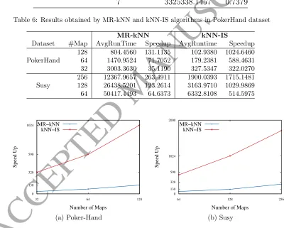
Table 6 summarizes the results obtained with both methods with k=1. The next Section will detail the influence of the value of k. It shows, for each number of maps (#Maps) the average total time (AvgRuntime) and the speedup achieved against the sequential version. As stated before, both methods correspond to exact implementation of the kNN, so that, we obtain exactly the same average accuracy as presented in Table 5.
Figure 3 plots speed up comparisons of both approaches against the se-quential version as the number of maps is increased (k = 1).
ACCEPTED MANUSCRIPT
Table 5: Sequential kNN performance
Dataset Number of Neighbors Runtime(s) AccTest 1 105475.0060 0.5019
PokerHand 3 105507.8470 0.4959
5 105677.1990 0.5280 7 107735.0380 0.5386 1 3258848.8114 0.6936
Susy 3 3259619.4959 0.7239
5 3265185.9036 0.7338 7 3325338.1457 0.7379
Table 6: Results obtained by MR-kNN and kNN-IS algorithms in PokerHand dataset
MR-kNN kNN-IS
Dataset #Map AvgRunTime Speedup AvgRuntime Speedup
128 804.4560 131.1135 102.9380 1024.6460
PokerHand 64 1470.9524 71.7052 179.2381 588.4631
32 3003.3630 35.1190 327.5347 322.0270
256 12367.9657 263.4911 1900.0393 1715.1481
Susy 128 26438.5201 123.2614 3163.9710 1029.9869
64 50417.4493 64.6373 6332.8108 514.5975
0 130 320 590 1024
32 64 128
Speed Up
Number of Maps MR−kNN
kNN−IS
(a) Poker-Hand
0 130 320 590 1024 2000
64 128 256
Speed Up
Number of Maps MR−kNN
kNN−IS
(b) Susy
Figure 3: Speedup comparisons between MR-kNN and kNN-IS against the sequential kNN
ACCEPTED MANUSCRIPT
However, Table 6 shows how this runtime can be greatly reduced in both approaches as the number of maps is increased. As stated above, both alternatives always provide the same accuracy as the sequential version.
• According to Figure 3, a linear speed up for the hadoop-based kNN model has been achieved since both models read the test dataset set line-by-line, which is sometimes even superlinear what is related to memory-consumption problems of the original kNN model to manage the training set. However, kNN-IS presents a faster speed up than a linear speed up in respect to this sequential version. This is because of the use of in-memory data structures that allowed us to avoid reading test data from HDFS line-by-line.
• Comparing MR-kNN and kNN-IS, the results show how Spark has al-lowed us to reduce the runtime needed almost 10-fold in comparison to Hadoop.
5.2. Influence of the number of neighbors
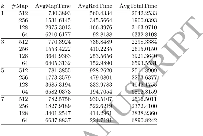
To deeply analyze the influence of the number of neighbors we focus on the Susy dataset, and we set the number of reducer tasks to one again. We analyze its effect in both map and reduce phases.
Table 7 collects for each number of neighbors (#Neigh) and number of maps (#Maps), the average map execution time (AvgMapTime), the average reduce time (AvgRedTime) and the average total runtime (AvgTotalTime). Recall that in our cluster the maximum number of map tasks is set to 256. Thus, the total runtime for 512 maps does not show a linear reduction, but it can be appreciated in the reduction of the map runtime.
Figure 4 presents how the value ofkinfluences in map runtimes. It depicts the map runtimes in terms of number of maps fork = 1,3,5 and 7. Figure 5 plots the reduce runtime in relation to thek value and number of maps.
According to these tables and plots, we can conclude that:
ACCEPTED MANUSCRIPT
700 1500 3500 6500
64 128 256 512
Map Runtime (in seconds)
Number of Maps 1 3 5 7
Figure 4: Influence of parameterkin the map phase: Susy dataset
150 300 550 800
64 128 256 512
Reduce Runtime (in seconds)
Number of Maps 1 3 5 7
ACCEPTED MANUSCRIPT
Table 7: Results obtained with Susy dataset
k #Map AvgMapTime AvgRedTime AvgTotalTime
1 512 730.3893 560.4334 2042.2533
256 1531.6145 345.5664 1900.0393
128 2975.3013 166.3976 3163.9710
64 6210.6177 92.8188 6332.8108
3 512 770.3924 736.8489 2298.3384
256 1553.4222 410.2235 2615.0150
128 3641.9363 253.5656 3921.3640
64 6405.3132 152.9890 6593.5531
5 512 781.3855 928.2620 2511.8909
256 1773.3579 479.0801 2273.6377
128 3685.3194 332.9783 4042.1755
64 6582.0373 194.7054 6802.8159
7 512 782.5756 930.5107 2516.5011
256 1827.9189 522.6219 2372.4100
128 3401.2547 414.2961 3838.2360
64 6637.8837 224.7191 6890.8242
• Comparing Figures 4 and 5, we can see that the number of neighbors seem to have more influence on the reduce runtime than on the map phase. This is because the number of neighbors does not affect the main computation cost (computing the distances between test and training instances) of the map phase, while it may affect the updating process performed in the reducers since its complexity is O(k).
Finally, as a general appreciation, Figure 5 reveals that when a larger number of maps is used, which is clearly necessary to deal big datasets, the reduce runtimes increase considerably. This has motivated the study carried out in the next Section.
5.3. Influence of the number of reducers
As we just saw in the previous section, a high number of maps greatly increases the load of the reduce phase. However, the use of a large number of maps may be absolutely necessary to tackle very big datasets. This section investigates how the proposed idea of managing different test instances in multiple reducers may help to alleviate such an issue.
ACCEPTED MANUSCRIPT
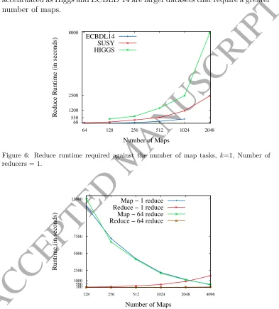
Figure 6 plots the reduce time required with a single reducer for all these problems. It confirms, as pointed out in the previous section, the drastic increment when the number of maps is very high. It is actually even more accentuated as Higgs and ECBLD’14 are larger datasets that require a greater number of maps.
60 550 1200 2500 8000
64 128 256 512 1024 2048
Reduce Runtime (in seconds)
Number of Maps ECBDL14
SUSY HIGGS
Figure 6: Reduce runtime required against the number of map tasks, k=1, Number of reducers = 1.
100 500 1000 2500 5000 7500 13000
128 256 512 1024 2048 4096
Runtime (in seconds)
Number of Maps Map − 1 reduce Reduce − 1 reduce Map − 64 reduce Reduce − 64 reduce
ACCEPTED MANUSCRIPT
100 500 1000 2500 6000
64 128 256 512 1024 2048
Runtime (in seconds)
Number of Maps Map − 1 reduce Reduce − 1 reduce Map − 64 reduce Reduce − 64 reduce
Figure 8: Map and Reduce runtimes required according to the number of maps - SUSY
100 500 2000 5000 10000 15000 20000
128 256 512 1024 2048
Runtime (in seconds)
Number of Maps Map − 1 reduce Reduce − 1 reduce Map − 64 reduce Reduce − 64 reduce
ACCEPTED MANUSCRIPT
[image:28.595.143.489.217.437.2]For sake of clarity, we do not present the associated tables of results for the three considered problems, but we visually present such results in Figures 7, 8 and 9. These figures plot the map and reduce runtimes spent in ECBLD’14, Susy and Higgs, respectively, in terms of the number of maps and reduces utilized.
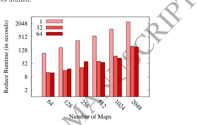
2 8 32 128 512 2048
64 128 256 512 1024 2048
Reduce Runtime (in seconds)
Number of Maps 1
32 64
Figure 10: Reduce Runtime vs. number of maps and reducers — SUSY
These figures reveal that:
• Using multiple reducers effectively softens the runtime spent in the reduce phase when it is necessary to use a larger number of maps. In the previous plots, we can see how the version with a single reducer rapidly increases its computational cost in comparison to the version with more reducers.
• The reduction in the required time is not linear in respect to the number of reducers. As pointed out in [43], an excessive number of reducers can also lead to a MapReduce overhead in the network. As we can see, for example in Figure 10, there are no great differences when using 32 or 64 reducers.
ACCEPTED MANUSCRIPT
for the Susy dataset, it is not convenient to use more than 32 reducers unless we have more than 512 maps.
In conclusion, it is important to find a trade-off between the number of maps and reducers according to the cluster and the dataset that we dispose.
5.4. Dealing with large amounts of test data
To test the behavior of the full model presented here, we carry out a study in which both training and test sets are composed of the same number of instances. In this way, we ensure that kNN-IS is obliged to perform multiple iterations. To do so, we test training versus training datasets.
Table 8 presents the results of the three datasets with more than one iteration (#Iter), average reduce runtime (AvgRedTime) and the average total runtime (AvgTotalTime). To study the influence of test size, we focus on k=1, with 256 maps, 64 reduces for Susy and ECBDL’14 datasets and 128 reduce tasks for the Higgs dataset (#Red).
Table 8: Results obtained with more than one iteration.
Dataset #Iter AvgMapTime AvgRedTime AvgTotalTime
ECBDL’14 3 7309.7122 8.8911 28673.7015
#Red=64 5 4303.7106 5.2520 28918.2992
10 2027.5685 2.8076 29121.0583
SUSY 2 2385.6183 34.2682 6723.7762
#Red=64 5 1156.9453 14.1350 9493.5098
10 649.7218 5.9823 10278.2612
HIGGS 2 16835.6982 144.3371 44414.1423
#Red=128 5 7145.7838 59.3202 46806.8294
10 3668.4418 29.7266 51836.9468
Figure 11 presents the influence of the number of iterations. The ECBDL’14 dataset needs 3 iterations to fit the main memory. The other datasets only need 2 iterations. Figure 11a shows the map time with a different number of iterations for the three datasets used. Figure 11b presents how the number of iterations influences the reduce runtimes and Figure 11c plots the total runtime versus the number of iterations.
Analyzing these tables and plots, we can observe that:
ACCEPTED MANUSCRIPT
500 2000 4000 7000 16000
2 3 5 10
Runtime (in seconds)
Number of Iterations ECBDL14
Susy Higgs
(a) Map Runtime
2 10 40 140
2 3 5 10
Runtime (in seconds)
Number of Iterations ECBDL14
Susy Higgs
(b) Reduce Runtime
6000 10000 30000 40000 50000
2 3 5 10
Runtime (in seconds)
Number of Iterations ECBDL14
Susy Higgs
(c) Total Runtime
Figure 11: Runtimes vs Number of Iterations
• However, Figure 11c shows how it slightly increases the total runtime. This behavior could be caused by a network saturation of the cluster. For ECBDL’14 dataset, the total runtime increases less than other two datasets. This happens because it has fewer samples as shown in Table 1. Thus, it produces less network traffic in spite of having more features.
ACCEPTED MANUSCRIPT
6. Conclusions and further work
In this paper we have developed a Iterative MapReduce solution for the k-Nearest Neighbors algorithm based on Spark. It is denominated as kNN-IS. The proposed scheme is an exact model of the kNN algorithm that we have enabled to apply with large-datasets. Thus, kNN-IS obtains the same accuracy as kNN. However, the kNN algorithm has two main issues when dealing with large-scale data: Runtime and Memory consumption. The use of Apache Spark has provided us with a simple, transparent and efficient environment to parallelize the kNN algorithm as an iterative MapReduce process.
The experimental study carried out has shown that kNN-IS obtains a very competitive runtime. We have tested its behavior with datasets of different sizes (different number of features and different number of samples).
The main achievements obtained are the following:
• kNN-IS is an exact parallel approach and obtains the same accuracy and very good achievements on runtimes.
• kNN-IS (Spark) has allowed us to reduce the runtime needed by almost 10 times in comparison to MR-kNN (Hadoop).
• Despite producing more transfer from the map to reduce, the number of neighbors (k) does not drastically affect to the total runtime.
• We can optimize the runtime with a trade-off between the number of maps and reducers according to the cluster and the dataset used
• When datasets are enormous and it exceed the memory capacity of the cluster, kNN-IS calculates the solution with more than one iteration by splitting the test set. Therefore, it has allowed us to apply the kNN algorithm in large-scale problems.
• The software of this contribution can be found as a spark-package at
http://spark-packages.org/package/JMailloH/kNN_IS. The source
code of this technique can be found in the next repository https: //github.com/JMailloH/kNN_IS
ACCEPTED MANUSCRIPT
of features by using multi-view approaches. We are planning to extend the use of kNN-IS to instance selection techniques for big data [45], where it reports good results. Another direction for future work is to extend the application of the presented kNN-IS approach to a big data semi-supervised learning [46] context.
APPENDIX
As consequence of this work, we have developed a Spark package with the kNN-IS implementation. It has all the functionalities exposed in this study. In addition, we have developed kNN-IS for the machine learning library on Spark, as part of the MLlib library and the MLbase platform.
Prerequisites: You must have Spark 1.5.1, Scala 2.10 and Maven 3.3.3 or higher installed. Java Virtual Machine 1.7.0 is necessary because Scala runs over it.
The implementation allows us to determine the:
• Number of Cores to be used: Number of cores to compute the MapRe-duce approach.
• Number of neighbors: Number of neighbors. The value of k.
• Number of maps: Number of map tasks.
• Number of reduces: Number of reduce tasks.
• Number of iterations: Number of iterations. Setting to -1 to auto-setting the iterations. We give optional parameter (Maximum memory per node) limit on GB for each map task. This selects the minimum number of iterations within the limit provided.
The input data is expected to be in KEEL Dataset format [47]. The datasets are previously stored in HDFS.
The output will be stored in HDFS in the following format: ./output-Path/Predictions.txt/part-00000 contains the predicted and right class in two column. ./outputPath/Result.txt/part-00000 shows confusion matrix, accu-racy and total runtime. ./outputPath/Times.txt/part-00000 presents higher map time, higher reduce time, average iterative time and total runtime.
ACCEPTED MANUSCRIPT
The proposed kNN-IS is now available as a Spark Package at http:// spark-packages.org/package/JMailloH/kNN_IS
Acknowledgments
This work has been supported by the Spanish National Research Project TIN2014-57251-P and the Andalusian Research Plan P11-TIC-7765. J. Maillo and S. Ram´ırez hold FPU scholarships from the Spanish Ministry of Educa-tion. I. Triguero held a BOF postdoctoral fellowship from Ghent University during part of the development of this work.
References
[1] C. Lynch, Big data: How do your data grow?, Nature 455 (7209) (2008) 28–29. doi:10.1038/455028a.
[2] M. Minelli, M. Chambers, A. Dhiraj, Big Data, Big Analytics: Emerging Business Intelligence and Analytic Trends for Today’s Businesses (Wiley CIO), 1st Edition, Wiley Publishing, 2013.
[3] T. M. Cover, P. E. Hart, Nearest neighbor pattern classification, IEEE Transactions on Information Theory 13 (1) (1967) 21–27.
[4] X. Wu, V. Kumar (Eds.), The Top Ten Algorithms in Data Mining, Chapman & Hall/CRC Data Mining and Knowledge Discovery, 2009.
[5] Y. Chen, E. K. Garcia, M. R. Gupta, A. Rahimi, L. Cazzanti, Similarity-based classification: Concepts and algorithms, Journal of Machine Learning Research 10 (2009) 747–776.
[6] K. Q. Weinberger, L. K. Saul, Distance metric learning for large margin nearest neighbor classification, Journal of Machine Learning Research 10 (2009) 207–244.
[7] S. Arya, D. M. Mount, N. S. Netanyahu, R. Silverman, A. Y. Wu, An optimal algorithm for approximate nearest neighbor searching fixed di-mensions, J. ACM 45 (6) (1998) 891–923. doi:10.1145/293347.293348.
ACCEPTED MANUSCRIPT
[9] S. Ghemawat, H. Gobioff, S.-T. Leung, The google file system, in: Pro-ceedings of the nineteenth ACM symposium on Operating systems prin-ciples, SOSP ’03, 2003, pp. 29–43.
[10] C. P. Chen, C.-Y. Zhang, Data-intensive applications, challenges, tech-niques and technologies: A survey on big data, Information Sciences 275 (2014) 314 – 347. doi:10.1016/j.ins.2014.01.015.
[11] Z. Guo, G. Fox, M. Zhou, Investigation of data locality in mapre-duce, in: Cluster, Cloud and Grid Computing (CCGrid), 2012 12th IEEE/ACM International Symposium on, 2012, pp. 419–426. doi:10.1109/CCGrid.2012.42.
[12] A. Srinivasan, T. Faruquie, S. Joshi, Data and task parallelism in ILP using mapreduce, Machine Learning 86 (1) (2012) 141–168.
[13] I. Triguero, S. del R´ıo, V. L´opez, J. Bacardit, J. M. Ben´ıtez, F. Herrera, ROSEFW-RF: The winner algorithm for the ecbdl’14 big data competi-tion: An extremely imbalanced big data bioinformatics problem, Know.-Based Syst. 87 (C) (2015) 69–79. doi:10.1016/j.knosys.2015.05.027.
[14] X. Yan, J. Zhang, Y. Xun, X. Qin, A parallel algorithm for mining constrained frequent patterns using mapreduce, Soft Computing (2015) 1–13doi:10.1007/s00500-015-1930-z.
[15] W. Gropp, E. Lusk, A. Skjellum, Using MPI: portable parallel program-ming with the message-passing interface, Vol. 1, MIT press, 1999.
[16] A. Fern´andez, S. R´ıo, V. L´opez, A. Bawakid, M. del Jesus, J. Ben´ıtez, F. Herrera, Big data with cloud computing: An insight on the computing environment, mapreduce and programming frameworks, WIREs Data Mining and Knowledge Discovery 4 (5) (2014) 380–409.
[17] K. Grolinger, M. Hayes, W. Higashino, A. L’Heureux, D. Allison, M. Capretz, Challenges for mapreduce in big data, in: Services (SERVICES), 2014 IEEE World Congress on, 2014, pp. 182–189. doi:10.1109/SERVICES.2014.41.
ACCEPTED MANUSCRIPT
Conference on Uncertainty in Artificial Intelligence (UAI), Catalina Is-land, California, 2010.
[19] Y. Bu, B. Howe, M. Balazinska, M. D. Ernst, Haloop: Efficient iterative data processing on large clusters, Proc. VLDB Endow. 3 (1-2) (2010) 285–296. doi:10.14778/1920841.1920881.
[20] M. Zaharia, M. Chowdhury, T. Das, A. Dave, J. Ma, M. McCauley, M. J. Franklin, S. Shenker, I. Stoica, Resilient distributed datasets: A fault-tolerant abstraction for in-memory cluster computing, in: Proceed-ings of the 9th USENIX conference on Networked Systems Design and Implementation, USENIX Association, 2012, pp. 1–14.
[21] M. Ghesmoune, M. Lebbah, H. Azzag, Micro-batching growing neu-ral gas for clustering data streams using spark streaming, Proce-dia Computer Science 53 (2015) 158 – 166, INNS Conference on Big Data 2015 Program San Francisco, CA, USA 8-10 August 2015. doi:10.1016/j.procs.2015.07.290.
[22] I. Triguero, D. Peralta, J. Bacardit, S. Garc´ıa, F. Herrera, MRPR: A mapreduce solution for prototype reduction in big data clas-sification, Neurocomputing 150, Part A (0) (2015) 331 – 345. doi:10.1016/j.neucom.2014.04.078.
[23] S. D. M. Du, H. Jia, Study on density peaks clustering based on k-nearest neighbors and principal component analysis, Knowledge-Based Systems 99 (2016) 135 – 145. doi:10.1016/j.knosys.2016.02.001.
[24] D. C. M. Z. Z. Deng, X. Zhu, S. Zhang, Efficient knn classification algorithm for big data, Neurocomputing 195 (2016) 143 – 148, learning for Medical Imaging. doi:10.1016/j.neucom.2015.08.112.
[25] C. Zhang, F. Li, J. Jestes, Efficient parallel knn joins for large data in mapreduce, in: Proceedings of the 15th International Conference on Ex-tending Database Technology, EDBT ’12, ACM, New York, NY, USA, 2012, pp. 38–49. doi:10.1145/2247596.2247602.
ACCEPTED MANUSCRIPT
[27] K. Sun, H. Kang, H.-H. Park, Tagging and classifying facial images in cloud environments based on kNN using mapreduce, Optik - Interna-tional Journal for Light and Electron Optics 126 (21) (2015) 3227 – 3233. doi:10.1016/j.ijleo.2015.07.080.
[28] J. Maillo, I. Triguero, F. Herrera, A mapreduce-based k-nearest neighbor approach for big data classification, in: 9th International Conference on Big Data Science and Engineering (IEEE BigDataSE-15), 2015, pp. 167– 172.
[29] T. White, Hadoop: The Definitive Guide, 3rd Edition, O’Reilly Media, Inc., 2012.
[30] A. H. Project, Apache hadoop (2015).
URLhttp://hadoop.apache.org/
[31] J. Lin, Mapreduce is good enough? if all you have is a hammer, throw away everything that’s not a nail!, Big Data 1:1 (2013) 28–37.
[32] H. Karau, A. Konwinski, P. Wendell, M. Zaharia, Learning Spark: Lightning-Fast Big Data Analytics, O’Reilly Media, Incorporated, 2015.
[33] A. Spark, Apache Spark: Lightning-fast cluster computing, [Online; ac-cessed July 2015] (2015).
URLhttps://spark.apache.org/
[34] A. Spark, Machine Learning Library (MLlib) for Spark, [Online; ac-cessed May 2016] (2016).
URLhttp://spark.apache.org/docs/latest/mllib-guide.html
[35] A. Spark, Machine Learning Library (ML) for Spark, [Online; accessed May 2016] (2016).
URLhttp://spark.apache.org/docs/latest/ml-guide.html
[36] G. Song, J. Rochas, F. Huet, F. Magoules, Solutions for processing k nearest neighbor joins for massive data on mapreduce, in: Parallel, Dis-tributed and Network-Based Processing (PDP), 2015 23rd Euromicro In-ternational Conference on, 2015, pp. 279–287. doi:10.1109/PDP.2015.79.
ACCEPTED MANUSCRIPT
[38] E. Alpaydin, Introduction to Machine Learning, 2nd Edition, The MIT Press, 2010.
[39] I. H. Witten, E. Frank, Data Mining: Practical Machine Learning Tools and Techniques, Second Edition (Morgan Kaufmann Series in Data Management Systems), Morgan Kaufmann Publishers Inc., San Fran-cisco, CA, USA, 2005.
[40] G. M. Amdahl, Validity of the single processor approach to achieving large scale computing capabilities, in: Proceedings of the April 18-20, 1967, Spring Joint Computer Conference, AFIPS ’67 (Spring), ACM, New York, NY, USA, 1967, pp. 483–485. doi:10.1145/1465482.1465560.
[41] M. Lichman, UCI machine learning repository (2013).
URLhttp://archive.ics.uci.edu/ml
[42] ECBDL14 dataset: Protein structure prediction and contact map for the ECBDL2014 big data competition (2014).
URLhttp://cruncher.ncl.ac.uk/bdcomp/
[43] C.-T. Chu, S. Kim, Y.-A. Lin, Y. Yu, G. Bradski, A. Ng, K. Olukotun, Map-reduce for machine learning on multicore, in: Advances in Neural Information Processing Systems, 2007, pp. 281–288.
[44] J. Luengo, S. Garc´ıa, F. Herrera, On the choice of the best imputation methods for missing values considering three groups of classification methods, Knowledge and Information Systems 32 (1) (2011) 77–108. doi:10.1007/s10115-011-0424-2.
[45] J. R. ´A. Arnaiz-Gonz´alez, J.F. D´ıez-Pastor, C. Garc´ıa-Osorio, Instance selection of linear complexity for big data, Knowledge-Based Systems (2016) –doi:10.1016/j.knosys.2016.05.056.
[46] I. Triguero, S. Garc´ıa, F. Herrera, Self-labeled techniques for semi-supervised learning: taxonomy, software and empirical study, Knowledge and Information Systems 42 (2) (2013) 245–284. doi:10.1007/s10115-013-0706-y.