Global navigation satellite systems performance analysis and augmentation strategies in aviation

Global navigation satellite systems

performance analysis and augmentation strategies in aviation

Roberto Sabatini

*

, Terry Moore

and Subramanian Ramasamy

1_{RMIT University, School of Engineering – Aerospace Engineering and Aviation Discipline, Bundoora, VIC 3083, Australia} 2_{University of Nottingham, Nottingham Geospatial Institute, Nottingham, NG7 2TU, United Kingdom}

A B S T R A C T

In an era of significant air traffic expansion characterised by a rising congestion of the radiofrequency spectrum and a widespread introduction of Unmanned Aircraft Systems (UAS), Global Navigation Satellite Systems (GNSS) are being exposed to a variety of threats including signal interferences, adverse propagation effects and challenging platform-satellite relative dynamics. Thus, there is a need to characterize GNSS signal degradations and assess the effects of interfering sources on the performance of avionics GNSS receivers and augmentation systems used for an increasing number of mission-essential and safety-critical aviation tasks (e.g., experimental flight testing, flight inspection/certification of ground-based radio navigation aids, wide area navigation and precision approach). GNSS signal deteriorations typically occur due to antenna obscuration caused by natural and man-made obstructions present in the environment (e.g., elevated terrain and tall buildings when flying at low altitude) or by the aircraft itself during manoeuvring (e.g., aircraft wings and empennage masking the on-board GNSS antenna), ionospheric scintillation, Doppler shift, multipath, jamming and spurious satellite transmissions. Anyone of these phenomena can result in partial to total loss of tracking and possible tracking errors, depending on the severity of the effect and the receiver characteristics. After designing GNSS performance threats, the various augmentation strategies adopted in the Communication, Navigation, Surveillance/Air Traffic Management and Avionics (CNS+A) context are addressed in detail. GNSS augmentation can take many forms but all strategies share the same fundamental principle of providing supplementary information whose objective is improving the performance and/or trustworthiness of the system. Hence it is of paramount importance to consider the synergies offered by different augmentation strategies including Space Based Augmentation System (SBAS), Ground Based Augmentation System (GBAS), Aircraft Based Augmentation System (ABAS) and Receiver Autonomous Integrity Monitoring (RAIM). Furthermore, by employing multi-GNSS constellations and multi-sensor data fusion techniques, improvements in availability and continuity can be obtained. SBAS is designed to improve GNSS system integrity and accuracy for aircraft navigation and landing, while an alternative approach to GNSS augmentation is to transmit integrity and differential correction messages from ground-based augmentation systems (GBAS). In addition to existing space and ground based augmentation systems, GNSS augmentation may take the form of additional information being provided by other on-board avionics systems, such as in ABAS. As these on-board systems normally operate via separate principles than GNSS, they are not subject to the same sources of error or interference. Using suitable data link and data processing technologies on the ground, a certified ABAS capability could be a core element of a future GNSS Space-Ground-Aircraft Augmentation Network (SGAAN). Although current augmentation systems can provide significant improvement of GNSS navigation performance, a properly designed and flight-certified SGAAN could play a key role in trusted autonomous system and cyber-physical system applications such as UAS Sense-and-Avoid (SAA).

1. Introduction

The origins of Global Navigation Satellite Systems (GNSS) date back to the early 1960s, when the United States Department of Defense initiated the development of systems for three– dimensional position determination [1]. After the US Navy successfully tested the first satellite navigation system called TRANSIT, the Space Division of the US Air Force initiated a program, known as Project 621B that evolved into the Navigation Signal Time and Range (NAVSTAR) program. In 1973, the US Defense Navigation Satellite System (DNSS) was created, which was later referred to as NAVSTAR Global Positioning System (GPS). Various GNSS systems are currently in service or under development. The US GPS and the Russian GLONASS (Globalnaya Navigazionnaya Sputnikovaya Sistema) have achieved their Full Operational Capability (FOC) back in the 1990’s [2]. Other GNSS systems that are currently at the advanced development or deployment stages include the European GALILEO and the People’s Republic of China BEIDOU Navigation Satellite System (BDS). GNSS systems typically use signals 20 dB below the ambient noise floor and, despite several research efforts devoted to interference detection and mitigation strategies at receiver and platform level (mostly for military applications), no effective solution has been implemented so far in the civil aviation context. Thus, there is a need to characterize GNSS signal degradations and assess the effects of interfering sources on the performance of avionics GNSS receivers and Differential GNSS (DGNSS) systems used for an increasing number of mission-essential and safety-critical aviation tasks (e.g.,

experimental flight testing, flight inspection/certification of ground-based radio navigation aids, wide area navigation and precision approach).

GNSS signal deteriorations typically occur due to antenna obscuration caused by natural and man-made obstructions present in the environment (e.g., elevated terrain and tall buildings when flying at low altitude) or by the aircraft itself during manoeuvring (e.g., aircraft wings and empennage masking the on-board GNSS antenna), ionospheric scintillation, Doppler shift, multipath, jamming and spurious satellite transmissions. Anyone of these phenomena can result in partial to total loss of tracking and possible tracking errors, depending on the severity of the effect and the receiver characteristics. Tracking errors, especially if undetected by the receiver software, can result in large position errors. Partial loss of tracking results in geometry degradation, which in turn affects position accuracy. Consequently, GNSS alone does not always provide adequate performance in mission-essential and safety-critical aviation applications where high levels of accuracy and integrity are required.

GNSS augmentation can take many forms but all share the same fundamental principle of providing supplementary information whose objective is improving the performance and/or trustworthiness of the system. GNSS augmentation benefits in the aviation domain can be summarized as follows:

 Increased runway access, more direct en-route flight paths and new precision approach services;

 Potential elimination of some ground-based navigation aids (VOR, ILS, etc.) with cost saving to Air Navigation Service Providers (ANSPs).

This paper is organised as follows: Section 2 provides a detailed discussion on GNSS aviation applications, followed by a description of models for GNSS performance threats in Section 3; Section 4 presents the different augmentation strategies and the identification of a pathway to a future GNSS Space-Ground-Avionics Augmentation Network (SGAAN) is discussed in Section 5; an investigation of the potential of GNSS augmentation techniques to support trusted autonomous Unmanned Aircraft System (UAS) applications is presented in Section 6; The conclusions of this article are summarised in Section 7 and recommendations for future research are highlighted in Section 8.

2. GNSS Aviation Applications

Although different GNSS systems employ diversified hardware and software features, all systems are composed by a space segment, a control segment and a user segment (Fig. 1). The space segment includes the satellites required for global coverage. These satellites are predominantly in Intermediate Circular Orbit (ICO),

at nominal altitudes of 19,100 km (GLONASS), 20,184 km (GPS) and 23,222 km (GALILEO) from the Earth’s surface.

BDS also employs satellites in Geostationary Orbit (GEO) and Inclined Geosynchronous Orbit (IGSO). The user segment includes the large variety of GNSS receivers developed for air, ground and marine navigation positioning applications. The control segment includes one or more Control and Processing Stations (CPSs) connected to a number of Ground Monitoring Stations (GMSs) and antennae located around the globe for Telemetry, Tracking and Command (TT&C) signals down/uplink and navigation/integrity signals uplink to the satellites. The GMS antennae passively track all GNSS satellites in view collecting ranging signals from each satellite. This information is passed on to the CPS where the satellite ephemeris and clock parameters are estimated and predicted. Additionally, satellite integrity data are analysed and appropriate integrity flags are generated for faulty/unreliable satellites. The ephemeris/clock and integrity data are then up-linked to the satellite for retransmission in the navigation message. The satellite clock drift is corrected so that all transmitted data are synchronised with GNSS time.

Space Segment

Control Segment

User Segment

Satellite TT&C Data

Navigation/Integrity Data Satellite Navigation Signals

Constellation Monitoring Data

Ground Monitoring Station

Satellite TT&C Link

Navigation/Integrity Uplink Control/Processing Station

Legend:

Fig. 1. GNSS segments.

The fundamental equation is the following:

ݐீேௌௌ=ݐ௦−߂ݐ௦ (1)

whereݐ_ீேௌௌis the GNSS time,ݐ_௦is the satellite time and߂ݐ_௦is the difference between satellite and GNSS time. The corrections are applied to the last term of equation (1), typically using polynomial coefficients and a relativistic correction term. The correction equation can be written as:

߂ݐ௦=ܽ଴+ܽଵ(ݐீேௌௌ−ݐ଴௖) +ܽଶ(ݐீேௌௌ−ݐ଴௖)ଶ+߂ݐ௥ (2)

whereܽ_଴, ܽ_ଵ and ܽ_ଶare the polynomial coefficients for phase, frequency and age offset;߂ݐ_௥is the relativistic correction term and

ݐ଴௖is the time of transmission of the corrections.

Typically, the ephemeris corrections are obtained through an estimation of the Cartesian co-ordinates of the satellites along the orbits by integrating the equations of motion. For integrity purposes, suitable Fault Detection, Isolation and Recovery (FDIR) techniques are employed. In particular, the health status of the satellite subsystems is continuously monitored (satellite payload, bus, solar arrays, battery power and the level of propellant used for maneuvers) and any anomaly must be promptly detected and resolved. When needed, spare satellites can be activated. The

Signal-in-Space (SIS) is also constantly monitored to guarantee the required performance standards. Despite the significant technological enhancements recently introduced in control segment integrity features, current GNSS systems have limited FDIR capability. In most cases, several minutes or even hours are required to provide the required integrity information (i.e., use/do not use signals) to GNSS users. Obviously, this is not acceptable for mission-essential and safety-critical aviation applications.

2.1. GNSS Observables

combinations of the original phase observation, such as double differences and triple differences.

2.1.1. Pseudorange Observable

The concept of pseudoranging is based on measuring difference between the time of transmission of the code from the satellite and the epoch of reception of the same signal at the receiver antenna. This is achieved by correlating identical pseudorandom noise (PRN) codes generated by the satellite’s clock, with those generated internally by the receiver’s own clock. If this time difference is multiplied by the speed of propagation of the radio wave, a range value is obtained which is the distance between the satellite and the receiver’s antenna referring to the epoch of observation. Both receiver and satellite clock errors affect the pseudoranges. Therefore, they differ from the actual geometric distance corresponding to the epochs of emission and reception. The general pseudorange equation is:

ܲ௞௣(ݐ௞) = (ݐ௞−ݐ௣) ×ܿ (3)

where ܲ_௞௣ represents the actual measurement, ݐ_௞ denotes the nominal time of the receiver clock݇at reception,ݐ௣denotes the nominal time of the satellite clock݌at emission andܿdenotes the speed of light. Equation (3) would correspond to the actual distance between the satellite and receiver’s antenna, if there were no clock biases, the signal travelled through vacuum and there was no multipath effect. The clock drifts can be represented by the following expressions:

ݐ௥,௞=ݐ௞+݀ݐ௞ (4)

ݐ௞௣=ݐ௣+݀ݐ௣ (5)

where the symbolݎdenotes the true time and the terms݀ݐ_௞and

݀ݐ௣_{are the receiver and satellite clock errors respectively. Taking}

these errors and biases into account, the complete expression for the pseudorange becomes:

ܲ௞௣(ݐ௞) =൫ݐݎ,݇−ݐݎ݌൯ܿ− (݀ݐ௞ −݀ݐ௣)ܿ+ܫ௞,௣௣(ݐ௞)+ ܶ௞௣(ݐ௞)+݀௞,௣(ݐ௞) +݀௞,௣௣(ݐ௞) +݀௣௣(ݐ௞) +ߝ௣ (6)

Therefore,

ܲ௞௣(ݐ௞) =ߩ௞௣(ݐ௥,௞) − (݀ݐ௞ −݀ݐ௣)ܿ+ܫ௞,௣௣(ݐ௞)+ ܶ௞௣(ݐ௞)+݀௞,௣(ݐ௞) +݀௞,௣௣(ݐ௞) +݀௣௣(ݐ௞) +ߝ௣ (7)

whereܫ_௞,௣௣(ݐ_௞)and

 

T are the ionospheric and tropospheric delays, depending on varying conditions along the path of the signal. The symbols ݀_௞,௣(ݐ_௞)and݀_௣௣(ݐ_௞)denote the receiver and satellite hardware code delays respectively. The symbol

݀௞,௣௣(ݐ௞)denotes the multipath of the codes, which depends on

the geometry of the antenna and satellite with respect to surrounding reflective surfaces. The termߝ_௣denotes the random measurement noise. The term ߩ_௞௣(ݐ_௥,௞) is the actual geometric distance between the receiver’s antenna and the satellite at a specific epoch and therefore:

ߩ௞௣(ݐ௥) =ඥ(ݑ݌−ݑ݇)2+ (ݒ݌−ݒ݇)2+ (ݓ݌−ݓ݇)2 (8)

The terms (ݑ_௞,ݒ_௞,ݓ_௞)are the approximate Cartesian co-ordinates of the receiver and (ݑ௣,ݒ௣,ݓ௣)denote the position of the satellite at the epoch of transmission. With reference to Fig. 2, assuming a constant receiver clock error݀ݐ_௞for measurements to any satellite and omitting all other error terms in Eq. (6), the following system of equations is formed:

⎩ ⎪ ⎨ ⎪

⎧ܲ௞ଵ(ݐ) =ඥ(ݑଵ−ݑ௞)ଶ+ (ݒଵ−ݒ௞)ଶ+ (ݓଵ−ݓ௞)ଶ−ܿ݀ݐ௞ ܲ௞ଶ(ݐ) =ඥ(ݑଶ−ݑ௞)ଶ+ (ݒଶ−ݒ௞)ଶ+ (ݓଶ−ݓ௞)ଶ−ܿ݀ݐ௞ ܲ௞ଷ(ݐ) =ඥ(ݑଷ−ݑ௞)ଶ+ (ݒଷ−ݒ௞)ଶ+ (ݓଷ−ݓ௞)ଶ−ܿ݀ݐ௞ ܲ௞ସ(ݐ) =ඥ(ݑସ−ݑ௞)ଶ+ (ݒସ−ݒ௞)ଶ+ (ݓସ−ݓ௞)ଶ−ܿ݀ݐ௞

(9)

Therefore, the co-ordinates of the user receiver (and GNSS time) can be derived from the simultaneous observation of four (or more) satellites. If more than four satellites are visible, a least-square solution can be determined. The GNSS receiver calculates its position in an Earth-Centred Earth Fixed (ECEF) Cartesian co-ordinate system (typically using WGS84). These co-co-ordinates may be expressed to some other system such as latitude, longitude and altitude if desired. Solution of the system (equation 9) requires measurement of the pseudoranges to four different satellites. The GNSS receiver’s computer may be programmed to solve directly the navigation equations in the form given above. However, the computation time required to solve them may be too long for many applications.

O h Re

 

(xk, yk, zk)

(x2_{, y}2_{, z}2₎

(x3_{, y}3,_z3₎

XE _Y

E ZE

(x4_{, y}4_{, z}4₎

(x1_{, y}1_{, z}1₎

Greenwitch Meridian

Equator North Pole

Fig. 2. Navigation solution in the ECEF co-ordinate system (at time zero, the XEaxis passes through the North Pole, and the YEaxis completes the

right-handed orthogonal system.

As an alternate approach, these equations may be approximated by a set of four linear equations that the GPS receiver can solve using a much faster and simpler algorithm. The system of equations (9) can be rewritten in the form:

ܲ௞௜(ݐ) =ඥ(ݑ݅−ݑ݇)2+ (ݒ݅−ݒ݇)2+ (ݓ݅−ݓ݇)2+ܶ (10)

(i = 1, 2, 3, 4)

whereݑ௜,ݒ௜andݓ௜represent the co-ordinates of the ith satellite,

ܶ= ݀ݐ݇and the units have been chosen so that the speed of light

is unity. Linearization of equation (10) can proceed as described in [3, 4]. The resulting set of linearized equations relates the pseudorange measurements to the desired user navigation information as well as the user’s clock bias:

ቀ௨೙ି௨೔

௣೙೔ି்೙ቁ∆ݑ௞+ቀ

௩೙ି௩೔

௣೙೔ି்೙ቁ∆ݒ௞+ቀ

௪೙ି௪೔

௣೙೔ି்೙ቁ∆ݓ௞+∆ܶ= ∆ܲ௜(11)

(i = 1, 2, 3, 4)

whereݑ_௡,ݒ_௡,ݓ_௡,ܶ_௡are the nominal (a priori best-estimate) values ofݑ_௞,ݒ_௞,ݓ_௞ andܶ;∆ݑ_௞, ∆ݒ_௞, ∆ݓ_௞, ∆ܶare the corrections to the nominal values;݌_௡௜is the nominal pseudorange measurement to theith_{satellite;∆ܲ}

௜is the difference between actual and nominal

time bias. The coefficients of the quantities on the left-hand side represent the direction cosines of the LOS vector from the user to the satellite as projected along the Cartesian co-ordinate system.

2.1.2. Carrier Phase Observable

The carrier phase observable is the difference between the received satellite carrier phase and the phase of the carrier generated by the receiver oscillator. The same error sources that affect pseudoranges, are responsible for the errors which determine the positional accuracy achieved with carrier phases [5]. Clearly, the mathematical formulation of any specific error component is different from the pseudorange case (i.e., phase measurement errors instead of range measurement errors). Since the antenna cannot sense the number of whole carrier waves between the satellite and the receiver (called the integer ambiguity), an extra parameter is inserted in the carrier phase equation:

ߔ_௞௣=ߔ௞(ݐ)−ߔ௣(ݐ) +ܰ௞௣+ܫ௞௣,ః(ݐ)− ݂ ܿܶ௞௣(ݐ)

+݀௞,ః(ݐ) +݀௞௣,ః(ݐ) +݀௞௣(ݐ) +ߝః (12)

The symbols ߔ_௞(ݐ)andߔ௣(ݐ) denote the phase of the receiver generated signal and the phase of the satellite signal respectively, at the epoch t of satellite signal reception. The symbolܰ_௞௣ is the integer ambiguity. The termsܫ_௞௣_,ః(ݐ)andܶ_௞௣(ݐ)are the ionospheric and tropospheric delays. The ionospheric delay factor has a negative value because the carrier phase progresses when travelling through the ionosphere. Furthermore, the tropospheric factor is converted in cycles multiplying by ݂/ܿ,where݂is the nominal frequency and c is the speed of light in vacuum. The symbols

݀௞,ః(ݐ) and ݀௞௣(ݐ) refer to the receiver and satellite hardware

delays respectively. The symbol ݀_௞௣_,ః(ݐ) denotes the multipath effect and ߝ_ః denotes the carrier phase measurement noise. Assuming synchronisation of the satellite and receiver clocks, omitting other error sources (receiver phase tracking circuits, local oscillator, multipath and measurement noise), and taking into account both the time of transmission and reception of the signal, the equation for the phase observation between a satelliteiand a receiver A, can be written as [6]:

ߔ஺௜(߬) =ߔ௜(ݐ)−ߔ஺(߬) (13)

whereߔ_஺௜(߬)is the phase reading (phase at receiverAof the signal from satelliteiat time߬);ߔ௜(ݐ)is the received signal (phase of the signal as it left the satellite at timet) andߔ_஺(߬)is the generated signal phase (phase of the receiver’s signal at time߬). Ifߩ_஺௜(ݐ) is the range between receiver and satellite, we have:

ݐ=߬−ఘಲ೔(௧)

௖ (14)

Therefore:

ߔ௜_{(ݐ) =ߔ}௜_൬߬−ఘಲ೔(௧)

௖ ൰ (15)

ߔ௜_{(ݐ) =ߔ}௜_(߬)−డః೔(௧) ௗ௧ ถ

௙

×ఘಲ೔(௧)

௖ + ⋯ (16)

ߔ௜_{(ݐ) =ߔ}௜_(߬)−݂×ఘಲ೔(௧)

௖ + ⋯ (17)

and finally:

ߔ஺௜(߬) =ߔ௜(߬)−௙_௖ߩ஺௜(ݐ)−ߔ஺(߬) +ܰ஺௜ (18)

whereߔ_஺௜(߬)is the phase reading (degree or cycles);ߔ௜(߬)is the emitted signal;௙

௖ߩ஺௜(ݐ)is the total number of wavelengths;ߔ஺(߬)

is the generated signal andܰ_஺௜is the integer ambiguity. The carrier phase measurement technique typically uses the difference

between the carrier phases measured at a reference receiver and a user receiver. This is therefore an inherently differential technique.

2.1.3. Doppler Observable

The equation that associates the transmitted frequency from the satellite with the received frequency is:

݂௞= ௙

೛

ଵାೝᇲ_೎ (19)

where ݂_௞ is the received frequency, ݂௣denotes the emitted frequency from the satellite,ݎ′denotes the radial velocity in the satellite-receiver direction and ܿdenotes the speed of light in vacuum. The Doppler frequency shift is given by the difference݂௣−݂_௞. The radial velocity r’ is the actual rate of change in the satellite-receiver distance and it is given by:

ݎᇱ_{= −}௙ೖି௙೛

௙ೖ ∙ܿ (20)

The integrated Doppler count between two epochs ݐ_ଵ andݐ_ଶ is given by:

ܰ(௧భ,௧మ)=∫ (݂௣−݂௞)݀ݐ ௧మ

௧భ (21)

More information about the Doppler observable and on some of its practical uses can be found in the literature [7, 8].

2.2. GNSS Error Sources

In the following paragraphs, the error sources affecting pseudorange and carrier phase measurements are described. The error sources can be classified into the five broad categories as listed below:

 Receiver Dependent Errors: Clock Error, Noise and Resolution;

 Ephemeris Prediction Errors;

 Satellite Dependent Errors: Clock Offset and Group Delays;

 Propagation Errors: Ionospheric Delay, Tropospheric Delay and Multipath;

 User Dynamics Errors.

2.2.1. Receiver Dependent Errors

Most receivers employ quartz clocks to measure GNSS time, which are not as accurate as the atomic clocks of the satellites. Therefore, there is an offset between the receiver and satellite clocks called receiver clock error. This error affects both the measurement of the signal flight time and the calculation of the satellite’s position at time of transmission. Measurement Noise is a random error, which depends entirely on the electronic components of the receiver. Receivers for very precise measurements are designed to minimise this error. Both noise and resolution errors can be reduced by using appropriate filtering techniques. Theoretically, receiver noise can be removed by averaging the measurements, but only over fairly long periods of observation time.

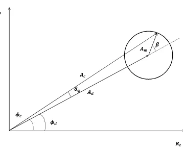
2.2.2. Ephemeris Prediction Errors

In general, the error can be expressed as a function of the three components, in the form:

ܧܴܴ=ܴܣܦܿ݋ݏߙ+ܣܶܭݏ݅݊ߙܿ݋ݏߚ+ܺܶܭݏ݅݊ߙݏ݅݊ߚ (22)

whereߙis the angle between the LOS user-satellite and the satellite vertical andߚis the angle between the ATK direction and the plane containing the LOS and the satellite vertical. The US DoD precise ephemeris is calculated from actual observation to the satellites from a network of ground stations distributed around the world. It is produced several days after the observation period and is available only to authorised users. Other non-DoD organisations produce precise ephemeris, both globally and locally, by suitable modelling of all forces and moments acting on the satellites. Orbit relaxation techniques can be developed within GNSS software. These techniques solve for orbital errors in the broadcast ephemeris and produce improved relative positioning [9-12].

2.2.3. Satellite Dependent Errors

Corrections to the drift of the satellite atomic clocks are computed by the CPS and then broadcasted to the users in the navigation message. The effect of satellite clock offset is negligible in most positioning applications (using the polynomial coefficients corrections computed at the CPS it is possible to reduce this error down to 1 part per 1012_{). The residual error is due to the fact that}

corrections from the CPS are periodic and not continuous. Group Delays are the delays typical of the satellite electronic circuits. They are estimated on the ground before the satellites are launched and corrections are included in the navigation message.

RAD

XTK ATK



Rs

Ru



LOS

Fig. 3.Error components in ephemeris estimation.

2.2.4. Propagation Errors

As discussed, propagation errors include both ionospheric and tropospheric delays. As the satellite signal passes through the ionosphere, it is delayed for two reasons [13]. Firstly, because it travels through a non-vacuum material (propagation delay); thus the Pseudo Random Noise (PRN) codes are delayed, while the carrier phase is advanced when passing through the ionospheric layers. Secondly, because it bends due to refraction; for many applications, the error caused by the bending effect can be considered negligible if the signals are transmitted by satellites with an elevation of 15° or more. The ionospheric delay is dependent primarily on the number of electrons that the signal encounters along its propagation path. It is therefore dependent both on the ionosphere characteristics (variable during the day and with seasons), and the path angle (elevation angle of the satellite). It is possible to approximately evaluate the ionospheric delay using the following equation [13]:

∆߬= 40.31்ா஼_௖௙మ (23)

whereܶܧܥis the total electron content integrated along the LOS to the satellite in units of electrons/m2_{,݂is the frequency in Hz and} ܿis the speed of light. TEC varies with time and depends on the location of the ionosphere ‘pierced’ by the LOS to the satellite. At the L1 frequency (1575.42 MHz), equation (23) can be written for a satellite that is not at the zenith [14]:

∆߬= 0.162ி∙்ா஼ೡ_௖ (24)

whereܶܧܥ_௩is theܶܧܥvalue for a vertical column located at the pierce point, in units of 1016 electrons per m2_{andܨis the obliquity}

factor. Assuming that the active region of the ionosphere can be represented by a thin shell at an elevation of 350 km, the obliquity can be approximately expressed as a simple function of the elevation angle in degrees (ܧ) of the satellite at the receiver’s antenna [14]:

ܨ= 1 + 2.74 ∙ 10ି଺_{(96 −ܧ)}ଷ ₍₂₅₎

Depending on the receiver design, different models can be adopted to calculate the correction terms to be applied to the pseudorange before solving the navigation equations. Particularly, L1 code-range receivers use a sinusoidal model of the ionosphere (called Klobuchar model), which takes into account the variations of the ionospheric layers (low over night, rapidly getting higher after dawn, getting slightly higher during the afternoon and rapidly getting lower after sunset). The sinusoidal parameters (amplitude and period) are transmitted in the navigation message. The relevant equations are the following [15]:

ܫܦܸ=ܦܥ+ܣܿ݋ݏቂଶగ(௧ିః_௉ )ቃ(݀ܽݕ) (26)

ܫܦܸ=ܦܥ(݊݅݃ℎݐ) (27)

representing a model of the ionosphere with varying latitude. As the delay also depends on obliquity of the path, elevation is included as an additional factor in the equation:

ܶܫܦ= [1 + 16(0.53 −ܧ௛)ଷ]ܫܦܸ (28)

where ܶܫܦ is the Total Ionospheric Delay (nsec) and ܧ_௛ is the elevation angle of the satellites over the horizon. As the ionosphere is dispersive at radio frequencies, two signals at different frequencies will be delayed by different amounts. Therefore, double frequency GNSS receivers (e.g., GPS P-code receivers) can measure the difference (Δܶ) between the time of reception of L1 (1575.42 MHz) and L2 (1227.60 MHz), and evaluate the delay associated with both of them. For L1 we have:

∆߬௅ଵ= Δܶ൤ቀ௙ಽభ_௙ಽమቁ ଶ

− 1൨ିଵ (29)

where:

∆ܶ=ସ଴.ଷଵ_௖௙∙మ்ா஼ቀ ଵ ௙_ಽమమ −

ଵ

௙_ಽభమቁ (30)

The troposphere is the lower part of the atmosphere (up to about 50 km) and its characteristics depend on local humidity, temperature and altitude. The tropospheric delay for a given slant range can be described as a product of the delay at the zenith and a mapping function, which models the elevation dependence of the propagation delay. In general, the total Slant Tropospheric Delay (STD) is given by the sum of a Slant Hydrostatic Delay (SHD) and a Slant Wet Delay (SWD), and both of them can be expressed by a relevant Zenith Tropospheric Delay (ZTD) and a Mapping Function (MF). The SHD (or “dry component”) account for about 90% of the total tropospheric delay and accurate estimations are normally available. On the other hand, the “wet component” (SWD) estimations are generally less accurate and there is a significant variability depending on the actual models implemented. Table 1 shows some typical values of the tropospheric delay for various elevation angles [13].

Table. 1. Tropospheric delay for varying elevation angle.

Elevation Angle [°] Dry Component [m] Wet Component [m]

90 2.3 0.2

30 4.6 0.4

10 13.0 1.2

5 26.0 2.3

The total STD is given by:

ܵܶܦ =ܵܪܦ+ܹܵ ܦ (31)

ܵܶܦ=ܼܪܦ×ܯ ܨு+ܼܹ ܦ×ܯ ܨௐ (32)

whereܼܪܦandܼܹ ܦare the zenith hydrostatic delay and zenith wet delay, respectively (ܼܶܦ=ܼܪܦ+ܼܹ ܦ);ܯ ܨ_ு andܯ ܨ_ௐ are their correspondingܯ ܨݏ. There are manyܼܶܦmodels andܯ ܨݏ currently used in GNSS positioning applications. Popular models include theܼܶܦempirical models developed by Saastamoinen [16 and 17], Hopfield [18 and 19] and by the University of New Brunswick [20]. Popular MFs include the ones described by Chao [21], Ifadis [22], Herring [23], Niell [24], and Boehm [25].

2.2.5. Multipath Errors

GNSS signals may arrive at the receiver antenna via different paths, due to reflections by objects along the path. Such effect is known as multipath. The reflected signal will have a different path length compared to the direct signal; therefore, it will give a biased distance measurement (Fig. 4). Multipath depends on the environment surrounding the receiver and on the satellite geometry. Typically, multipath will be greater for low elevation

satellites and code multipath is much greater than carrier phase multipath [26]. For code measurements, the multipath error can reach a theoretical value of 1.5 times the chip rate. So, for instance, the GPS C/A code chip rate is 293.1 metre and the maximum multipath error is about 439.65 metres. However, values of less than 2-3 metres are the norm and upper values of 15 metres are rarely observed. For carrier phase, the maximum theoretical multipath error is a quarter of the wavelength. This equates to about 5 centimetres for the GPS L1 and L2 frequencies, although typical values are less than 1 centimetre [27]. Multipath can be accurately modelled and removed only at static points, by taking observations at the same points and at the same hour on consecutive days. This, however, is possible in a dynamic environment. Other techniques use Signal-to-Noise Ratio (SNR) and signal phase/frequency information to detect and quantify multipath.

Direct Signal Multipath

Signal

GNSS Antenna

Fig. 4. Multipath error.

Despite several technological advances and research efforts addressing multipath detection and mitigation techniques, this is still a major error source in GNSS applications. Techniques such as the Narrow Correlator [28], the Double Delta/Strobe Correlator [29], or the Vision Correlator by Fenton and Jones [30], are not capable of eliminating the multipath-related errors completely.

2.2.6. User Dynamics Error

There are various errors due to the dynamics of a GNSS receiver. These errors range from the physical masking of the GNSS antenna to the accuracy degradation caused by sudden accelerations of the antenna. If carrier phase is used, the resulting effect of “cycle slips” is the need for re-initialisation (i.e., re-determination of the integer ambiguities). In general, a distinction is made between medium-low and high dynamic platforms.

2.3. UERE Vector

receivers is typically less than 20 metres, with the actual value dominated by ionospheric and multipath effects. Dual-frequency receivers (with the capability of removing almost entirely the ionospheric errors), typically experience smaller UEREs. Users of the new modernised GPS civilian signals, as well as future users of GALILEO and BEIDOU, will be able to use multiple frequencies to compensate for the ionospheric errors and thereby to achieve lower UEREs. In GNSS systems the UERE values are strongly dependent on the time elapsed since the last upload from the control segment. As an example, Fig. 5 shows the GPS Standard Positioning Service (SPS) UERE variation with time [31]. In GPS normal operations, the time since last upload is limited to no more than one day. The smallest UERE and best SIS accuracy will generally occur immediately after an upload of fresh NAV message data to a satellite, while the largest UERE and worst SIS accuracy will usually be with the stalest NAV message data just prior to the next upload to that satellite.

Days Since Last Upload 2

0 4 6 8 10 12 14 16 18

Not to scale

100 200 300 400 Extended Operations Normal Operations U E R E (9 5 % ), m

Fig. 5.UERE variation with time in normal and extended operations [31].

The metric used to characterize whether the NAV message data being transmitted by a satellite is fresh or stale is the age of data (AOD), where the AOD is the elapsed time since the control segment generated the satellite clock/ephemeris prediction used to create the NAV message data upload. The AOD is approximately equal to the time since last upload plus the time it took the Control Segment to create the NAV message data and upload it to the satellite. For Normal Operations (NOP), the GPS UERE budget and the traditional SPS SIS accuracy specifications apply at each AOD. Because the largest UERE and worst SIS accuracy usually occur with the oldest NAV message data, the UERE budget and traditional SPS SIS accuracy specifications are taken as applying at the maximum AOD. For reference, the GPS UERE budgets for SPS receivers at zero AOD, at maximum AOD in normal operations, and at 14.5 day AOD in extended operations, are shown in Table 2. The breakout of the individual segment components of the UERE budgets shown in this table is given for illustration purposes only assuming average receiver characteristics. The actual GPS SPS ranging accuracy standards are better specified in terms of the UEE and URE components and the overall error budget is dependent on a number of assumptions, conditions and constraints. Table 3 lists the error budgets and typical UEE values applicable to airborne C/A-code GPS receivers in normal operating conditions. Table 4 lists the condition and criteria that apply to the URE budgeting.

2.4. DOP Factors

Ranging errors alone do not determine GNSS positioning accuracy. The accuracy of the navigation solution is also affected by the relative geometry of the satellites and the user. This is described by the Dilution of Precision (DOP) factors. The four linearized

equations represented by Eq. (9) can be expressed in matrix notation as: ൦ ߂ܲଵ ߂ܲଶ ߂ܲଷ ߂ܲସ

൪=൦

ߚଵଵ ߚଵଶ ߚଵଷ 1

ߚଶଵ ߚଶଶ ߚଶଷ 1

ߚଷଵ ߚଷଶ ߚଷଷ 1

ߚସଵ ߚସଶ ߚସଷ 1

൪൦ ߂ݑ௞ ߂ݒ௞ ߂ݓ ߂ܶ

൪+൦

Єଵ

Єଶ

Єଷ

Єସ

൪ (33)

where an error vector has been added to account for pseudorange measurement noise plus model errors and any unmodelled effects (e.g., SA), andߚ_௜௝is the direction cosine of the angle between the LOS to theith_{satellite and thej}th_co-ordinate.

Table 2.GPS single frequency C/A code UERE budget. Adapted from [31].

Segment Error Source

UERE Contribution [95%][m]

Zero AOD Max AOD in NOP 14.5 Day AOD Space Clock Stability Group Delay Stability

Differential Group Delay Stability

Satellite Acceleration Uncertainty Other Space Segment

Errors 0.0 3.1 0.0 0.0 1.0 8.9 3.1 0.0 2.0 1.0 257 3.1 0.0 204 1.0 Control Clock/Ephemeris Estimation Clock/Ephemeris Prediction Clock/Ephemeris Curve Fit

Iono Delay Model Terms

Group Delay Time Correction

Other Control Segment Errors 2.0 0.0 0.8 9.8-19.6 4.5 1.0 2.0 6.7 0.8 9.8-19.6 4.5 1.0 2.0 206 1.2 9.8-19.6 4.5 1.0 User Ionospheric Delay Compensation Tropospheric Delay Compensation Receiver Noise and

Resolution Multipath

Other User Segment Errors N/A 3.9 2.9 2.4 1.0 N/A 3.9 2.9 2.4 1.0 N/A 3.9 2.9 2.4 1.0

95% System UERE (SPS) 12.7-21.2

17.0-24.1 388

Table. 3. Typical UEE error budget (95%). Adapted from [31].

Error Source Traditional Spec., Single Freq. Rr Improved Spec., Single Freq. Rr Modern Single Freq. Rr Modern Dual Freq. Rr* Ionospheric Delay Compensation

N/A N/A N/A 0.8

Tropospheric Delay Compensation

3.9 4.0 3.9 1.0

Receiver Noise

and Resolution 2.9 2.0 2.0 0.4

Multipath 2.4 0.5 0.2 0.2

UEE [m], 95% 5.5 4.6 4.5 1.6

*Assuming benign conditions [31]

Table 4. SPS SIS URE accuracy standards. Adapted from [31].

SIS Accuracy Standard Conditions and Constraints

Single-Frequency C/A-Code: ≤ 7.8 m 95% Global Average

URE during Normal Operations over all AODs ≤ 6.0 m 95% Global Average

URE during Normal Operations at Zero AOD ≤ 12.8 m 95% Global Average

URE during Normal Operations at Any AOD

For any healthy SPS SIS

Neglecting single-frequency ionospheric delay model errors

Including group delay time correction errors at L1

Including inter-signal bias (P(Y)-code to C/A-(P(Y)-code) errors at L1

Single-Frequency C/A-Code:

 ≤ 30 m 99.94% Global Average URE during Normal

Operations

 ≤ 30 m 99.79% Worst Case Single Point Average

URE during Normal Operations

For any healthy SPS SIS

Neglecting single-frequency ionospheric delay model errors

Including group delay time correction errors at L1

Including inter-signal bias (P(Y)-code to C/A-(P(Y)-code) errors at L1

Standard based on measurement interval of one year; average of

daily values within the service volume

Standard based on 3 service failures per year, lasting no more

than 6 hours each

Single-Frequency C/A-Code:

 ≤ 388 m 95% Global Average URE during Extended Operations after 14

Days without Upload

For any healthy SPS SIS

Equation (33) can be written more compactly as:

ݎ=ܤݔҧ+ Є (34)

whereܤis the 44 solution matrix (i.e., matrix of coefficients of the linear equation); ݔҧis the user position and time correction vector ݔҧ≡ [߂ݑ_௞߂ݒ_௞߂ݓ߂ܶ]்; ݎ is the pseudorange measurement difference vector (ݎ≡ [߂ܲ_ଵ߂ܲ_ଶ߂ܲ_ଷ߂ܲ_ସ]்) andЄ is the vector of measurement and other errors (Є

≡ [ЄଵЄଶ Єଷ Єସ]்).

The GNSS receiver (or post-processing software) solves the matrix equation using least squares or a Kalman Filter (KF). The solution is:

ݔҧ= −(ܤ்_{ܹ ܤ)}ିଵ_ܤ்_ܹ

௥ (35)

The new term in the above equation is the weight matrix (ܹ) that characterizes the differences in the errors of the simultaneous measurements as well as any correlations that may exist among them. The weight matrix is given by:

ܹ =ߪ଴ଶܥ௥ (36)

whereܥ_௥is the covariance matrix of the pseudorange errors and

ߪ଴ଶis a scale factor known as the a priori variance of unit weight.

Applying the law of propagation of error (also known as the covariance law), we obtain:

ܥ௫̅= [(ܤ்ܹ ܤ)ିଵܤ்ܹ]ܥ௥[(ܤ்ܹ ܤ)ିଵܤ்ܹ]் (37)

ܥ௫̅=൫ܤ்ܥ௥ିଵܤ൯ିଵ (38)

whereܥ_௫̅is the covariance matrix of the parameter estimates. If we assume that the measurement and model errors are the same for all

observations with a particular standard deviation (ߪ) and that they are uncorrelated, we can write:

ܥ௥=ܫߪଶ (39)

whereܫis the identity matrix. Therefore, the expression forܥ_௫̅ simplifies to:

ܥ௫̅= (ܤ்ܤ)ିଵߪ௥ଶ=ܦߪ௥ଶ (40)

The term r represents the standard deviation of the pseudorange measurement error plus the residual model error, which is assumed to be equal for all simultaneous observations. If we further assume that the measurement error and the model error components are all independent, then we can simply root-sum-square these errors to obtain the value ofߪ_௥. Based on the definition of UERE given above, we can use the 1-sigma UERE for ߪ_௥. The elements of matrix D are a function of receiver-satellite geometry only. The explicit form of this matrix is:

ܦ=൦

ܦଵଵ ܦଵଶ ܦଵଷ ܦଵସ

ܦଶଵ ܦଶଶ ܦଶଷ ܦଶସ

ܦଷଵ ܦଷଶ ܦଷଷ ܦଷସ

ܦସଵ ܦସଶ ܦସଷ ܦସସ

൪ (41)

The DOP factor can be defined as follows:

ܦܱܲௗ =ඥܶݎܽܿ݁ௗܦ (݀= 1, 2, 3, 4) (42)

wheredis the dimension of the DOP factor. The diagonal elements of C_୶ത are the estimated receiver coordinate and clock-offset variances, and the off-diagonal elements (i.e., covariances) indicate the degree to which these estimates are correlated. The explicit form of theC_୶തmatrix is:

ܥ௫̅=

⎣ ⎢ ⎢ ⎢

⎡ߪ௨ଶ ߪ௨௩ ߪ௨௪ ߪ௨்

ߪ௩௨ ߪ௩ଶ ߪ௩௪ ߪ௩்

ߪ௪ ௨ ߪ௪ ௩ ߪ௪ଶ ߪ௪ ்

ߪ்௨ ߪ்௩ ߪ்௪ ߪ்ଶ⎦

⎥ ⎥ ⎥ ⎤

(43)

The various DOP values can be expressed as functions of the diagonal elements of theܥ_௫̅matrix or of theܦmatrix. Converting the Cartesian co-ordinates in matrix form to more convenient local geodetic coordinates, we have:

ܥ௅ீതതതത=

⎣ ⎢ ⎢

⎡ߪேଶ ߪோ ߪேு ߪே்

ߪாே ߪாଶ ߪாு ߪா்

ߪுே ߪுா ߪுଶ ߪு்

ߪ்ே ߪ்ா ߪ்ு ߪ்ଶ⎦

⎥ ⎥ ⎤

(44)

Table 5 shows the relationship between the DOP factors and the diagonal elements of the ܥ_௅ீതതതത matrix and of the ܦ matrix in equation (42). It is also evident that:

ܲܦܱܲ=√ܪܦܱܲଶ_+ܸܦܱܲଶ ₍₄₅₎

ܩܦܱܲ=√ܲܦܱܲଶ_+ܶܦܱܲଶ ₍₄₆₎

The PDOP is very frequently used in navigation. This is because it directly relates error in GNSS position to errors in pseudo-range measurements to the satellites. According to the definitions given above, the 1-sigma Estimated Position and Time Errors (EPE and ETE) of a GNSS receiver can be calculated using the PDOP (EPE in 3D), the HDOP (EPE in 2D) or the TDOP. In general, we have:

ܧܲܧଷ஽ =ߪ௉=ߪ௥ܲܦܱܲ (47)

ܧܲܧଶ஽ =ߪு =ߪ௥ܪܦܱܲ (48)

ܧܶܧ=ߪ்=ߪ௥ܶܦܱܲ (49)

GNSS receivers to provide an indication of the quality of information provided by GNSS.

Table 5. DOP expressions.

DOP Factor D Matrix Formulation C Matrix Formulation

Geometric DOP (GDOP) ܩܦܱܲ=ඥܦ_ଵଵ+ ܦ_ଶଶ+ ܦ_ଷଷ+ ܦ_ସସ

ܩܦܱܲ

=_ߪ1

௥ඥߪே

ଶ_{+ ߪா}ଶ_{+ ߪு}ଶ_{+ ߪ்}ଶ

Position DOP (PDOP) ܲܦܱܲ=ඥܦ_ଵଵ+ ܦ_ଶଶ+ ܦ_ଷଷ ܲܦܱܲ= 1

ߪ௥ඥߪே

ଶ_{+ ߪ}

ாଶ+ ߪுଶ

Horizontal DOP (HDOP) ܪܦܱܲ=ඥܦ_ଵଵ+ ܦ_ଶଶ ܪܦܱܲ= 1

ߪ௥ඥߪே ଶ_{+ ߪா}ଶ

Vertical DOP (VDOP) ܸܦܱܲ=ඥܦ_ଷଷ ܸܦܱܲ= 1

ߪ௥ඥ ߪு

ଶ ₌ ߪு

ߪ௥

Time DOP (TDOP) ܶܦܱܲ=ඥܦ_ସସ ܶܦܱܲ= 1

ߪ௥ඥ ߪ்

ଶ ₌ ߪ்

ߪ௥

Table 6. GNSS figure of merit.

FOM Est. Position Error 3-D (m) Est. Time Error

1

2

3

4

5

6

7

8

9

< 25

25-50

50-75

75-100

100-200

200-500

500-1000

1000-5000

> 5000

< 1ns

1ns-10ns

10ns-100ns

100ns-1ms

1ms-10ms

10ms-100ms

100ms-1ms

1ms-10ms

>10ms

There is a proportionality between the PDOP and the reciprocal value of the volume V of a particular tetrahedron formed by the satellites and the user position (Fig. 6).

Unit Sphere Tetrahedron

Antenna

A

B D

C

Fig. 6.PDOP tetrahedron construction.

In Fig. 6, four unit-vectors point toward the satellites and the ends of these vectors are connected with 6 line segments. It can in fact be demonstrated that the PDOP is the RSS (i.e., square root of the sum of the squares) of the areas of the 4 faces of the tetrahedron, divided by its volume (i.e., the RSS of the reciprocals of the 4 altitudes of the tetrahedron) [32]. Therefore, we can write:

ܲܦܱܲ=ට_௛ಲଵమ+ _௛ಳଵమ+ _௛಴ଵమ + _௛ವଵమ (50)

At a particular time and location, the four satellites shown in Fig. 6, have determined elevations and azimuths with respect to the receiver. From these satellite positions the components (ݔ,ݕ,ݖ) of the unit vectors to the satellites can be determined. Using the Pythagorean theorem, the distances between the ends of the unit vectors can be determined. Knowing these distances, a tetrahedron can be constructed (Fig. 7) and the four altitudes of the tetrahedron can be measured.

D

A B

C

A

S1 S2

S3

ܲܦܱܲ ൌ S1+S2+S3+S4 ܸ

S1= Area ABC

S2= Area BCD

S3= Area CDA

S₄= Area ABD

Fig. 7.“Cut and fold” tetrahedron for PDOP determination.

selecting a combination of satellites far from each other and uniformly distributed around the receiver. The condition for the maximum volume is with a satellite at the zenith and the other three separated by 120° (azimuth) and low over the horizon. This condition, however, would degrade the signal quality, due to the longer propagation paths (i.e., a compromise between signal quality and accuracy of the solution is therefore necessary). A further consequence of the above construction is that if the ends of the unit vectors are coplanar (a not unusual circumstance) the PDOP becomes infinite, and a position is not obtainable. This is the reason for which the various GNSS constellations have been designed so that there are almost always 6-7 satellites in view anywhere on Earth, giving an alternate choice of the 4 satellites to be utilised. If m satellites are in view, the number of possible combinations is:

ܰ=_{ସ!(௠ ିସ}௠! _)! (51)

In most GNSS receivers the number of combinations ܰ also corresponds to the number of PDOP/GDOP computations necessary for selection of the best satellite geometry. Some systems can automatically reject, prior performing positioning calculations, subsets of satellites with associated DOP factors below pre-set thresholds.

2.5. GNSS Performance Requirements in Aviation

The aviation community has devoted great efforts to the rationalization and standardization of the navigation performance parameters and requirements, thus specifying the so-called Required Navigation Performance (RNP) that an airborne navigation system must achieve [33, 34]. Accuracy, integrity, availability and continuity are used to describe the RNP for operations in various flight phases and within specified classes of airspace. The four parameters used to characterize the navigation systems performance are summarized [35]:

 Accuracy: The accuracy of an estimated or measured

position of a craft (vehicle, aircraft, or vessel) at a given time is the degree of conformance of that position with the true position, velocity and/or time of the craft. Since accuracy is a statistical measure of performance, a statement of navigation system accuracy is meaningless unless it includes a statement of the uncertainty (e.g., confidence level) in position that applies.

 Integrity: Integrity is the measure of the trust that can be

placed in the correctness of the information supplied by a navigation system. Integrity includes the ability of the system to provide timely warnings to users when the system should not be used for navigation.

 Continuity: The continuity of a system is the ability of the

total system (comprising all elements necessary to maintain craft position within the defined area) to perform its function without interruption during the intended operation. More specifically, continuity is the probability that the specified system performance will be maintained for the duration of a phase of operation, presuming that the system was available at the beginning of that phase of operation.

 Availability: The availability of a navigation system is the

percentage of time that the services of the system are usable by the navigator. Availability is an indication of the ability of the system to provide usable service within the specified coverage area. Signal availability is the percentage of time that navigation signals transmitted from external sources are available for use. It is a function of both the physical characteristics of the environment and the technical capabilities of the transmitter facilities.

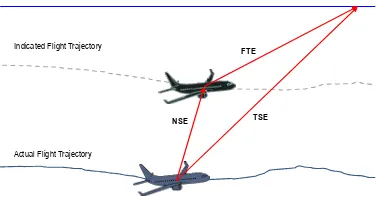
In aviation applications, accuracy is a measure of the difference between the estimated and the true or desired aircraft position under nominal fault-free conditions. It is normally expressed as 95% bounds on Horizontal and Vertical position errors [34]. In the avionics context, there are two distinguished types of accuracy that must be considered: the accuracy relative to the navigation system alone and the accuracy achieved by the combination of navigation and flight control systems. This second type of accuracy is called Total System Error (TSE) and is measured as deviation from the required flight trajectory. In large commercial aircraft and several military aircraft, the required flight trajectory and associated guidance information is computed by a Flight Management System (FMS) and constantly updated based on ATM and weather information. The navigation system estimates the aircraft state vector (i.e., position, velocity, attitude and associated rates), determines the deviation from the required flight trajectory and sends these information either to the cockpit displays or to an Automatic Flight Control System (AFCS). The error in the estimation of the aircraft’s position is referred to as Navigation System Error (NSE), which is the difference between the aircraft’s true position and its displayed position. The difference between the desired flight path and the displayed position of the aircraft is called Flight Technical Error (FTE) and accounts for aircraft dynamics, turbulence effects, human-machine interface, etc. As illustrated in Fig. 8, the TSE is obtained as the vector sum of the NSE and the FTE.

Required Flight Trajectory

Indicated Flight Trajectory

Actual Flight Trajectory

FTE

TSE NSE

Fig. 8. Navigation accuracy in aviation applications.

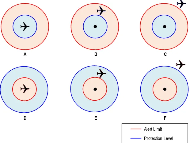
The integrity risk can be conveniently defined as the probability of providing a signal that is out of tolerance without warning the user in a given period of time. It is typically derived from the high-level Target Level of Safety (TLS) which is an index, generally determined through historic accident data, against which the calculated risk can be compared to judge whether the operation of the system is safe or not. The navigation integrity requirements in various flight phases/operational tasks have been specified by ICAO in terms of three key performance indicators: the probability of failure over time (or per single approach), the Time-To-Alert (TTA) and the Horizontal/Vertical Alert Limits. The TTA is the maximum allowable time elapsed from the onset of the system being out of tolerance until the equipment enunciates the alert. The alert limits represent the largest horizontal and vertical position errors allowable for safe operations. They are defined as follows [36]:

Horizontal Alert Limit (HAL): the HAL is the radius of a circle in the horizontal plane (the local plane tangent to the WGS-84 ellipsoid), with its center being at the true position, that describes the region that is required to contain the indicated horizontal position with the required probability for a particular navigation mode.

vertical position with the required probability for a particular navigation mode.

According to these definitions, in order to assess the navigation system integrity, the NSE must be determined first and checked against the Alert Limits (ALs) applicable to the current flight operational phase. However, since the NSE is not observable by the pilot or by the avionics on board the aircraft, another approach to evaluate the system integrity has to be adopted. The standard approach consists in estimating the worst-case NSE and confronting this value with the corresponding AL. These limits for NSE are known as Protection Levels (PLs) and represent high-confidence bounds for the NSE. Similarly to the positioning errors,

the PLs are stated in terms of Horizontal and Vertical components (HPL and VPL).

Table 7 lists the required level of accuracy, integrity, continuity and availability defined by ICAO for the different aircraft flight phases. Various applicable national and international standrads have been used in this compilation [37-41].

An additional performance indicator that is often used to characterise avionics GNSS receivers is the Time-To-First-Fix (TTFF). The TTFF accounts for the time elapsed from the GNSS receiver switch-on until the output of a navigation solution is provided to the user within the required performance boundaries (typically in terms of 2D/3D accuracy).

Table 7. Aviation GNSS Signal-in-Space Performance Requirements [37-41].

TYPE OF OPERATION

HOR./VERT. ACCURACY

(95%)

CONTINUITY AVAILABILITY INTEGRITY TTA HAL / VAL

En Route Oceanic 3700m/NA 1−10ିସ/hr to

1−10ି଼_/hr 0.99 to 0.99999 1−10ି଻/hr 5 min 7408m/NA

En Route

Continental 3700m/NA

1−10ିସ_{/hr to}

1−10ି଼_/hr 0.99 to 0.99999 1−10ି଻/hr 5 min 3704m/NA

En Route Terminal 740m/NA 1−10ିସ/hr to

1−10ି଼_/hr 0.99 to 0.99999 1−10ି଻/hr 15 s 1852m/NA

APV-I 16m/20 m 1−8 × 10ି଺/15 s 0.99 to 0.999 1−2 × 10ି଻/

App. 10 s 40m/50 m

APV-II 16m/8 m 1−8 × 10ି଺/15 s 0.99 to 0.999 1−2 × 10ି଻/

App. 6 s 40m/20m

Category I 16m/4m 1−8 × 10ି଺/15 s 0.99 to 0.99999 1−2 × 10ି଻/

App. 6 s 40m/10m

Category II 6.9m/2m 1−4 × 10ି଺/15 s 0.99 to 0.99999 1−10ିଽ/15 s 1 s 17.3m/5.3m

Category III 6.2 m/2 m

1−2 × 10ି଺_{/30 s} (lateral)

1−2 × 10ି଺_{/15 s} (vertical)

0.99 to 0.99999

1−10ିଽ_{/30 s} (lateral)

1−10ିଽ_{/15 s} (vertical)

1 s 15.5m/5.3m

The TTFF is commonly broken down into three more specific scenarios, as defined in the GPS equipment guide:

Cold Start: The receiver has no recent Position, Velocity and Time (PVT) data estimates and no valid almanac data. Therefore, it must systematically search for all possible satellites in the sky. After acquiring a satellite signal, the receiver can obtain the almanac data (approximate information relative to satellites), based on which the process of PVT estimation can start. For instance, in the case of GPS receivers, manufacturers typically claim the factory TTFF to be in the order of 15 minutes.

Warm Start: The receiver has estimates of the current time within 20 seconds, the current position within 100 km, and its velocity within 25 m/s, and it has valid almanac data. Therefore, it must acquire each satellite signal and obtain the satellite's detailed ephemeris data.

Hot Start: The receiver has valid PVT, almanac and ephemeris data, enabling a rapid acquisition of satellite signals. The time required by a receiver in this state to calculate a position fix is also called Time-to-Subsequent-Fix (TTSF). TTSF is particularly important in aviation applications due to frequent satellite data losses caused by high dynamics aircraft manoeuvres.

In aviation applications, GNSS alone does not guarantee the level of performance required in several flight phases and operational tasks. In particular, GNSS fails to deliver sufficient accuracy and integrity levels for mission-critical and safety-critical operations such as precision approach/auto-landing, avionics flight test and

flight inspection. Therefore, appropriate augmentation strategies must be implemented to accomplish these challenging tasks using GNSS as the primary source of navigation data.

3. GNSS Threats in Aviation

To meet the stringent SIS performance requirements of GNSS in the aviation context (Table 7), it is essential to detect, isolate and possibly predict GNSS data degradations or signal losses experienced by the aircraft during its mission. This concept applies both to civil and military (manned and unmanned) aircraft, although in different flight and operational tasks. Suitable mathematical models are therefore required to describe the main causes of GNSS signal outages/degradations including Doppler shift, interference/jamming, antenna obscuration, adverse satellite geometries, Carrier-to-Noise ratio (C/N0) reductions (fading), and

multipath (i.e., GNSS signals reflected by the Earth’s surface or the aircraft body).

3.1. Antenna Obscuration

Due to the manoeuvres of the aircraft, the wings, tail and fuselage will obscure some satellites during the flight. Fig. 9 shows the GNSS satellite obscuration algorithm.

different flight conditions. Besides the AOM, other factors influence the satellite visibility. In general, a satellite is geometrically visible to the GNSS receiver only if its elevation in the antenna frame is above the Earth horizon and the antenna elevation mask.

Fig. 9. GNSS satellite obscuration analysis.

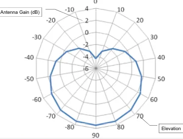
It should be noted that even high performance avionics GNSS antennae have gain patterns that are typically below -3dB at about 5 degrees elevation and, as a consequence, their performance become marginal below this limit (Fig. 10).

17-Feb-2012 39

© Roberto Sabatini, 2012 39

Antenna Gain (dB)

Elevation

Fig. 10. Avionics antenna gain pattern (L1 frequency).

In order to determine if a satellite is obscured, the LOS of the satellite with respect to the antenna phase centre has to be determined. To calculate the satellite azimuth and elevation with respect to the antenna transformation matrix between ECEF (Earth Centred Earth Fixed) and antenna frame must be applied. This is obtained from:

ܶா௔=ܶ௕௔∗ܶே௕∗ܶாே (52)

whereܶ_௕௔is the transformation matrix between the aircraft body frame and the antenna frame,ܶ_ே௕is the transformation matrix from ENU (East-North-Up) to body frame, andܶ_ாேis the ECEF to ENU transformation matrix.

3.2. GNSS Signal

The received signal strength is affected by a number of factors including transmitter and receiver characteristics, propagation losses and interferences. When necessary, the various factors contributing to the GNSS link budget and signal degradations due to interference can be combine. Multipath induced effects are considered separately. The ratio of total carrier power to noise

ܥ/ܰ଴ in dB-Hz is the most generic representation of received

signal strength. This is given by:

஼

ேబ=ܲ௧+ܩ௧+ܩ௥−ܮ௦−ܮ௔−ܮ௥−ߪ௠ −ܰ௙ (dB) (53)

where:

்ܲis the transmitted power level (dBw); ܩ௧is the satellite antenna gain (dBic);

ܩ௥is the receiver antenna gain toward the satellite; ܮ௦is the free space loss;

ܮ௔is the atmospheric attenuation (dry-air); ܮ௥is the rainfall attenuation;

ߪ௠ is the tropospheric fading; ܰ௙is the receiver noise figure.

As an example, Table 8 shows the expectedܥ/ܰ_଴for a receiver tracking a GPS satellite at zenith given a typical noise power density of -205 dBW-Hz [75]. The values ofܥ/ܰ_଴listed in Table 14 should be compared against the values required to acquire and track GPS signals. These thresholds are heavily dependent on receiver design and for most commercial GNSS receivers they are in the order of 28-33 dB-Hz for acquisition and 25-30 dB-Hz to maintain tracking lock [42, 43]. Current generation avionics GNSS receivers, which are designed to operate in high dynamics conditions, typically exhibit better C/N0thresholds [44, 45].

Table 8. Nominal receiver GPS signal power and received C/N0[43].

SV Block

IIR-M/IIF Frequency P or P(Y) C/A or L2C

Signal Power

L1 -161.5 dBW -158.5 dBW

L2 -161.5 dBW -160.0 dBW

C/ܰ_଴

L1 43.5 dB-Hz 46.5 dB-Hz

L2 43.5 dB-Hz 45 dB-Hz

Fig. 11. GPS satellite antenna coverage.

The difference in signal strength caused by this variation in path length is about 2.1 dB and the satellite antenna gain can be approximated by:

ܩ௧(݀ܤ)= 2.5413 ∗ݏ݅݊ܧ− 2.5413 (54)

where E is the elevation angle. Similarly, the avionics antenna gain pattern shown in Fig. 8 can be approximated by:

ܩ௥(݀ܤ)= 9.8756 ∗ݏ݅݊ܧ− 4.7567 (55)

3.3. Radiofrequency Interference

Intentional and unintentional RF interference (jamming) can result in degraded navigation accuracy or complete loss of the GNSS receiver tracking. Jammers can be classified into three broad categories: Narrowband Jammers (NBJ), Spread Spectrum Jammers (SSJ) and Wideband Gaussian Jammers (WGJ). In mission-essential and safety-critical GNSS applications, both intentional and unintentional jamming must be detected in the GNSS receiver and accounted for in the integrity augmentation architecture. Fortunately, a number of effective jamming detection and anti-jamming (filtering and suppression) techniques have been developed for military GNSS applications and some of them are now available for civil use as well. An overview of these techniques is presented in [49]. The J/S performance of a GNSS receiver at its tracking threshold can be evaluated by the following equation [1]:

ܬ/ܵ= 10݈݋݃ ܴܳ௖ቂ_ଵ଴బ.భ(಴ ಿ బ⁄ଵ )_{ಾ ಺ಿ}−_ଵ଴బ.భ(ଵ಴ ಿ బ⁄ )ቃ (56)

where Q is the processing gain adjustment factor (1 for NBJ, 1.5 for SSJ and 2 for WGJ),R_ୡis the code chipping rate (chips/sec) and(ܥ/ܰ_଴)_{ெ ூே}is the receiver tracking threshold (dB-Hz). Since the weak limit in an avionics receiver is the carrier tracking loop threshold (typically the PLL), this threshold is usually substituted for(ܥ/ܰ_଴)_{ெ ூே}. During some experimental flight test activities with unaided L1 C/A code avionics receivers, it was found that in all dynamics conditions explored and in the absence of jamming, a (ܥ ܰ⁄ ଴)of 25 dB-Hz was sufficient to keep tracking to the satellites

[44, 45]. Using this 25 dB-Hz tracking threshold, the ܬ/ܵ performance of the GPS receiver considering one of the satellites tracked (PRN-14) during the descent manoeuvre was calculated. The calculated C/ܰ_଴ for PRN-14 was approximately 37 dB-Hz. Using these ܬ/ܵvalues, the minimum range in metres from a jamming source can be calculated from:

ܴ௠ ௜௡=_ସగఒೕ൬10

ಶೃು೟ೕషುೝೕశಸೝೕషಽೝ೑

మబ ൰ (57)

whereܧܴܲ_௧௝is the effective radiated power of the jammer (dBw),

l_௝is the wavelength of jammer frequency (m),ܲ_௥௝is the received (incident) jamming power level at threshold = ܬ/ܵ+ܲ_௥௦(dBw),

ܲ௥௦is the minimum received (incident) signal power (dBw),ܩ௥௝is

the GNSS antenna gain toward jammer (dBic) and ܮ_௥௙is the jammer power attenuation due to receiver front-end filtering (dB).

3.4. Atmospheric Effects

GNSS signal frequencies (L-band) are sufficiently high to keep the ionospheric delay effects relatively small. On the other hand, they are not so high as to suffer severe propagation losses even in rainy conditions. However, the atmosphere causes small but non-negligible effects that must be taken into account. The major effects that the atmosphere has on GNSS signals include [42]:

 Ionospheric group delay/carrier phase advance;  Tropospheric group delay;

 Ionospheric scintillation;  Tropospheric attenuation;  Tropospheric scintillation.

The first two effects have a significant impact on GNSS data accuracy but do not directly affect the received signal strength (ܥ/ܰ_଴). Ionospheric scintillation is due to irregularities in the electron density of the Earth’s ionosphere (scale size from hundreds of meters to kilometres), producing a variety of local diffraction and refraction effects. These effects cause short-term signal fading, which can severely stress the tracking capabilities of a GNSS receiver. Signal enhancements can also occur for very short periods, but these are not really useful from the GNSS receiver perspective. Atmospheric scintillation effects are more significant in the equatorial and sub-equatorial regions and tend to be less of a factor at European and North-American latitudes.

Signal scintillation is created by fluctuations of the refractive index, which are caused by inhomogeneity in the medium mostly associated to solar activity. At the GNSS receiver location, the signal would exhibit rapid amplitude and phase fluctuations, as well as modifications to its time coherence properties. The most commonly used parameter characterizing the intensity fluctuations is the scintillation indexܵ_ସ, defined as [47]:

ܵସ=ට〈ூ మ_{〉ି〈ூ〉}మ

〈ூ〉మ (58)

where I is the intensity of the signal (proportional to the square of the signal amplitude) and〈 〉denotes averaging. The scintillation index S4 is related to the peak-to-peak fluctuations of the intensity. The exact relationship depends on the distribution of the intensity. According to [47], the intensity distribution is best described by the Nakagami distribution for a wide range of ܵ_ସ values. The Nakagami density function for the intensity of the signal is given by:

݌(ܫ) =_Γ௠_(௠೘₎ܫ௠ ିଵ_݁(ି௠ ூ) ₍₅₉₎

where the Nakagami “m-coefficient” is related to the scintillation index, S4 by:

݉ =_ௌరଵమ (60)

In formulating equation (61), the average intensity level ofܫis normalized to be 1. The calculation of the fraction of time that the signal is above or below a given threshold is greatly facilitated by the fact that the distribution function corresponding to the Nakagami density has a closed form expression which is given by:

ܲ(ܫ) = ∫_଴ூ݌(ݔ)݀ݔ= Γ(௠_Γ(,௠ ூ_௠) ) (61)

where Γ(݉,݉ ܫ) and Γ(݉)are the incomplete gamma function and gamma function, respectively. Using the above equation, it is possible to compute the fraction of time that the signal is above or below a given threshold during ionospheric events. For example, the fraction of time that the signal is more than݊dB below the mean is given byܲ(10ି௡/ଵ଴)and the fraction of time that the signal is more than݉ dB above the mean is given by 1 –ܲ(10௠/ଵ଴). Scintillation strength may, for convenience, be classified into three regimes: weak, moderate or strong [47]. The weak values correspond toܵ_ସ< 0.3, the moderate values from 0.3 to 0.6 and the strong case for ܵ_ସ > 0.6. The relationship between ܵ_ସ and the approximate peak-to-peak fluctuations ܲ_௙௟௨௖(dB) can be approximated by:

ܲ௙௟௨௖= 27.5 ×ܵସଵ.ଶ଺ (62)