Group based single image super resolution with online dictionary learning

R E S E A R C H

Open Access

Group-based single image

super-resolution with online dictionary

learning

Xuan Lu

, Dingwen Wang

, Wenxuan Shi

and Dexiang Deng

Abstract

Recently, sparse representation has been successfully used in single image super-resolution reconstruction. Unlike the traditional single image super-resolution methods such as image interpolation, the super-resolution with sparse representation reconstructs image with one or several constant dictionaries learned from external databases. However, the contents can vary significantly across different patches in a single image, and the fixed dictionaries cannot suit for every patch. This paper presents a novel approach for single image super-resolution based on sparse representation, which uses group as the basic unit, and trains dictionary with external database and the input low-resolution image itself for each group to ensure that the dictionary is suitable for the patches in the group. Simultaneous sparse coding algorithm is used to accelerate the processing and improve the result. Extensive

experiments on natural images show that our method achieves better results than some state-of-the-art algorithms in terms of both objective and human visual evaluations.

Keywords: Super-resolution, Sparse representation, Online dictionary learning, Non-local similarity

1 Introduction

Super-resolution (SR) is the method that uses one or several low-resolution (LR) images to reconstruct a high-resolution (HR) image. Denote the HR image asX, and the LR image asY, then the degradation ofXto form an LR image can be generally formulated by

Y=SHX+ν (1)

whereHrepresents the blurring process andSrepresents the down-sampling process.νis the additive noise. Super-resolution solves the inverse problem of the degradation while it remains extremely ill-posed, which means there are generally multiple solutions that can be degenerated to the same LR image.

The SR algorithms can be broadly classified into two classes: (i)the traditional method which focuses on the reconstruction with several LR images such as a short video;(ii)the example-based method which deals with a

*Correspondence: [email protected]

2International School of Software, Wuhan University, Wuhan 430072, People’s Republic of China

Full list of author information is available at the end of the article

single input LR image, which was called image halluci-nation by some articles [1–4]. In the traditional method, each LR image imposes a set of linear constraints to sta-bilize the solution of the unknown HR image. However, because the LR images lack high-frequency part, which was more sensitive to the human eyes, the traditional method cannot achieve a relatively high magnification fac-tor [1, 5]. In example-based method, the single image super-resolution remains much ill-posed because it has only one constraint. To cope with the ill-posed nature of image super-resolution, prior knowledge of natural images is usually employed for regularizing the solution to the following minimization problem:

X=argmin X

Y−SHX2₂+λJ(X) (2)

where J(X) is a regularization term specifying the prior knowledge of the HR image andλ is a scalar balancing between the quadratic fidelity term and the regularization term, such as the total variation (TV) regularization [6], edge smoothness [7], and gradient profile priors [8]. How-ever, these methods cannot recover fine details and have unnatural edges.

In the past several years, sparsity has been emerg-ing as one of the most significant properties of natural images [9]. The sparsity prior suggests that image patch can be well-represented as a sparse linear combination of elements from an appropriately chosen over-complete dictionary [10]. The sparsity-based regularization has achieved great success both qualitatively and quantita-tively. However, it still has a little jaggy and ringing artifact along the edges in the reconstructed image. One of the keys to improve the result is to find a more suitable dic-tionary. Different improvements were proposed [11–14], etc., and have gotten better results.

Another significant property exhibited in natural images is nonlocal self-similarity, which is based on an obser-vation that patches in a single natural image tend to redundantly recur many times inside the image, both within the same scale, as well as across different scales [15]. In recent works, the sparsity and the self-similarity of natural images are usually combined to achieve better performance [13, 16, 17].

Traditional algorithms which are mentioned above often use patch as the basic unit of sparse representation and train redundant dictionaries with fixed sample image sets. Zhang et al. [18] and Zhang et al. [19] exploit the concept of group-based sparse representation for general image inverse problem and develop an efficient and effec-tive algorithm for image restoration and image compres-sive sensing recovery. Inspired by these works, this paper uses group as the basic unit for image super-resolution. The main contribution of our proposed method is that we divide the input image into several groups to com-bine the sparsity and the self-similarity of natural images in a unified framework and improve the performance of the dictionary for each group with the novel online dic-tionary learning method, which is more suitable than the one trained with classic algorithms. Experiments show that the proposed algorithm outperforms many current state-of-the-art schemes.

The rest of the paper is organized as follows. Section 2 introduces the related works. Section 3 presents the proposed super-resolution method and gives its imple-mentation details. Section 4 shows various compari-son experiments. Section 5 gives the conclusions and discussions.

2 Background and preliminaries

2.1 Super-resolution via sparse representation

In this section, we review the work on the single image super-resolution via sparse representation which was first introduced by Yang et al. [20]. The basic unit of sparse rep-resentation for natural image is patch. Letx∈Rndenote the HR image patches of size√n×√n, andy∈Rmdenote the features of LR image patches. UseDh ∈ Rn×K and Dl ∈Rm×Kto denote the over-complete dictionaries ofK

atoms(K > n,K > m), which are trained from HR and the feature of LR patches from training images, respec-tively. And the patchesxcan be represented as a sparse linear combination with respect to Dh. Which means x

can be expressed as

x=Dhα (3)

where α is the sparse coefficient andα0 K. The

l0-norm counts the number of nonzero coefficients in vec-torα. The sparse representationαcan be estimated from its observationyby solving the followingl0-minimization problem below:

where parameterγbalances the fidelity term and the spar-sity of the solution andFis a feature extraction operator.

The l0-minimization is an NP-hard problem. Donoho [21] shows that it can be approximated byl1-minimization when αis sufficiently sparse. It can be expressed as fol-lows:

which is known in statistical literature as the lasso. Let Rk(·) denote the operator that extracts the patch xk from the image Xat the kth position, and its

trans-pose, denoted byRT_k(·), is the operator that puts back a patch into the kth position in the reconstructed image. The whole image X can be reconstructed by averaging all of the reconstructed patchesxk, which can be written

as [18]

where1nis a vector of sizenwith all its elements being 1

andNis the total amount of the patches.

The image patches can be overlapped to better suppress noise and block artifacts. Considering Eqs. (3) and (6), we define the following operator “◦” for convenience:

X=D◦Adef=

Considering Eq. (5), the super-resolution via sparse rep-resentation can be formulated as follows:

ˆ

WhileXˆ may not satisfy the reconstruction constraint (2) exactly, it should be projected onto the solution space of (1), computing

X=argmin X

SHX−Y2₂+λX− ˆX2₂ (9)

whereλbalances between the fidelity term and the regu-larization term.

2.2 Dictionary learning

The dictionary is usually learned from a set of training examplesX = {x1,x2,. . .,xt}, and it can be trained from

whereZis the set of sparse representations of the training setXand thel1-norm||Z||1is used for enforcing sparsity. Eq. (10) is not convex in bothDandZbut is convex in one of them when the other is fixed. So, it can be solved in an alternative manner overZandD.

In the previous subsection, we saw the successful image SR should guarantee the situation that each pair of HR and LR image patch has the same sparse representation with respect to the two dictionaries Dh and Dl, respectively.

Given a set of training sample pairsP = {Xh,Yl}, where

Xh = {x1,x2,. . .,xn} are the set of sampled HR image

patches andYl = {y1,y2,. . .,yn} are the corresponding

LR image patches. When the two dictionary learning pro-cesses combine and force the HR and LR representations to share the same code, they can be written as

min

where N andM are the dimensions of the HR and LR image patches in vector form. (11) can be rewritten as follows:

Thus, the strategy of single dictionary learning can be used for training the two dictionaries for SR purpose.

3 The proposed algorithm

The non-local similarity prior for natural images is based on an observation that patches in a single natural image tend to redundantly recur many times inside the image. On the other hand, natural images are believed to be

composed of simple local image structures, observed as singular primitives, such as lines and arcs [3]. These local singular primitives are invariant to scale changes. So, a patch has good matches around its original location in the lower scale image [22].

These researches show that an natural image can be divided into several groups. The patches in the same group have similar image structures and can be presented by a relatively compact dictionary, which is more suitable for the patches in the group than a redundant dictionary. We use group as the basic unit instead of patch to gain a better result at the same time.

We treat the input LR image as the image that contains some high-frequency contents but with unsatisfactory pixel resolution. So, it offers high-frequency information about the singular primitives and can be used in our group-based SR algorithm. LetXl ∈RK denote the input

LR image, whereKis the size of the whole image vector. We down-sampleXland then up-sample it using bi-cubic

interpolation by the same factor of sto obtain the low-frequency band imageYl ∈ RK. Then, we up-sampleXl

with bi-cubic interpolation by the factor ofsto obtain low-frequency bandYh ∈ Rs

2_K

of the unknown HR image Xh∈Rs

2_K

. Useyk_l,yk_h,xk_l, andxk_hto denote the vector rep-resentations of the image patch extracted fromYl,Yh,Xl,

andXhin thekth position, respectively.

Incorporating with the nonlocal similarity prior knowl-edge, for a patchyk_h, we search the similar patches around the corresponding place and make a group, which is denoted byGjyh, wherejis the group order, and the total

number of the group is denoted byL. Euclidean distance is selected as the similarity criterion between different patches. The number of the patches in the group isc, that is to say we choosec−1 patches that are most like the patchyk_hto make a group, and then delete them from the patch list. SoL= P_c, wherePis the total number of the patches and· is the ceiling function. The correspond-ing patches ofyi_h ∈ Gjyh(i = 1, 2,. . .,c)in image Yl can

also make a group, which is denoted byGjyl. The groupG

j yl

and its high-frequency versionGjxl provide the

informa-tion about the lost high-frequency band to the unknown imageXh.

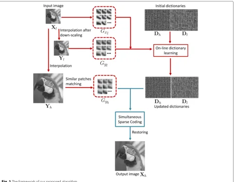
Figure 1 shows the framework of our proposed algo-rithm. We divide our strategy into two phases: the first is the online dictionary learning phase(marked as red lines) and the second is the simultaneous sparse coding phase (marked as blue lines). We show the details of the first phase in Section 3.1 and the second phase in Section 3.2.

3.1 Online dictionary learning phase

Fig. 1The framework of our proposed algorithm

potentially infinite data sets, adapt to dynamic training sets, and it is dramatically faster than traditional algo-rithms. Instead of using a fixed dictionary, we try to update dictionary during the image processing of each patch. The patches in groupGxjlcan be treated as the

cor-responding patches in groupGjylwith high frequency. And

the groupGjyl and the groupG

j

xl compose the training set.

To ensure that the HR dictionaryDhand the LR

dictio-naryDlhave the same sparse representation, we use the

method mentioned in Section 2.2 and transform the joint dictionary learning into a single one.

We subtract patches inGjyl from corresponding patches

inGjxl to obtain the high-frequency part as the HR

sam-ple group set, denoted by Gj_h. We extract the feature of patches inGjyl with the feature extraction operator F in

order to boost the prediction accuracy. In [2], high-pass filter was used as F to extract the edge information as the feature. In [24], a set of Gaussian derivative filters was used to extract the contours in the LR patches. In [25], the

wavelets of LR images were used to train dictionary. And in [10], the first- and second-order derivatives were used as the features:

f1=[−1, 0, 1] , f2=f1T

f3=[ 1, 0,−2, 0, 1] , f4=f3T

(14)

where the superscript “T” means transpose. In this paper, we use Eq. (14) asFdue to its simplicity and effectiveness. Instead of applying the four filters to the patches in groupGjyl directly, we apply these filters toYl to get the

four gradient maps and extract the four feature patches from the corresponding location. Then, we concatenate the vector representations of the four patches in the same location and form the LR sample vector group setGj_lfor dictionary training. Thus, we get the training group setGjc

for dictionary updating by rearranging the sample using the equation below:

Gjc=

₁

√

NG j h 1

√

MG j l

where N andM are the dimensions of the HR and LR image patches in vector form.

The formulation for the updating of the dictionary is shown below:

wherexj_i is the sample vector with index iin the group set Gjc and D0 is an initial dictionary which is learned using an external database. Thus, we have finished learn-ing dictionary Dj for the patches in the group with the indexj.

The basic unit of dictionary learning is still patch, but each dictionary is only updated by the patches in the corresponding groups. Different from the traditional dic-tionary learning method proposed by Yang et al. [10] that uses a single dictionary for the construction of all patches, this method also contained the information of all patches in the group in dictionary learning phase, which made the dictionary more suitable for the patches in the cor-responding group. Because the patches in the group are similar, the dictionary is relatively more compact than the initial one.

We randomly extracted 80,000 patches from 200 high-quality natural images from the Berkeley Segmentation Database [26]. With the same feature extractorF men-tioned above and the method introduced in Section 2.2, we can calculateD0.

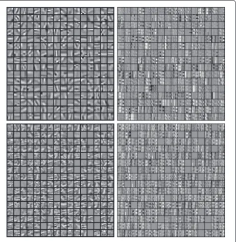
Figure 2 shows the HR dictionaryDh and the LR

dic-tionaryDllearned by our algorithm. The first row is the

primal dictionaries we used as the initial D0. The sec-ond row is the updated dictionaries during the process of the first group. It is obvious that some elements in the updated dictionaries are set to zero vectors, which reduce the size of the dictionaries. And the elements in the updated dictionaries are more specific than the initial ones.

3.2 Simultaneous sparse coding phase

The sparse coding phase attempts to magnify all of the patches in the input LR image Xl. After estimating the

low-frequency partYh of the final HR imageXh, we just

need to restore the high-frequency part and then add it toYh.

We apply simultaneous sparse coding to the sparse rep-resentation of each group. For traditional sparse coding,

Fig. 2Dictionaries used during the image process

similar patches in one group sometimes admit very dif-ferent estimates due to the potential instability of sparse decomposition, which can result in noticeable reconstruc-tion artifacts [27]. A simultaneous sparse coding algo-rithm makes approximation of several input signals at the same time using different linear combinations of the same elementary signals [28]. It solves the problem of the tra-ditional sparse coding by forcing similar patches to admit similar decomposition.

The joint sparse representationAjof the groupGjyhcan

be formulated as below:

iandαj_iis the sparse representation ofyi_hwith dictionary

Dj_l; where Aj = leading to a convex norm, while the latter actually counts the number of nonzero rows.

After obtaining Aj, the super-resolved patch xi_h in the groupGj_xhcan be written as

xi_h=Dj_hαj_i+yi_h (21)

With the extract and restore operator defined in (7), the whole imageXhcan be reconstructed by

Xh= L

j=1

Dj_h◦Aj+Yh (22)

Our method skips the back-project step mentioned in (9), because the sparsity prior is strong enough that we can already achieve good performance.

Algorithm 1 shows the complete process of our pro-posed method.

Algorithm 1The proposed algorithm

Input:Low-resolution imageXl, factors, initial dictionary D0, regularization parameter λ and γ, number of iterationsT.

1. Initialization:

(a) D←D0.

(b) Scale upXlwith factors using bi-cubic

interpolation to generateYh, down-sampleXl

and then interpolate it with the same factors to generateYl. Extract the feature ofYlusing (14).

(c) DivideYhintoP patches and then collect them

intoL groups according to the Euclidean distance.

2. forj=1,. . .,Ldo

(a) Collect the corresponding patches inXland

FYlof the patches in thej -th group ofYh, and

generate the training group setGjcusing (15).

(b) fori=1,. . .,cdo

Update the dictionaryDwith (17), and then get the high-resolution dictionaryDhand

low-resolution dictionaryDlusing (18). end for

(c) Compute sparse representationAjof patches in thej -th group ofYhin (19) withDlusing

S-OMP algorithm.

(d) Reconstruct the patches in thej -th group ofXh

withAjandDhusing (21).

end for

3. Put the patches in all groups back together to generate the output imageXh.

Output:High-resolution imageXh.

4 Experimental results

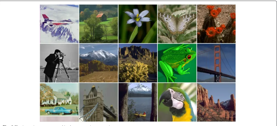
Figure 3 shows the 15 images that are used for compari-son. In our experiment, all the test images are applied a 7×7 Gaussian kernel of zero mean and standard devia-tion 1.0 and then down-sampled by a decimadevia-tion factor of 2 to produce the corresponding LR images.

We compare the proposed method with other four algo-rithms to illustrate the efficiency of our proposed method. The competed algorithms are bi-cubic interpolation [13, 15, 20]. Specifically, for methods based on fixed exter-nal dictionaries, we choose the work of Yang et al. [20] for comparison; for methods based on non-local similarity, we choose the work of Glasner et al. [15] for comparison; for methods that combine sparse representation and non-local similarity, we choose the representative work ASDS method [13] for comparison.

A frequently used criterion, peak signal-to-noise ratio (PSNR), is used for the image quality analysis. But it is sometimes not a reliable metric for evaluating the image quality. Therefore, the structural similarity (SSIM) index [29] and the feature similarity (FSIM) index [30] are also adopted for the objective evaluation. A higher PSNR value implies less distortion compared with the ground truth, and an SSIM value or an FSIM value much closer to 1 indicates the structure or the feature of the recon-structed image is more similar to the ground truth image, respectively.

For color image super-resolution, we only apply our algorithm on the illuminance component and use bi-cubic interpolation for the chromatic components, because human visual system is not sensitive to the chromatic components. In experiments, the value of PSNR, SSIM, and FSIM are all conducted on the illuminance compo-nent of the image.

4.1 Experimental configuration

We magnify the input LR image by factor of 2 and use 6×6 patches with an overlap of two pixels between adjacent patches, both for the HR imageYhandXhand LR image YlandXl; and we learned the dictionary of sizeK =128.

In the online dictionary learning phase, the sizeLof train-ing window is selected as 60, the numbercof best matched patches is 128, the sparsity regularization parameterλis 0.15, and the number T of iteration to train the dictio-nary is 32. In the simultaneous sparse coding phase, the parameterγ that balances the fidelity term and the reg-ularization term is 0.15, and the value of(p,q)is chosen as 1, 2.

Fig. 3The input images we used in the comparison experiments

The proposed algorithm is implemented by MATLAB R2011b usingSPAMS toolbox[31] for on-line dictionary learning and simultaneous sparse coding. The computer system used for simulation is Intel Core i7-4500U CPU at 1.80GHz with 8GB of RAM.

4.2 Noiseless experiment

4.2.1 Objective evaluations

For objective evaluations, Table 1 reports the results obtained by the proposed method and other super-resolution approaches. In this table, the proposed approach holds the best performance for most of the images. While for images such as cameraman or parrot, the proposed approach is not so good for the PSNR com-parisons. That is because the PSNR value just counts the error between pixel values in the two images while ignores the characteristics of human visual system. The training samples of the proposed method need to be normalized before online dictionary training according to the require-ment of the online training function. After the sparse approaching phase, the tonal range has a little bias in the histogram. This bias leads influences on the PSNR value.

The SSIM and FSIM value, which are more accurate than PSNR value to evaluate the image quality, simulate the characteristic of human visual system. The improve-ment of our results in SSIM and FSIM shows the structure and feature restoration are better than the other compet-ing methods.

4.2.2 Visual quality evaluations

For visual quality evaluations, Figs. 4, 5, 6, and 7 show the visual comparison of different approaches. In the figures, the results of bi-cubic interpolation are very blurry and

have staircase artifacts on the ramp. The results of Yang et al. [20] restore lots of details and sharp edges, while introducing noise and ringing artifacts. This method uses a fixed dictionary pair to try to restore the image but it cannot be suitable for different kind of structures. The results of Glasner et al. [15] seem too smooth to retain enough details. This method uses non-local similarity prior and extracts information only from the input image itself. It makes full use of the input image, but the high-frequency information in the input image is limited. The results of ASDS [13] are better than bi-cubic for less staircase artifacts and less blurry edges. The ASDS [13] algorithm uses several sub-dictionaries to match different kinds of micro-structures, but the sub-dictionaries cannot guarantee the coverage of all the micro-structures.

Our algorithm uses the dictionary trained from exter-nal databases to offer the missing high frequency and the input image itself to offer the ground truth information. The online learning updates the dictionary for each patch to combine the information of external databases and the ground truth. The updated dictionary is more suitable for the patch and avoids adding some artifacts to the restored image.

Table 1Comparisons of peak signal-to-noise ratio(PSNR) values, structural similarity (SSIM) values, and feature similarity (FSIM) values for 15 test images with different super-resolution approaches

Image Bi-cubic Yang et al. [20] Glasner et al. [15] ASDS [13] Proposed

Avion PSNR 27.01 29.13 28.48 31.62 30.92

SSIM 0.875 0.905 0.918 0.934 0.936

FSIM 0.863 0.902 0.907 0.930 0.936

Barnfall PSNR 29.16 30.14 29.88 30.76 30.51

SSIM 0.716 0.780 0.763 0.783 0.788

FSIM 0.825 0.895 0.862 0.893 0.899

Blueeye PSNR 33.39 34.00 35.28 36.37 36.75

SSIM 0.923 0.923 0.939 0.939 0.944

FSIM 0.946 0.957 0.960 0.962 0.968

Butterfly PSNR 28.51 30.13 29.85 32.22 31.51

SSIM 0.855 0.894 0.902 0.921 0.926

FSIM 0.909 0.930 0.935 0.947 0.950

Cactusflower PSNR 25.48 26.67 26.34 27.47 26.95

SSIM 0.658 0.763 0.728 0.749 0.764

FSIM 0.793 0.877 0.844 0.863 0.885

Cameraman PSNR 25.55 26.83 26.68 28.68 27.94

SSIM 0.827 0.862 0.869 0.892 0.899

FSIM 0.821 0.883 0.864 0.908 0.901

Colomtn PSNR 27.44 28.33 27.93 28.80 28.67

SSIM 0.685 0.747 0.729 0.749 0.757

FSIM 0.807 0.877 0.841 0.876 0.886

Desert PSNR 24.10 24.86 24.89 25.59 25.41

SSIM 0.677 0.757 0.737 0.780 0.786

FSIM 0.812 0.879 0.852 0.890 0.896

Frog PSNR 31.42 32.74 32.78 34.45 34.27

SSIM 0.895 0.920 0.927 0.937 0.944

FSIM 0.894 0.931 0.924 0.945 0.953

Goldgate PSNR 33.05 34.46 34.05 35.48 35.10

SSIM 0.873 0.899 0.907 0.908 0.912

FSIM 0.877 0.919 0.909 0.922 0.925

House PSNR 26.53 28.40 28.14 30.33 29.61

SSIM 0.817 0.863 0.865 0.892 0.894

FSIM 0.835 0.886 0.888 0.913 0.919

London PSNR 29.27 31.32 30.34 33.28 33.13

SSIM 0.850 0.894 0.894 0.915 0.919

FSIM 0.837 0.903 0.877 0.919 0.918

Lostlake PSNR 27.60 28.81 28.37 29.71 29.30

SSIM 0.749 0.806 0.795 0.819 0.824

FSIM 0.839 0.896 0.877 0.903 0.907

Parrot PSNR 28.93 31.21 30.19 34.05 32.92

SSIM 0.911 0.926 0.939 0.945 0.949

FSIM 0.917 0.948 0.938 0.959 0.957

Redrock PSNR 27.33 28.51 28.12 29.35 29.11

SSIM 0.773 0.834 0.820 0.847 0.851

FSIM 0.820 0.889 0.858 0.894 0.893

Fig. 4Comparison of SR results of blueeye image with magnification factor 2.Top row: bi-cubic, the method in [20], and the method in [15].

Bottom row: the method in [13], the proposed method, and the ground truth image

With the fixed size of the search window, many patches that are not so similar are also added into the training sam-ple set. This may mislead the dictionary updating, thus leads to a result that is not so fine. In addition, when the low-frequency part of the input image is too blurry, it also misleads the dictionary updating and produces blurry details.

In Fig. 4, the edges and the streaks of the petal of our method are clearer than that of Glasner et al. [15] and ASDS [13], while there is no additional noise and ringing artifact as which in the result of Yang et al. [20]. In Fig. 5, the fine lines in the wings of the butterfly are restored very well, and the round dot is not distorted when compared

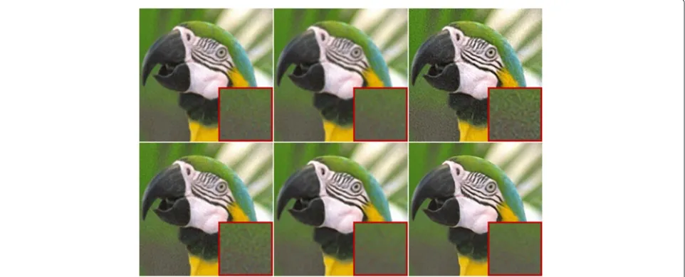
with the first three methods. Because the textures in the butterfly wings are repeated, which is convenient for us to collect much useful ground truth information about these details. The same reason is for the restoration of Fig. 6. The short stripes on the parrot’s face are separated in the results of bi-cubic, Yang et al. [20], ASDS [13], and our method, while the edges of other stripes in our result are sharper than that of bi-cubic and ASDS [13] and are more delicate than that of Yang et al. [20]. In Fig. 7, the details of the camera is restored better than the others, espe-cially the white fine line in the left bottom corner of the camera. Besides, it is obvious that the edges of the cam-eraman’s coat are sharper than others. These indicate that

Fig. 5Comparison of SR results of butterfly image with magnification factor 2.Top row: bi-cubic, the method in [20], and the method in [15].

Fig. 6Comparison of SR results of parrot image with magnification factor 2.Top row: bi-cubic, the method in [20], and the method in [15].

Bottom row: the method in [13], the proposed method, and the ground truth image

our algorithm can recover fine details and sharp edges at the same time.

4.3 Noisy experiment

In this subsection, we added Gaussian white noise with zero mean and standard deviation of 1, 3, and 5 to the LR image parrot and then compare the result of the five meth-ods. The objective evaluation is reported in Table 2 and the results of the LR image with noise levelσν = 5 with different approaches are shown in Fig. 8.

From the table and the figure, we can see that the results of Yang et al. [20] and Glasner et al. [15] enhanced the noise. The result of ASDS [13] performs the best on noise

suppressing, but this noise suppression also affects the image reconstruction and makes the result image more blurry than its result of noiseless image. The proposed method achieves a good result both on noise suppress-ing and image reconstruction. The proposed method is better than the other because the group-based dictionary learning phase gets a relatively compact and suitable dic-tionary for the patches in the group to be reconstructed. The sparse coding in each iteration in the online dic-tionary learning method helps suppress the noise in the training patches. Thus, the elements in the dictionary and the structures of the group have a correlation between them, while the elements are independent with the noise.

Fig. 7Comparison of SR results of cameraman image with magnification factor 2.Top row: bi-cubic, the method in [20], and the method in [15].

Table 2Comparisons of peak signal-to-noise ratio(PSNR) values, structural similarity (SSIM) values, and feature similarity (FSIM) values for image with different noise level with different super-resolution approaches

Noise level Bi-cubic Yang et al. [20] Glasner et al. [15] ASDS [13] Proposed

σν=0 PSNR 28.93 31.21 30.19 34.05 32.92

SSIM 0.911 0.926 0.939 0.945 0.949

FSIM 0.917 0.948 0.938 0.959 0.957

σν=1 PSNR 28.92 31.13 30.17 31.34 32.92

SSIM 0.910 0.918 0.935 0.908 0.947

FSIM 0.917 0.945 0.937 0.934 0.956

σν=3 PSNR 28.83 30.49 29.94 31.24 32.67

SSIM 0.897 0.863 0.908 0.907 0.934

FSIM 0.913 0.918 0.925 0.936 0.952

σν=5 PSNR 28.66 29.41 29.46 30.96 32.18

SSIM 0.875 0.779 0.860 0.896 0.911

FSIM 0.904 0.872 0.901 0.934 0.941

The data in italics indicates the best PSNR/SSIM/FSIM result

Combined with the simultaneous sparse coding phase, the noise is suppressed and the structure and the details are retained.

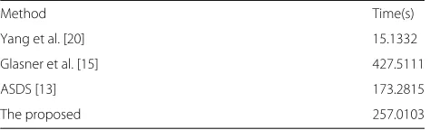
4.4 Time comparisons

In this subsection, we compare the running time of the four methods. We have ignored the time of training dic-tionaries for Yang et al. [20] and ASDS [13] and the time of training initial dictionaries for the proposed method.

We count the mean times for all configuration of the 15 images experiments, and Table 3 shows the running time of the compared methods. From the table, we can see that the shortest running time is that of Yang et al. [20]. The running time of Glasner et al. [15], ASDS [13], and the proposed method is comparable. Although we use

online dictionary learning algorithm during the process-ing which costs a large amount of time, we use group as the basic unit to reduce the dictionary learning times, and the simultaneous sparse coding algorithm also accelerates the processing.

5 Conclusions

This paper describes a novel method of group-based single image super-resolution. With the property of non-local self-similarity, we divide the input image into several groups. Combining with the information from external databases, we train suitable dictionaries for each group using online dictionary learning method. Simultaneous sparse coding algorithm is used to accelerate the pro-cessing and improve the result. Experiments show that

Table 3Time comparisons of different approaches

Method Time(s)

Yang et al. [20] 15.1332

Glasner et al. [15] 427.5111

ASDS [13] 173.2815

The proposed 257.0103

the proposed method can restore sharp edges and fine details and achieve good result on noise suppressing. The running time is comparable with other state-of-the-art algorithms.

In this paper, we just use the traditional Euclidean dis-tance for the searching of the similar patches to make a group. For further research, we will focus on developing a evaluation that directly measure the probability between two patches that belong to the same group to improve the performance of the proposed method.

Acknowledgements

This work was supported by National Natural Science Foundation of China (Grant No. 61501334).

Availability of data and materials

The images supporting the conclusions of this article are available in the “Test Images of Computer Vision Group”, All of the images are Copyright free. http://decsai.ugr.es/cvg/index2.php.

Authors’ contributions

XL and DW designed and carried out the experiments. XL and DD analyzed the experimental results. XL wrote the manuscript. WS and DD gave the critical revision and final approval. All authors read and approved the final manuscript.

Competing interests

The authors declare that they have no competing interests.

Author details

1_{School of Electronics and Information, Wuhan University, Wuhan 430072,}

People’s Republic of China.2International School of Software, Wuhan University, Wuhan 430072, People’s Republic of China.3_{School of Remote} Sensing and Information Engineering, Wuhan University, Wuhan 430072, People’s Republic of China.

Received: 20 February 2016 Accepted: 14 July 2016

References

1. B Simon, K Takeo, Limits on super-resolution and how to break them. IEEE Trans. Pattern Anal. Mach. Intell.24(9), 1167–1183 (2002)

2. TF Willian, CP Egon, Learning low-level vision. Int. J. Comput. Vis.40(1), 25–47 (2000)

3. TF Willian, RJ Thouis, CP Egon, Example-based super-resolution. IEEE Comput. Graph. Appl.22(2), 56–65 (2002)

4. S Jian, Z Jieie, FT Marshall, inIEEE Conference on Computer Vision and Pattern Recognition. Context-constrained hallucination for image super-resolution (IEEE, San Francisco, CA, USA, 2010), pp. 231–238 5. L Zhouchen, S Heung-Yeung, Fundamental limits of reconstruction-base

superresolution algorithms under local translation. IEEE Trans. Pattern Anal. Mach. Intell.26(1), 83–97 (2004)

6. M Antonio, JO Stanley, Image super-resolution by tv-regularization and Bregman iteration. J. Sci. Comput.37(3), 367–382 (2008)

7. D Shengyang, H Mei, X Wei, W Ying, G Yihong, KK Aggelos, Softcuts: a soft edge smoothness prior for color image super-resolution. IEEE Trans. Image Process.18(5), 969–981 (2009)

8. S Jian, S Jian, X Zongben, S Heung-Yeung, inIEEE Conference on Computer Vision and Pattern Recognition. Image super-resolution using gradient profile prior (IEEE, Anchorage, Alaska, USA, 2008), pp. 24–26 9. MB Alfred, LD David, E Michael, From sparse solutions of systems of

equations to sparse modeling of signals and images. Siam Rev.51(1), 34–81 (2009)

10. Y Jianchao, W John, H Thomas, M Yi, Image super-resolution via sparse representation. IEEE Trans. Image Process.19(11), 2861–2873 (2010) 11. Y Jianchao, W Zhaowen, L Zhe, C Scott, H Thomas, Coupled dictionary

training for image super-resolution. IEEE Trans. Image Process.21(8), 3467–3478 (2012)

12. Z Jian, Z Chen, X Ruiqin, M Siwei, Z Debin, inIEEE International Symposium on Circuits and Systems. Image super-resolution via dual-dictionary learning and sparse representation (IEEE, COEX, Seoul, Korea, 2012), pp. 1688–1691

13. D Weisheng, Z Lei, S Guangming, W Xiaolin, Image deblurring and super-resolution by adaptive sparse domain selection and adaptive regularization. IEEE Trans. Image Process.20(7), 1838–1857 (2011) 14. G Xinbo, Z Kaibing, T Dacheng, L Xuelong, Joint learning for single-image

super-resolution via a coupled constraint. IEEE Trans. Image Process.

21(2), 469–480 (2012)

15. G Daniel, B Shai, I Michal, inProceedings of the 12th International Conference on Computer Vision: 29 September-2 October 2009. Super-resolution from a single image (IEEE, Kyoto, 2009), pp. 349–356 16. GN Aneesh, SN Madhu, R Jeny, Single image super resolution from

compressive samples using two level sparsity based reconstruction. Procedia Comput. Sci.46, 1643–1652 (2015)

17. D Weisheng, S Guangming, Z Lei, W Xiaolin, Super-resolution with nonlocal regularized sparse representation. Proc. SPIE Visual Commun. Image Process.7744, 77440–17744010 (2010)

18. Z Jian, Z Debin, G Wen, Group-based sparse representation for image restoration. IEEE Trans. Image Process.23(8), 3336–3351 (2014) 19. Z Jian, Z Debin, J Feng, G Wen, inData Compression Conference (DCC),

2013. Structural group sparse representation for image compressive sensing recovery (IEEE, Snowbird, UT, 2013), pp. 331–340

20. Y Jianchao, W John, H Thomas, M Yi, inIEEE Conference on Computer Vision and Pattern Recognition. Image super-resolution as sparse representation of raw image patches (IEEE, Anchorage, AK, USA, 2008), pp. 1–8 21. LD David, For most large underdetermined systems of equations, the

minimal l1-norm near-solution approximates the sparsest near-solution. Commun. Pure Appl. Math.59(7), 907–934 (2006)

22. Y Jianchao, L Zhe, C Scott, inIEEE Conference on Computer Vision and Pattern Recognition. Fast image super-resolution based on in-place example regression (IEEE, Portland, OR, USA, 2013), pp. 1059–1066 23. M Julien, B Francis, P Jean, S Guillermo, Online learning for matrix

factorization and sparse coding. J. Mach. Learn. Res.11, 19–60 (2010) 24. S Jian, Z Nan-Ning, T Hai, S Heung-Yeung, inIEEE Conference on Computer

Vision and Pattern Recognition. Image hallucination with primal sketch priors, (Madison, Wisconsin, USA, 2003), pp. 729–736

25. A Na, P Jinye, Z Xuan, F Xiaoyi, Sisr via trained double sparsity dictionaries. Multimedia Tools Appl.74(6), 1997–2007 (2013)

26. The Berkeley Segmentation Dataset and Benchmark. http://www.eecs. berkeley.edu/Research/Projects/CS/vision/grouping/segbench. Accessed June 2007

27. M Julien, B Francis, P Jean, S Guillermo, Z Andrew, inIEEE International Conference on Computer Vision. Non-local sparse models for image restoration (IEEE, Kyoto, Japan, 2009), pp. 2272–2279

28. AT Joel, CG Anna, JS Martin, Algorithms for simultaneous sparse approximation. part i: Greedy pursuit. Signal Process.86(3), 572–588 (2006)

29. W Zhou, CB Alan, RS Hamid, PS Eero, Image quality assessment: from error visibility to structural similarity. IEEE Trans. Image Process.13(4), 600–612 (2004)

30. Z Lin, Z Lei, M Xuanqin, Fsim: a feature similarity index for image quality assessment. IEEE Trans. Image Process.20(8), 2378–2386 (2011) 31. SPArse Modeling Software. http://spams-devel.gforge.inria.fr/downloads.