Experimenting with career concerns

(1)

Manuscript version: Author’s Accepted Manuscript

The version presented in WRAP is the author’s accepted manuscript and may differ from the published version or Version of Record.

Persistent WRAP URL:

http://wrap.warwick.ac.uk/117651 How to cite:

Please refer to published version for the most recent bibliographic citation information. If a published version is known of, the repository item page linked to above, will contain details on accessing it.

Copyright and reuse:

The Warwick Research Archive Portal (WRAP) makes this work by researchers of the University of Warwick available open access under the following conditions.

practicable the material made available in WRAP has been checked for eligibility before being made available.

Copies of full items can be used for personal research or study, educational, or not-for-profit purposes without prior permission or charge. Provided that the authors, title and full

bibliographic details are credited, a hyperlink and/or URL is given for the original metadata page and the content is not changed in any way.

Publisher’s statement:

Please refer to the repository item page, publisher’s statement section, for further information.

(2)

Experimenting with Career Concerns

∗

Marina Halac

†

Ilan Kremer

‡

July 18, 2018

Abstract

A manager who learns privately about a project over time may want to delay quitting it if recognizing failure/lack of success hurts his reputation. In the banking industry, managers may want to roll over bad loans. How do distortions depend on expected project quality? What are the effects of releasing public information about quality? A key feature of banks is that they learn about project quality from bad news, i.e. a default. We show that in such an environment, distortions tend to increase with expected quality and imperfect information about quality. Results differ if managers instead learn from good news.

∗_{We thank Simon Board, Patrick Bolton, Tri Vi Dang, Peter DeMarzo, Wouter Dessein, Marco Di Maggio,}

Brett Green, Zhiguo He, Matt Jackson, Navin Kartik, Avi Lichtig, Qingmin Liu, Matteo Maggiori, George Mailath, Konrad Mierendorff, Pauli Murto, Andrea Prat, Canice Prendergast, Andy Skrzypacz, Lars Stole, Phillip Strack, various seminar and conference audiences, and two anonymous referees for helpful comments. We also thank Johannes H¨orner, Paul Milgrom, Dan Quint, and Curt Taylor for valuable discussions of the paper. Yifeng Guo provided excellent research assistance.

†_{Yale University and CEPR. Email:} _{[email protected]}_.

(3)

When a manager learns privately about a project over time, the market cannot assess the full consequences of his behavior, and the manager may want to take suboptimal actions that make a better impression (e.g., Prendergast and Stole, 1996). In particular, a manager may want to delay quitting a project if recognizing failure/lack of success hurts his reputation. How do distortions depend on expected project quality? Are managers more likely to keep bad ventures during good times, when expected quality is higher? What are the effects of releasing public information about project quality?

Following the financial crises over the last 30 years, there has been a growing concern about banks’ behavior during boom times. It is by now well documented that financial crises have often been preceded by credit booms (e.g., Schularick and Taylor, 2012). One reason for unhealthy credit growth is that banks may lower their standards and lend to low-quality borrowers who are unlikely to repay in a downturn. But there is also another reason for concern: during good times, banks may prefer not to force bankruptcy and instead roll over bad debt, providing life support to projects that, from an economic point of view, should be terminated. This practice of rolling over bad loans indeed appears to have played an important role in many crises, including Japan’s in the early 90s,1 _{and is at the center of current concerns}

about China. According toThe Wall Street Journal(2013), “the reason China’s bad-debt levels are so low boils down to the tendency of the country’s banks to routinely extend or restructure loans to borrowers, or sell them, rather than admit they have gone bad and record a loss in their accounts.”2 _{These problems have prompted efforts in several countries to generate more}

information about banks’ assets, for example by adopting stress testing and requiring public disclosure of test results (e.g., Hirtle and Lehnert,2014).

In a seminal paper,Rajan(1994) finds evidence of banks rolling over bad debt in good times and proposes a simple static model of career concerns to explain bank managers’ incentives. The pattern of distortions in a richer setting, however, is not obvious. On the one hand, as Rajan (1994) points out, a bank’s reputation cost of recognizing bad debt is larger in good times, when the perceived quality of loans is higher, compared to bad times. On the other hand, the fraction of problematic loans is also smaller in good times, so the potential for distortions is lower. The effects of releasing information are alsoa prioriunclear: perfect public

1_{Sekine, Kobayashi and Saita} ₍₂₀₀₃_{) and} _{Peek and Rosengren} ₍₂₀₀₅_{) find evidence that banks in Japan} continued to lend to severely impaired borrowers in order to avoid realizing losses on their own balance sheets. See alsoCaballero, Hoshi and Kashyap(2008).

2_{The article shows that while China had a low nonperforming loan ratio in 2012 compared to other countries,} its nonperforming loans in billions of yuan were steadily increasing over 2011-2013. According toThe Economist

(4)

information about loan quality would eliminate any scope for distortions, but is imperfect information also beneficial? We develop a dynamic model of career concerns to examine the pattern of distortions and the value of information. Our dynamic framework reveals that the nature of information managers receive over time is important for understanding these issues. Specifically, a key factor in the banking industry is that managers learn about project quality from the arrival of “bad news”: the structure of debt contracts implies that banks get more information when a borrower is in distress and defaults than when the loan is paid in full.3 _{This contrasts, for example, with the case of an entrepreneur investing in a technological}

innovation, who learns from the good news that arrive when a breakthrough occurs.

In our model, a manager decides at each time whether to continue to invest in a given project or abandon it. The quality of the project can be either good or bad and is initially unknown to all parties. The manager cares not only about the payoffs from the project but also about the market’s perception of the project’s quality. The market’s perception is based on the publicly observable actions of the manager, namely whether he continues or not with the project. The manager learns about the project’s quality from privately observed lump sum payoffs that arrive at random times. We contrast two scenarios. Our main focus is on a bad news setting, where the manager learns from the arrival of a negative payoff that indicates that the project is bad (and thus expected to generate losses). Here “no news is good news”: over time, in the absence of a negative payoff, the manager becomes more optimistic about the quality of the project. As a benchmark we examine a good news setting, where the manager learns from the arrival of a positive payoff that indicates that the project is good (and thus expected to generate positive profits). In this case “no news is bad news”: the manager becomes more pessimistic as time passes and a positive payoff does not arrive.

We characterize the manager’s decision of whether and when to abandon the project, and how in turn the market updates its belief over time. In both of the information environments we study, we solve for the (essentially) unique equilibrium in closed form.4 _{We show that the}

manager’s career concern generates an inefficiency: the manager runs the project for too long relative to the first-best solution that maximizes the expected payoff from the project. In the setting in which learning about project quality is through the arrival of bad news, the manager follows a pure strategy: he abandons the project if and only if bad news arrive before a given datet∗_{. As the manager continues with the project before reaching}_t∗_{, the market’s belief that}

the project is good increases; beyond t∗_{, the reputation cost of quitting is so large that the}

manager prefers to continue with the project even when he knows it will generate losses. In

3_As _Townsend₍₁₉₇₉_{) and} _{Dang, Gorton and Holmstr¨om}₍_2015a_,_b_{) argue, debt contracts enable banks to} minimize the cost of monitoring by not acquiring information when there is no default.

(5)

the good news setting, instead, the manager uses a mixed strategy: as time passes without the arrival of good news and the manager becomes more pessimistic, he follows a random quitting policy, abandoning the project at a later time than the efficient (pure) stopping time. In both settings, distortions are increasing, and welfare is decreasing, in the importance of career concerns.

Our characterization yields two main results. First, we show that in the bad news setting, distortions are more pronounced when the expected quality of the project is relatively higher.5

Distortions in this setting take the form of the manager keeping the project after learning that it is bad, namely when bad news first arrive after time t∗. When the prior probability of a good project increases,t∗ decreases, meaning that the manager is even less likely to quit following bad news. We show that this higher tendency not to terminate bad projects more than compensates for the fact that a bad project is less likely, so the overall distortion increases when expected quality rises. This result contrasts with what we find in the good news setting. Distortions in that setting take the form of the manager keeping the project after enough time has passed and good news have not arrived, namely after he has reached the efficient stopping time without good news. When the prior probability of a good project increases, the manager is more likely to keep the project for a longer period of time; however, the efficient stopping time also increases, so good news are more likely to arrive prior to this time. We show that as a consequence, distortions can decrease with expected quality in the good news setting.

Our second main result concerns the effects of information. Suppose that it is possible to release a public signal at the beginning of time that makes the market and manager’s common prior on the project more precise. This signal allows for a better assessment of the quality of projects and thus always weakly increases first-best welfare. The effects on equilibrium welfare depend on how the signal affects distortions. Naturally, if the signal is perfect, it eliminates distortions, as the manager’s actions cannot influence the market’s belief when the project’s quality is known. We show however that in the bad news setting, the effects of information are non-monotonic: a sufficiently imperfect signal increases the distortion relative to first best and reduces welfare. Intuitively, a high signal realization increases the prior that the project is good and (by the result described above) increases the distortion relative to first best, whereas a low signal realization reduces the prior and thus reduces the distortion. We find that distortions are convex in the prior, and therefore the former effect dominates when the signal is sufficiently imperfect.6 _{Moreover, such a signal leaves first-best welfare unchanged,}

5_{We describe here our results for “intermediate” parameter values, under which the equilibrium features} an interior timet∗

∈(0,_∞). SeeSection 2for details.

(6)

so the increase in distortions causes overall welfare to go down. These results are in contrast with what we find in the good news setting: releasing a public signal about project quality at the beginning of time always increases welfare when the manager learns through good news.

Our analysis highlights the role of dynamic aspects in shaping the effects of career concerns and yields different predictions for different applications. Returning to the banking industry, we find that the nature of learning in this industry explains why banks generate distortions especially in good times, and moreover implies that releasing information about the quality of credit may not help but rather exacerbate distortions. An implication of our analysis is the need for policy that pays close attention to refinancing during boom periods as well as the effects of supervisory tests and disclosure requirements. Simple restrictions are unlikely to do the job; in fact, policy aimed at reducing bad debt must deal with the problem that banks are often “creative” when it comes to refinancing loans. For the case of China, The Wall Street Journal (2013) explains that “banks need a reason to justify rolling over a loan, particularly if a company can’t repay it. (...) When they do roll over loans, Chinese banks sometimes do it in creative ways. To skirt restrictions on rolling over loans, banks cooperate with informal lenders that provide bank customers with short-term loans with high interest rates. That borrowing is used to repay a bank loan on the understanding that the bank will issue a new loan two or three weeks later. Such behavior can, in some instances, lead to bigger corporate-debt burdens.”

Related literature. There is a large literature on career concerns. One strand of this literature, in the tradition ofHolmstr¨om (1999), studies moral hazard models in which career concerns are beneficial because they incentivize agents to exert effort. These are models where outcomes are observable but actions are not.7 _{Our paper fits into a different strand of this}

literature, in which career concerns are detrimental because they lead to perverse incentives. Here actions are observable but outcomes are not. A seminal paper is Prendergast and Stole

(1996), where an agent has private information about his ability to understand the state of the world and distorts his decisions over time to look as a fast learner. Related issues are studied inScharfstein and Stein (1990), Zwiebel (1995),Majumdar and Mukand (2004), Prat (2005),

Ottaviani and Sørensen(2006), and Aghion and Jackson(2016).8

Within finance, as mentioned above,Rajan(1994) studies a static model in which a career-concerned bank manager chooses whether to implement a liberal credit policy that makes a bad loan less visible. Makarov and Plantin(2015) show that a fund manager will want to take

7_{Bonatti and H¨orner}₍₂₀₁₅_{) consider a version of}_Holmstr¨om_{’s model with exponential learning.}

(7)

on hidden tail risk when concerned with investors’ perception of his ability to generate excess returns above a fair compensation for risk. A number of papers point out that managers with stock-based compensation may still have a conflict of interest with shareholders (see Bond, Edmans and Goldstein, 2012, Section 3 for a survey), although only a few study how this conflict can result in actions directly aimed at concealing or revealing information. Among these, Benmelech, Kandel and Veronesi (2010) show that to prevent stock price reductions, managers may use suboptimal investment policies that conceal slowdowns in the firm’s growth opportunities. Frenkel (2017) examines a dynamic bargaining model in which managers with stock-sensitive compensation distort the price and timing of over-the-counter asset sales.

Our model is more closely related to those in Grenadier, Malenko and Strebulaev (2014),

Bobtcheff and Levy (2017), and Thomas (2016), all of which consider environments with exponential learning.9 _{Grenadier et al.}₍₂₀₁₄_{) examine an experimentation setting with public}

good news in which an agent is privately informed about his value of project success. The agent delays stopping because, unlike in our model, stopping at a later time signals a higher type.10 _{Bobtcheff and Levy} ₍₂₀₁₇_{) analyze a real option model in which a cash-constrained}

agent may learn bad news prior to investing. The agent wants to convey that his privately known learning intensity is high to raise capital more cheaply, and this can lead to hurried or delayed investment. Thomas (2016) studies a career concerns problem similar to ours, in which an agent learns about a project over time and can choose to abandon it. In her model, however, successes and failures are public, the agent learns privately from partially informative signals without cash-flow consequences, and the agent receives a reputation payoff only when the project succeeds, fails, or is terminated. The focus is also different: Thomas examines the conditions under which efficiency obtains,11 _{whereas we study the pattern of distortions,}

specifically how distortions vary with expected project quality and information about quality. More broadly, our paper is related to a sizable literature on exponential-bandit learning, including the seminal work of Keller, Rady and Cripps(2005). Most of this literature studies learning through good news, but there are exceptions: in addition to the papers described above,Bonatti and H¨orner(2017) andKeller and Rady(2015) consider bad news learning, and

Che and H¨orner (2017),Frick and Ishii (2015), andKhromenkova (2015) compare good news

9_{Also related is} _Bar-Isaac ₍₂₀₀₃_{), where a monopolist sells units over time whose (observable) success} depends on the monopolist’s fixed quality. While there is no private learning, the monopolist may have initial superior information about his quality, and thus his decision to continue trading can serve as a signal.

10_{The paper shows that if a public shock forces some agents to stop, then others will blend with the crowd} and stop strategically at the same time. Related papers of strategic delay include Acharya, DeMarzo and Kremer(2011) andGrenadier and Malenko(2011). See alsoGratton, Holden and Kolotilin(2017).

(8)

and bad news learning in various contexts.12 _{Some articles study how information disclosure}

affects experimentation, although this information is typically about outcomes rather than the underlying state as in our paper. In a career concerns setting, seePei (2015) and, outside the exponential bandit framework,H¨orner and Lambert (2016).13

1 Model

Players and actions. Consider an agent and a market. Time is continuous, the horizon is infinite, and the discount rate is r > 0. The agent has a project and, at each time t ≥ 0, decides whether to continue working on the project or to stop. To simplify the exposition, we assume that stopping is irreversible.14

The quality of the agent’s project is either “good” or “bad”, a fully persistent state. Work-ing on the project yields the agent an instantaneous payoffx_∈R, capturing the instantaneous

cost of working and any deterministic flow revenue from the project (so thatxmay be positive or negative). In addition, if the agent works at timetand the project is bad, the agent receives a lump-sum payoff of −1 at t with instantaneous probability λB ≥ 0; if the agent works at

time t and the project is good, he receives a lump-sum payoff of 1 at t with instantaneous probability λG ≥ 0. This structure allows us to embed both a bad news setting and a good

news setting, as we describe below. We assume x+λG>0> x−λB, i.e. the expected payoff

from the project is positive if the project is known to be good and negative if it is known to be bad. The payoff from not working is normalized to zero.

Information. The quality of the agent’s project is initially unknown to both the agent and the market. We denote byµ_t the agent’s time-t belief that the project is good. The exogenous prior belief isµ₀ _∈(0,1), commonly known also to the market.

The market only observes the agent’s decision at each point of whether to continue or to stop working on the project; the realized payoffs from the project are nonverifiable and privately observed by the agent. Hence, at any time t > 0, the market’s belief about the project may differ from the agent’s belief, as it is updated based on the agent’s actions only. We denote by _bµ_t the market’s time-t belief that the project is good.

12_{See also}_{Abreu, Milgrom and Pearce}₍₁₉₉₁_{) and}_{Board and Meyer-ter-Vehn}₍₂₀₁₂_).

13_{Rosenberg, Solan and Vieille} ₍₂₀₀₇_{) study a model of social experimentation in which agents observe} their opponents’ actions but not their opponents’ payoffs, and the decision to abandon the risky project is irreversible. Quah and Strulovici (2009) examine the comparative statics of optimal stopping time problems in a general framework.

(9)

Since the quality of the project is uncertain and may be learnt when the agent works, we say that the agent “experiments” when he runs the project.

Bad news versus good news. We focus on a setting in which the agent learns about project quality through bad news events: λB > λG = 0, and, to avoid trivialities, we then

assumex > 0 (where, as noted, x−λB <0). The agent therefore earns small profits so long

as he does not experience a “failure,” namely a lump-sum payoff of−1. Learning in this bad news environment takes the form of slow improvement in the agent’s beliefµt until the agent

fails and learns that the project is bad. We contrast this setting with one in which learning occurs through good news events: λG > λB = 0, and (again to avoid trivialities) we then

assume x < 0 (where, as noted, x+λG > 0). Here the agent incurs small losses so long as

he does not experience a “success,” namely a lump-sum payoff of 1. Learning in this good news environment takes the form of slow deterioration of the agent’s belief µ_t until the agent succeeds and learns that the project is good.

Payoffs. The agent cares not only about the payoff from the project but also about how his project is perceived by the market. The quality of the project reflects the agent’s skills and potential to select and successfully work on new projects. A career-concerned agent will therefore want the market to believe that his project is good rather than bad.

Following Rajan (1994) and Prendergast and Stole (1996), we take the agent’s payoff at each timet _≥0 to be a weighted sum of the project payoff and the reputation payoff the agent receives from the market’s perception, _bµ_tR, where R ≥ 0. Specifically, if the agent works on the project only until time τ, his time-0 payoff is

Z ∞

0

e−rt{[x+µ₀λG−(1−µ0)λB]1t<τ +µbtR}dt, (1)

where 1t<τ is an indicator function taking the value 1 if t < τ and zero otherwise. This

formulation captures, in a simple reduced form, any benefits the agent may enjoy from having a high reputation, such as outside options that increase the agent’s wage or the possibility of working on additional projects.15 _{For example, like money managers in} _{Dasgupta and} Piacentino (2015), banks differ in their ability to pick good investments, and they benefit from having a reputation for being good pickers as this allows them to attract more capital. Entrepreneurs and venture capital funds have similar career concerns, especially since they must repeatedly raise money from investors, as emphasized byBaker(2000).16

(10)

We will refer to expression (1) when R = 0 as social welfare. Controlling for project quality, society does not benefit from the agent having a high reputation, and the efficient allocation of productive resources is the one that maximizes the profits from the project. For example, if the project is a publicly traded company, then welfare corresponds to the utility of the investors.

To focus the exposition, throughout the paper we assume parameters are such that some experimentation is socially efficient, even if the agent is myopic:

Assumption 1. Some experimentation is always efficient: x+µ0λG−(1−µ0)λB >0.

Strategies and equilibrium. The agent’s history at time t, ht_{, consists of his private}

history of payoff realizations up tot and the public history of the agent’s actions up to t. Let

{Ω,_H,_P} be the probability space and (_Ht)t≥0 the filtration generated by the history ht. A

pure strategy for the agent is an _Ht-adapted stopping time τ : Ω → R+ ∪ {∞}. Following

Shmaya and Solan(2018), we define a mixed strategy for the agent as a randomized stopping time, namely an adapted [0,1]-valued process ρ= (ρ_t)t≥0 with right-continuous nondecreasing

paths. This mixed strategy is a cumulative distribution function that measures, for eacht_≥0, the probability to stop before or at time t.

The agent’s beliefs µ = (µt)t≥0 are adapted to Ht. The market’s beliefs µb = (bµt)t≥0 are

adapted to the filtration generated by the agent’s stopping time.

An equilibrium is defined as a pair {ρ,bµ} such that: (i) given bµ, every stopping timeτ in the support of the randomized stopping time represented by ρsolves

sup

τ

Z ∞

0

e−rt_{_[x₊_µ

0λG−(1−µ0)λB]1t<τ +bµtR}dt,

and (ii) givenρ,µbis computed by Bayes’ rule for all public histories on the equilibrium path.17

As is standard in signaling games, we use a refinement to rule out equilibria that can arise only due to unreasonable beliefs off the equilibrium path. Let_bµ1_t be the market’s time-t belief that the project is good conditional on the agent not having stopped by t, and let _bµ0_t(t0_{) be}

the market’s time-t belief conditional on the agent having stopped at time t0 _≤_{t. We require}

the following belief monotonicity property on off-the-equilibrium-path beliefs: if τ < t with probability one (that is, ρ_t= 1), then µ_b1_t _≥µ_b0_t(t0_{) for all} _t0 _≤_t.

determined by the state of the economy and the ability of the agent, and the agent cares about the market’s perception of his ability. Our main results would apply to such a setting. Details are available upon request.

(11)

Our refinement is in the same spirit as the Divinity refinement introduced by Banks and Sobel(1987),18_{and is similar to the belief monotonicity requirements used in other}

continuous-time signaling models such as Daley and Green (2012), Gul and Pesendorfer (2012), and

Strebulaev, Zhu and Zryumov (2016). In our game, for any given beliefs of the market, continuing with the project at a time t > 0 is always more attractive to an agent who has not failed/has succeeded by t than to one who has failed/has not succeeded by t. Hence, we require that if the agent continues at a time by which the candidate equilibrium strategy specifies having stopped, the market should assign weakly higher probability to the agent not having failed/having succeeded, and hence to the agent’s project being good, than if the agent had indeed stopped.19 Without belief monotonicity, one could construct equilibria in which the market’s off-the-equilibrium-path beliefs “punish” the agent for deviating to continuing with the project, therefore forcing him to abandon the project by an arbitrary time.20

We will indicate where we use belief monotonicity in our discussions in the text and in the proofs in the Appendix. From now on, equilibrium refers to an equilibrium as defined above satisfying this refinement.

2 Bad news

Consider a setting in which the agent learns about project quality from the arrival of a failure: λB > x > λG = 0. With a slight abuse of notation, denote by µt the agent’s belief that the

project is good at time t given that he has run the project and not failed up to t. By Bayes’ rule:

µ_t= µ0

µ₀+ (1₋µ₀)e−λBt. (2)

The evolution of this belief is governed by

˙

µ_t=µ_t(1−µ_t)λB. (3)

As the agent works without failing, his belief that the project is good goes up. If at any time the agent fails, his belief jumps down to zero.

18_{We cannot apply Divinity directly as we study an infinite horizon continuous-time game.}

19_{As we will see, Bayes’ rule implies that the market’s belief weakly increases upon observing an agent’s} on-path decision to continue, and belief monotonicity extends this property to off the equilibrium path.

(12)

2.1 First best

Suppose R = 0, so the agent does not have a career concern and maximizes social welfare. Since a failure reveals that the project is bad, the first-best solution prescribes abandoning the project as soon as it fails. Moreover, since the agent’s belief that the project is good increases over time in the absence of failure, an agent who starts working should continue working so long as the project has not failed. The value of starting the project at time 0 is

S₀F B =µ₀x

r + (1−µ0)

x₋λB

r+λB

>0, (4)

where the inequality follows from Assumption 1. Hence, the first best entails working on the project absent failure and stopping immediately when a failure occurs.

2.2 Career concerns

Consider now the setting withR >0, i.e. where the agent cares about both the payoff from the project and the market’s belief about project quality. Because an agent with a good project cannot fail whereas one with a bad project can, the agent would like to make the market believe that a failure has not occurred.

Suppose the agent starts working on the project at time 0. We begin by showing that the agent never stops in the absence of failure.

Lemma 1. In any equilibrium, if the agent starts the project at time 0 and does not fail by timet >0, he continues with the project at t.

(All proofs are in the Appendix.)

To see the logic, suppose the agent starts working at time 0 and continues without failing until time t > 0. Since the project’s expected payoff at t is then strictly positive, the agent would choose to stop attonly if stopping gives him a reputation gain compared to continuing. However, this cannot happen on the equilibrium path: if an agent who has not failed was willing to stop at t, an agent who has failed would strictly prefer to stop by t, and therefore stopping would not increase the market’s belief that the agent’s project is good. Furthermore, by our belief monotonicity refinement, this cannot happen off the equilibrium path either.

Lemma 1 implies that if the agent stops at a time t >0, the market learns that the agent has failed by t. Hence,

(13)

Note that the market’s belief upon observing that the agent stops is independent of the time at which he stops: the market learns that the agent has failed, but the time at which the agent failed contains no information about project quality.

Consider next the market’s belief that the project is good when the agent has not stopped byt, which we denote by_bµ1_t. Given that an agent who has not failed always continues with the project, this belief is determined by whether and when an agent who has failed stops. Suppose the agent were to follow the first-best strategy, i.e. stop immediately upon failure. Then the market’s belief would be bµ1_t =µt, where µt is given by (2); that is, the market’s belief about

the project would coincide with the agent’s belief. This implies that bµ1_t would be increasing over time.

Given these market’s beliefs, would the agent indeed have incentives to stop immediately upon failing at a timet >0? If the agent stops at t, his continuation payoff is zero (cf. Corol-lary 1). Suppose instead that the agent continues working on the project after failing at t. Since the market’s belief is increasing over time so long as the agent has not stopped and it is constant and independent of the time at which the agent stops after he stops, the agent continues working forever if he continues working after failing att. Hence, the agent’s expected payoff from continuing is _Z

∞

t

e−r(s−t)(x−λB+µsR)ds. (5)

The agent is willing to stop at a time t at which he fails if and only if (5) is negative at this time. Since the first-best strategy requires that the agent stop whenever a failure occurs, (5) must be negative at allt >0; given limt→∞µt= 1, this requires

R≤ −(x−λB). (6)

In addition, the first-best strategy prescribes the agent to start working at time 0; as explained below,Assumption 1 ensures that the agent indeed has incentives to do so.

(14)

continuation payo↵ from continuing is

Z 1

t

e r(⌧ t) x B + ˆp1⌧R d⌧ . (15)

The agent is willing to stop at any timetat which he fails only if (14) exceeds (15) for all t >0, or, equivalently, since limt!1pˆ1t = 1, only if

(1 pˆ0₎_R_{+ (}_x

B) 0. (16)

In addition, the first best requires that the agent start working at time 0; our assumption that x (1 µ₀) B 0 ensures that the agent indeed has incentives to do so (as elaborated in fn. 4below).

Condition (16) is satisfied if the agent’s career concern is sufficiently small. If, on the other hand, R is large enough that this condition fails, there will exist a time t > 0 at which the agent will not want to stop upon failure: the agent’s cost of losing his reputation exceeds his cost of continuing working on a bad project.

Proposition 2 (Bad news). The equilibrium is unique. If (1 pˆ0₎_R_{+ (}_x

B)0, the equilibrium implements the first best. If(1 pˆ0)R+ (x B)>0,

the equilibrium is a threshold equilibrium with threshold time t⇤ ₀_{: the agent} starts working at time 0, stops immediately upon failure if he fails at t < t⇤_, and continues working forever otherwise. If (p0 pˆ0)R+ (x B) 0, then

t⇤ = 0; otherwise, t⇤ is given by

ˆ

p1t⇤ pˆ0 R+ (x B) = 0. (17)

In a threshold equilibrium with threshold timet⇤, the agent stops at a time

t if and only if a failure occurs at t and t < t⇤_{. The market’s time-}_t _belief that the agent’s ability is high is ˆp0 _{if the agent has stopped by} _t_{, ˆ}_p1

t if the agent has not stopped by t and t _ t⇤_{, and ˆ}_p1

t⇤ if the agent has not stopped by t and t > t⇤_{, where ˆ}_p0 _{and ˆ}_p1

t are given by (12) and (13) respectively. If (p0 pˆ0)R+ (x B) 0, the agent always prefers to continue after failure,

12

The agent’s indi↵erence condition is now

R µ_b1_t µ_t +x+µ_{t G}

✓

Vt

R r

◆

= 0. (1)

Since this must hold at each time at which the agent mixes, di↵erentiating this condition yields

˙

b

µ1_tR= ˙µtR µ˙t G ✓

Vt

R r

◆

µt GV˙t. (2)

We rewrite (2) by substituting with ˙Vt = µb1tR+r(Vt v), v = 1 + G_r+x, ˙µt =

µ_t(1 µ_t) G, and (1):

˙

b

µ1_tR= [2 Gµt+r G](bµ1tR+x) +µt(r+ G) ( G R). (3)

Consider first the case in whichR+x >0> µ0R+x, so thattis finite andtinfinite. The di↵erential equation has a closed-form solution:

b

µ1_t = e

rt_Kµ

t(1 µt)

µ₀(1 µ₀)

1

rR[µt( G R)[r+ G(1 µt)] +rx], (4)

where K is a constant given by the boundary conditions. Substituting (4) into Vt =

v+RR_t1e r(s t)_p_b1

sdsand integrating yields

Vt =v+ e

rt_KRµ

t

Gµ0(1 µ0) 1

r[x+µt( G R)].

The value of t depends on µ₀. Using the expression for Vt above, K and t can be

found by solving the following system:

b

µ1t = µ0, (5)

R(µ₀ µ_t) +x+µ_{t G}

✓

Vt

R r

◆

= 0. (6)

µ₀ µ0 0 µ000

1

R _bµ1_t µt +x+µt G ✓

Vt

R r

◆

= 0. (1)

˙

b

µ1_tR= ˙µ_tR µ˙_{t G}

✓

Vt

R r

◆

µ_{t G}V˙t. (2)

We rewrite (??) by substituting with ˙Vt = µb1tR+r(Vt v), v = 1 + G_r+x, ˙µt =

µ_t(1 µ_t) G, and (??):

˙

b

Consider first the case in whichR+x >0> µ₀R+x, so thattis finite andtinfinite. The di↵erential equation has a closed-form solution:

b

µ1_t = e

rt_Kµ

t(1 µt)

µ0(1 µ0)

1

rR[µt( G R)[r+ G(1 µt)] +rx], (4)

whereK is a constant given by the boundary conditions. Substituting (??) intoVt =

Vt =v+

ert_KRµ t

Gµ0(1 µ0)

1

r[x+µt( G R)].

The value oft depends on µ0. Using the expression forVt above, K and t can be

b

µ1t = µ0, (5)

R(µ0 µt) +x+µt G ✓

Vt

R r

◆

= 0. (6)

b

µ1_t

µt x R x Gv 1

In[35]:= Plot@8muhat1L@sD<, 8s, 0, 1.75<, PlotRangeØ8-0.05, 1.1<,

BaseStyleØ8FontSizeØ14<, AxesLabelØ8"t", ""<, PlotStyleØ88Blue, Thick<<, TicksØ88<, 8<<D

Plot@8muhat1L@sD, muhat1H@sD<, 8s, 0, 1.75<, PlotRangeØ8-0.05, 1.1<, BaseStyleØ8FontSizeØ14<, AxesLabelØ8"t", ""<,

PlotStyleØ88Blue, Thick<, 8Blue, Thick, Dashed<<, TicksØ88<, 8<<D

Out[35]=

t

Out[36]=

t

4 Examples Bad News.nb

1 Compute stopping policy

Discretize time in periods of

dt

length, so

t

_{2 {}

0 , dt,

2 dt, ...

_}

. Assume

t

F B

and

t

are on the grid, i.e.,

t

F B

/dt

and

t/dt

are integers. The probability that a good project succeeds over a period of length

dt

is

G

dt

. Then the probability that a good project succeeds before time

t

is: 1

(1

G

dt

)

t dt

.

We know that the agent continues for sure until time

t

. At that point,

µ

_b

1_t

=

µ

₀

. Now take

µ

_b

1_t₊_dt

.

We know what this is, and we want to compute the probability that the agent continues over [

t, t

+

dt

]

absent success. Call

_t

dt

the probability that the agent drops over [

t, t

+

dt

] absent success. Then

b

µ

1_t₊_dt

=

µ

₀

h

1 (1

G

dt

)

t dt

i

+

µ

₀

(1

G

dt

)

t

dt

(1

_t

dt

)

µ

₀

h

1 (1

_G

dt

)

dtt

i

+ (

µ

₀

(1

_G

dt

)

dtt

+ 1

µ

₀

)(1

_t

dt

)

Call

_t₊_dt

dt

the probability that the agent drops over [

t

+

dt, t

+ 2

dt

] absent success. Then the

probability that an agent who has a bad project will stay until time

t

+ 2

dt

is

(1

_t

dt

)(1

_t₊_dt

dt

)

Now note that an agent who has a good project and had not succeeded by

t

and stayed till

t

+

dt

may have succeeded over [

t, t

+

dt

], in which case he stays from

t

+

dt

on. The probability that he

succeeded over that interval is

G

dt

. Then the probability that an agent who has a good project and

had not succeeded by time

t

will stay until

t

+ 2

dt

is

(1

_t

dt

)[

G

dt

+ (1

G

dt

)(1

t+dt

dt

)]

We compute

b

µ

1_t₊₂_dt

=

µ

₀

h

1 (1

G

dt

)

t dt

i

+

µ

₀

(1

G

dt

)

t

dt

(1

_t

dt

)[

_G

dt

+ (1

_G

dt

)(1

_t₊_dt

dt

)]

"

µ

₀

h

1 (1

G

dt

)

t dt

i

+

µ

₀

(1

G

dt

)

t

dt

(1

₁

dt

)[

_G

dt

+ (1

_G

dt

)(1

_t₊_dt

dt

)]

+(1

µ

₀

)(1

_t

dt

)(1

_t₊_dt

dt

)

#

And we can continue doing this for

t

+ 3

dt

, etc.

To check:

Confirm that as we take

dt

smaller and smaller, the change in

_t

dt

also gets smaller

and smaller, so these probabilities converge to the continuous time limit. To see this, let

t

be defined

as:

_{t dt}

= 1, and for

t

,

t

= ⇧

t⌧=t

(1

⌧

dt

) = (1

t

dt

)(1

t+dt

dt

)(1

t+2dt

dt

)

...

(1

t+ndt

dt

)

for

t

+

ndt

=

t

. Plot

_t

for di↵erent values of small

dt

(i.e., plot di↵erent lines on the same graph,

with

t

on the x-axis, starting at

t

=

t

dt

).

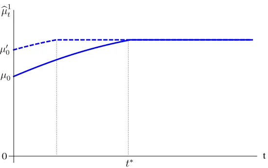
Figure 1: Market’s belief and threshold time in the equilibrium of the bad news setting. Parameters areµ₀= 0.6, x= 0.75, λB= 1.8, R= 1.2, andr= 1.

Proposition 1 (Bad news setting). The equilibrium is unique. There exists a threshold time t∗ _≥₀_{such that the agent starts working at time 0, stops immediately if he fails at} _{t < t}∗_{, and}

continues working otherwise.

The market’s time-t belief conditional on the agent not having stopped by tis_bµ_t1 =µ_t fort_≤t∗

andµ_b1_t =µ_t∗ for t > t∗. The market’s time-t belief conditional on the agent having stopped by

t is 0, both on and off the equilibrium path.

The threshold time satisfies t∗ = ∞ if R ≤ −(x−λB) and t∗ = 0 if R ≥ −(x−λB)/µ0. If

−(x−λB)< R <−(x−λB)/µ0, then t∗ is given by

x−λB+µt∗R = 0. (7)

The equilibrium is characterized by a threshold time t∗ _≥ _{0 such that the agent stops}

at t if and only if a failure occurs at t and t < t∗. As discussed above, if R ≤ −(x−λB),

the equilibrium implements the first best, so t∗ = ∞ in this case. At the other extreme, if R≥ −(x−λB)/µ0, the agent always prefers to continue after failure, so t∗ = 0. The threshold

time is interior when−(x−λB)< R <−(x−λB)/µ0. In this case, the threshold time is the

time t∗ _{at which the agent is indifferent between stopping and continuing given that he has}

failed at t∗_{, given by equation (}₇_). _{Figure 1} _{illustrates the market’s equilibrium belief} _b_µ1 t in

an example with such an interior time t∗_.

The agent’s time-0 expected payoff from following the equilibrium strategy with threshold

(15)

time t∗ _is

π0(t∗) = µ0

x r +

Z t∗

0

e−rtµ_tRdt+e−rt∗µt∗R r

+ (1₋µ₀)

Z t∗

0

e−(r+λB)t_(x₋_λ

B+µtR)dt+e−(r+λB)t

∗(x−λB+µt∗R)

r

.

A sufficient condition for the agent to prefer following the equilibrium strategy rather than never working is π0(0) ≥ µ0R/r, which is satisfied by Assumption 1. In fact, given this

assumption, we can show that a no-work equilibrium (in which the agent never works on the project) does not exist. Intuitively, if a no-work equilibrium exists, it exists when the market’s beliefs are such that the agent’s reputation benefit from starting the project at time 0 is minimized. These beliefs correspond to the market expecting the agent to never stop once he starts working — so thatµ_b1_t =µ₀ for all t > 0 — and believing that the agent has failed if he ever stops.21 _{However, since the agent’s payoff from never working is} _µ

0R/r, it is clear

that underAssumption 1 the agent would prefer working forever to never working.

We can therefore show that the unique equilibrium is the equilibrium characterized in

Proposition 1. Suppose the agent’s career concern R is intermediate so that the threshold time t∗ _{is interior. Applied to the banking industry, the equilibrium says that a bank will}

stop rolling over a borrower’s debt if it learns early enough that the borrower is in distress. However, as the borrower repays and the bank keeps lending, the bank’s reputation increases. At some point, the reputational cost of admitting losses becomes high enough that the bank would choose to roll over a bad loan.22

Since a bank that keeps the debt until time t∗ _{continues refinancing it regardless of its}

value, the market learns no information about the quality of the bank’s loans after this time. Yet, note that the market expects more losses as time goes by. Specifically, let ηt be the

probability that the agent has failed by time t given that the agent has not stopped by t. In the first best, η_t = 0 for all t _≥ 0, since the agent stops immediately when a failure occurs. Instead, in an equilibrium with finite threshold timet∗_, _η

t= 0 for t < t∗ and

η_t= (1₋µ_t∗)

1₋e−λB(t−t∗)

21_{Recall that the agent has no private information at time 0; hence, the market’s belief cannot change upon} observing the agent’s start decision.

(16)

fort _≥t∗_{, since the agent does not stop upon failing after} _t∗_.

Corollary 2. The market’s belief that the agent has failed conditional on the agent not having stopped is increasing over time.

For the banking industry, these equilibrium dynamics have the flavor of a “crisis buildup”: banks continue rolling over (bad) loans and the market becomes increasingly concerned that banks are accumulating losses.

2.3 Expected quality and information

Social welfare in an equilibrium with threshold timet∗ _{is equal to}

S0(t∗) =µ0

x

r + (1−µ0)(x−λB)

1−e−(r+λB)t∗

r+λB

+ e−

(r+λB)t∗

r

. (8)

Note that S0(t∗) coincides with S0F B in equation (4) if and only if t∗ = ∞. Clearly, ceteris

paribus, welfareS0(t∗) decreases, and the distortionS0F B−S0(t∗) increases, when the threshold

time t∗ _declines.

The welfare effects of career concerns are then immediate from Proposition 1. The higher is the agent’s concern for his reputationR, the lower is the equilibrium threshold timet∗_{, and}

hence the lower is social welfare and the larger is the distortion relative to first best.

What are the welfare effects of an increase in the expected quality of projects? Suppose the prior probability of a good project, µ0, increases. First-best welfare then naturally goes

up. Moreover, since the agent’s career concern distorts actions away from first best only when the project is bad, an increase inµ0 has a direct effect of decreasing the distortion for any fixed

threshold timet∗_{. However, an increase in}_µ

0 also reduces the equilibrium threshold time t∗:

when expected project quality is higher, the agent’s reputation loss from ending the project at any time tincreases, and the time t∗ _{after which the agent prefers to continue upon failing}

decreases. We show that in net, an increase inµ₀ increases welfare, but, for interior solutions, it also increases the distortion generated by the agent’s career concern.

Proposition 2 (Expected quality in bad news setting). Suppose parameters _{µ₀, x, λB, R, r}

satisfy ₋(x₋λB)/µ0 > R >−(x−λB) (so the equilibrium features t∗ ∈(0,∞)) and consider

changes in µ₀ that preserve this property and Assumption 1. An increase in µ₀ increases welfare but it also increases the distortion relative to first best.

(17)

continuation payo↵ from continuing is

Z 1

t

e r(⌧ t) x B+ ˆp1⌧R d⌧ . (15)

The agent is willing to stop at any timetat which he fails only if (14) exceeds (15) for all t >0, or, equivalently, since limt!1pˆ1t = 1, only if

(1 pˆ0)R+ (x B)0. (16)

In addition, the first best requires that the agent start working at time 0; our assumption that x (1 µ0) B 0 ensures that the agent indeed has incentives to do so (as elaborated infn. 4 below).

Condition (16) is satisfied if the agent’s career concern is sufficiently small. If, on the other hand, R is large enough that this condition fails, there will exist a timet > 0 at which the agent will not want to stop upon failure: the agent’s cost of losing his reputation exceeds his cost of continuing working on a bad project.

Proposition 2 (Bad news). The equilibrium is unique. If (1 pˆ0₎_R_{+ (}_x

B)0, the equilibrium implements the first best. If (1 pˆ0)R+ (x B)>0,

the equilibrium is a threshold equilibrium with threshold timet⇤ ₀_{: the agent} starts working at time 0, stops immediately upon failure if he fails at t < t⇤_, and continues working forever otherwise. If (p0 pˆ0)R+ (x B) 0, then

t⇤ _{= 0}_{; otherwise,} _t⇤ _{is given by}

ˆ

p1

t⇤ pˆ0 R+ (x B) = 0. (17)

In a threshold equilibrium with threshold timet⇤_{, the agent stops at a time}

t if and only if a failure occurs at t and t < t⇤_{. The market’s time-}_t _belief that the agent’s ability is high is ˆp0 _{if the agent has stopped by} _t_{, ˆ}_p1

t if the agent has not stopped by t and t  t⇤_{, and ˆ}_p1

t⇤ if the agent has not stopped by t and t > t⇤_{, where ˆ}_p0 _{and ˆ}_p1

t are given by (12) and (13) respectively. If (p0 pˆ0)R+ (x B) 0, the agent always prefers to continue after failure,

12

R bµ1t µt +x+µt G ✓

Vt

R r

◆

= 0. (1)

˙

b

µ1tR= ˙µtR µ˙t G ✓

Vt R

r

◆

µt GV˙t. (2)

We rewrite (2) by substituting with ˙Vt = bµ1tR+r(Vt v), v = 1 + G_r+x, ˙µt =

µt(1 µt) G, and (1):

˙

b

µ1tR= [2 Gµt+r G](bµ1tR+x) +µt(r+ G) ( G R). (3)

Consider first the case in whichR+x >0> µ0R+x, so thattis finite andtinfinite. The di↵erential equation has a closed-form solution:

b

µ1t =

ert_Kµ

t(1 µt)

µ0(1 µ0) 1

rR[µt( G R)[r+ G(1 µt)] +rx], (4)

where K is a constant given by the boundary conditions. Substituting (4) into Vt =

v+RR_t1e r(s t)

b

p1

Vt=v+

ert_KRµ t

Gµ0(1 µ0) 1

r[x+µt( G R)].

The value of tdepends on µ0. Using the expression for Vt above, K and t can be

b

µ1t = µ0, (5)

Vt

R r

◆

= 0. (6)

µ0 µ00 µ000

1 The agent’s indi↵erence condition is now

R bµ1_t µ_t +x+µ_{t G}

✓

Vt

R r

◆

= 0. (1)

˙

b

✓

Vt

R r

◆

µ_{t G}V˙t. (2)

We rewrite (2) by substituting with ˙Vt = µb1tR+r(Vt v), v = 1 + G_r+x, ˙µt =

µ_t(1 µ_t) G, and (1):

˙

b

Consider first the case in whichR+x >0> µ₀R+x, so thattis finite andtinfinite. The di↵erential equation has a closed-form solution:

b

µ1_t = e

rt_Kµ

t(1 µt)

µ₀(1 µ₀)

1

rR[µt( G R)[r+ G(1 µt)] +rx], (4)

whereK is a constant given by the boundary conditions. Substituting (4) into Vt =

Vt=v+ e

rt_KRµ

t

Gµ0(1 µ0) 1

r[x+µt( G R)].

The value of t depends on µ₀. Using the expression for Vt above, K and t can be

b

µ1_t = µ₀, (5)

R(µ₀ µ_t) +x+µ_{t G}

✓

Vt

R r

◆

= 0. (6)

µ0 µ00 µ000

1

R _bµ1t µt +x+µt G ✓

Vt

R r

◆

= 0. (1)

˙

b

✓

Vt

R r

◆

µ_{t G}V˙t. (2)

We rewrite (??) by substituting with ˙Vt = µb1tR+r(Vt v),v = 1 + G_r+x, ˙µt =

µ_t(1 µ_t) G, and (??):

˙

b

µ1_tR= [2 Gµt+r G](µb1tR+x) +µt(r+ G) ( G R). (3)

Consider first the case in whichR+x >0> µ0R+x, so thattis finite andtinfinite.

The di↵erential equation has a closed-form solution:

b

µ1t =

ert_Kµ

t(1 µt)

µ₀(1 µ₀)

1

rR[µt( G R)[r+ G(1 µt)] +rx], (4)

whereK is a constant given by the boundary conditions. Substituting (??) intoVt =

Vt=v+

ert_KRµ t

Gµ0(1 µ0)

1

r[x+µt( G R)].

The value of t depends on µ0. Using the expression for Vt above, K andt can be

b

µ1_t = µ0, (5)

Vt

R r

◆

= 0. (6)

b

µ1t

µ_t x R x Gv 1

In[35]:= Plot@8muhat1L@sD<, 8s, 0, 1.75<, PlotRangeØ8-0.05, 1.1<,

BaseStyleØ8FontSizeØ14<, AxesLabelØ8"t", ""<, PlotStyleØ88Blue, Thick<<, TicksØ88<, 8<<D

Plot@8muhat1L@sD, muhat1H@sD<, 8s, 0, 1.75<, PlotRangeØ8-0.05, 1.1<, BaseStyleØ8FontSizeØ14<, AxesLabelØ8"t", ""<,

PlotStyleØ88Blue, Thick<, 8Blue, Thick, Dashed<<, TicksØ88<, 8<<D

Out[35]=

t

Out[36]=

t

4 Examples Bad News.nb

1 Compute stopping policy

Discretize time in periods of

dt

length, so

t

_{2 {}

0 , dt,

2 dt, ...

_}

. Assume

t

F B

and

t

are on the grid, i.e.,

t

F B

/dt

and

t/dt

are integers. The probability that a good project succeeds over a period of length

dt

is

G

dt

. Then the probability that a good project succeeds before time

t

is: 1

(1

G

dt

)

t dt

.

We know that the agent continues for sure until time

t

. At that point,

_b

µ

1_t

=

µ

₀

. Now take

µ

_b

1_t₊_dt

.

We know what this is, and we want to compute the probability that the agent continues over [

t, t

+

dt

]

absent success. Call

_t

dt

the probability that the agent drops over [

t, t

+

dt

] absent success. Then

b

µ

1_t₊_dt

=

µ

₀

h

1 (1

G

dt

)

t dt

i

+

µ

₀

(1

G

dt

)

t

dt

(1

_t

dt

)

µ

₀

h

1 (1

G

dt

)

t dt

i

+ (

µ

₀

(1

G

dt

)

t

dt

+ 1

µ

₀

)(1

_t

dt

)

Call

_t₊_dt

dt

the probability that the agent drops over [

t

+

dt, t

+ 2

dt

] absent success. Then the

probability that an agent who has a bad project will stay until time

t

+ 2

dt

is

(1

_t

dt

)(1

_t₊_dt

dt

)

Now note that an agent who has a good project and had not succeeded by

t

and stayed till

t

+

dt

may have succeeded over [

t, t

+

dt

], in which case he stays from

t

+

dt

on. The probability that he

succeeded over that interval is

G

dt

. Then the probability that an agent who has a good project and

had not succeeded by time

t

will stay until

t

+ 2

dt

is

(1

_t

dt

)[

_G

dt

+ (1

_G

dt

)(1

_t₊_dt

dt

)]

We compute

b

µ

1_t₊₂_dt

=

µ

0

h

1 (1

G

dt

)

t dt

i

+

µ

₀

(1

G

dt

)

t

dt

(1

_t

dt

)[

_G

dt

+ (1

_G

dt

)(1

_t₊_dt

dt

)]

"

µ

₀

h

1 (1

G

dt

)

t dt

i

+

µ

₀

(1

G

dt

)

t

dt

(1

₁

dt

)[

_G

dt

+ (1

_G

dt

)(1

_t₊_dt

dt

)]

+(1

µ

₀

)(1

_t

dt

)(1

_t₊_dt

dt

)

#

And we can continue doing this for

t

+ 3

dt

, etc.

To check:

Confirm that as we take

dt

smaller and smaller, the change in

_t

dt

also gets smaller

and smaller, so these probabilities converge to the continuous time limit. To see this, let

t

be defined

as:

t dt

= 1, and for

t

,

t

= ⇧

t⌧=t

(1

⌧

dt

) = (1

t

dt

)(1

t+dt

dt

)(1

t+2dt

dt

)

...

(1

t+ndt

dt

)

[image:17.612.171.446.72.245.2]

for

t

+

ndt

=

t

. Plot

t

for di↵erent values of small

dt

(i.e., plot di↵erent lines on the same graph,

with

t

on the x-axis, starting at

t

=

t

dt

).

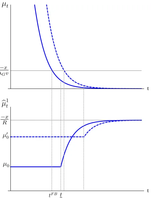
Figure 2: Effects of an increase in µ₀ in the equilibrium of the bad news setting. Parameters are the same as inFigure 1, withµ0₀= 0.8.

if failure first occurs after the market’s belief has reached µ_t∗, given by (7). Observe that

µ_t∗ is independent of µ₀. Hence, once the market’s belief reaches µ_t∗, the probability that

the project is bad (1−µ_t∗), and thus the expected losses the agent generates by continuing,

are also independent of µ0. An increase in µ0 however reduces the time that it takes for the

market’s belief to reach µt∗; that is, as illustrated in Figure 2, t∗ decreases with µ0. This

reduction int∗ has two implications: first, the agent is less likely to fail byt∗, and second, the losses occur earlier in time and are thus less heavily discounted. As a consequence, both the probability of a distortion and the present value of the distortion increase whenµ₀ goes up.

Proposition 2 considers parameters under which the equilibrium features a distortion but the distortion is not extreme (i.e. ₋(x₋λB)/µ0 > R > −(x−λB)). If instead the agent’s

reputational concernRis small enough that the equilibrium implements the first best (i.e.R <

−(x−λB)), then distortions are zero regardless ofµ0 and welfare increases withµ0. Similarly,

ifR is large enough that the equilibrium distortion is already extreme (i.e.−(x−λB)/µ0 < R),

then an increase in µ0 has no effect on the behavior of the agent (who never abandons the

project) and the distortion decreases withµ0. Since our interest is in studying the pattern of

distortions, and the effects in the latter case are simply due to a corner solution when R is too large relative toµ₀, we focus on the intermediate case.

The results inProposition 2contribute to the discussion mentioned in the Introduction on how banks’ behavior and distortions vary in good versus bad times. During good times, the average quality of borrowers is higher than during bad times. However, because the market’s expectation of loan quality is then higher, banks’ reputational loss from recognizing bad loans

(18)

is also larger.23 _{Proposition 2}_{shows that, as a result, career-concerned bank managers will be}

more likely to roll over their bad loans during good times compared to bad times. Furthermore, despite the proportion of bad borrowers being smaller, banks will in expectation accumulate more bad debt during good times. Consistent with the empirical findings of Schularick and Taylor(2012), one may say that banks plant the seed for the next crisis during boom periods. Would information about project quality ameliorate the welfare distortions due to career concerns? After all, it is because the quality of the project is uncertain that career concerns lead to distorted behavior. Suppose that it is possible to release a public signal at time 0 that refines the agent and market’s common prior on the project,µ0. Absent career concerns, the

signal either keeps welfare unchanged — if it does not affect the decision of whether to start the project at time 0 — or increases welfare — if it does affect this start decision. However, when the agent is career-concerned, the signal also affects distortions: as implied byProposition 2, a high realization of the signal (i.e. a realization that increasesµ₀) may increase the distortion relative to first best, whereas a low realization may lower this distortion. We find that the net welfare effect, and thus the value of information, can be negative.

Proposition 3(Information in bad news setting). Suppose parameters_{µ₀, x, λB, R, r}satisfy −(x₋λB)/µ0 > R >−(x−λB)(so the equilibrium features t∗ ∈(0,∞)) and consider a public

signal that refines µ₀ at time 0 while preserving this property and Assumption 1 for all of its realizations. The signal increases the distortion relative to first best and lowers welfare. If instead the signal is perfect, it eliminates distortions and increases welfare.

The first part of the proposition considers an imperfect public signal that keeps the first-best start decision, and thus first-first-best welfare, unchanged. As in Proposition 2, we focus on intermediate parameters (i.e. no corner solutions). To illustrate the effects of the signal on equilibrium welfare, suppose the signal is binary, i.e. it either increases the prior to µh

0 > µ0

or lowers it to µ`

0 < µ0. Let each realization be unconditionally equally likely, so that µ0 = 1

2 µ

h 0 +µ`0

. Building on our discussion ofProposition 2, the signal realization affects the time t∗ _{that it takes for the market’s belief to reach}_µ

t∗, after which the agent is no longer willing to

stop upon failure. The losses that the agent generates onceµ_t∗ is reached are independent of

µ₀; what matters is the probability of reaching µ_t∗ and how heavily the losses are discounted.

The probability of reachingµ_t∗ is equal to _µµ0

t∗ = 1 2

_µh 0 µt∗ +

µ` 0 µt∗

and is thus unchanged with the public signal. However, ift∗(µ₀) is the amount of time it takes to reach µ_t∗ from µ₀, then the

losses atµt∗ are discounted bye−rt ∗₍_µ

0), which is a convex function ofµ

0.24 This means that the

23_{Loan quality in reality also depends on the bank’s screening. This discussion assumes that screening does} not fully eliminate differences in loan quality between good and bad times.

24_{By equation (}₂_),_e−rt∗(µ₀)₌ µ₀

1−µ₀

1−µ_t∗

(19)

public signal increases the expected discounted losses (since 1 2(e−

rt∗₍_µh

0)+e−rt∗(µ`0))> e−rt∗(µ0)),

and as a consequence it reduces welfare.

Things of course are different if the public signal is perfect, as considered in the second part ofProposition 3. If the signal fully reveals the quality of the project at time 0, the agent’s actions provide no information to the market. Hence, in this case, a career-concerned agent has no incentives to distort his behavior, and the distortion relative to first best is eliminated. Since first-best welfare increases with a fully informative signal, it follows that equilibrium welfare also increases. Combined with the first part of the proposition, this result implies that the effects of information are non-monotonic: sufficient information is beneficial, but limited information is harmful.

Our results have implications for policy, especially when applied to the banking industry. Governmental authorities conduct supervisory exams on banks to produce information on expected loan performance, and have the choice of making this information publicly available or not. Since 2009, the US and Europe incorporated into their supervisory programs the use of stress tests, which are forward-looking exams with the goal of projecting left-tail risk (e.g.,

Hirtle and Lehnert, 2014). Unlike with more traditional exams, the US requires that the results of individual banks’ stress tests be publicly disclosed. In Europe, stress test results were not published in 2009 but public disclosure was required in subsequent years.

There is a current debate among practitioners and scholars on whether the results of banks’ stress tests should be publicly disclosed. Bernanke (2013) argues that disclosure provides valuable information to market participants and the public and promotes market discipline.

Goldstein and Sapra(2013) also find disclosure beneficial, although they discuss various risks and challenges associated with disclosure. Our goal is not to assess the different benefits and costs of disclosing banks’ stress test results, but rather to point out a potential pitfall in the view that information is always beneficial — a view that seems to be behind much of the support for stress tests and their public disclosure. Proposition 3 shows that information on loan quality can be detrimental: when imperfect, this information can exacerbate distortions due to bank managers’ career concerns and reduce overall welfare.

3 Good news

We contrast the bad news setting of Section 2 with a good news setting in which the agent learns about project quality from the arrival of a success: λG > λB = 0> x(withλG+x >0).