Probabilistic Modelling of Uncertainty with Bayesian nonparametric Machine Learning

(1)

A Thesis Submitted for the Degree of PhD at the University of Warwick

Permanent WRAP URL:

http://wrap.warwick.ac.uk/

128793

Copyright and reuse:

This thesis is made available online and is protected by original copyright.

Please scroll down to view the document itself.

Please refer to the repository record for this item for information to help you to cite it.

Our policy information is available from the repository home page.

For more information, please contact the WRAP Team at:

wrap@warwick.ac.uk

(2)

Probabilistic modelling of uncertainty with

Bayesian nonparametric machine learning

by

Charles Gadd

Thesis

Submitted to the University of Warwick

for the degree of

Doctor of Philosophy

School of Engineering

(3)

Acknowledgments

Foremost I would like to thank my supervisors, Dr Sara Wade and Dr Akeel Shah,

for their guidance, support, and stimulating discussions. I am also grateful to all my

colleagues, both within and outside the department, who have been involved with

this work.

I gratefully acknowledge the financial support from the EPSRC funding body

that has made completion of this doctorate possible. Additionally, data

collec-tion and sharing for the Alzheimer’s disease study was funded by the Alzheimer’s

Disease Neuroimaging Initiative (ADNI) (National Institutes of Health Grant U01

AG024904). I acknowledge the funding contributions of ADNI supporters (adni-info.

(4)

Abstract

This thesis addresses the use of probabilistic predictive modelling and

ma-chine learning for quantifying uncertainties. Predictive modelling makes inferences

of a process from observations obtained using computational modelling, simulation,

or experimentation. This is often achieved using statistical machine learning

mod-els which predict the outcome as a function of variable predictors and given process

observations. Towards this end Bayesian nonparametric regression is used, which is

a highly flexible and probabilistic type of statistical model and provides a natural

framework in which uncertainties can be included.

The contributions of this thesis are threefold. Firstly, a novel approach to

quantify parametric uncertainty in the Gaussian process latent variable model is

presented, which is shown to improve predictive performance when compared with

the commonly used variational expectation maximisation approach. Secondly, an

emulator using manifold learning (local tangent space alignment) is developed for the

purpose of dealing with problems where outputs lie in a high dimensional manifold.

Using this, a framework is proposed to solve the forward problem for uncertainty

quantification and applied to two fluid dynamics simulations. Finally, an enriched

clustering model for generalised mixtures of Gaussian process experts is presented,

which improves clustering, scaling with the number of covariates, and prediction

when compared with what is known as the alternative model. This is then applied

to a study of Alzheimer’s disease, with the aim of improving prediction of disease

(5)

Abbreviations

• AD . . . Alzheimer’s Disease

• ADNI . . . Alzheimer’s Disease Neuroimaging Initiative

• ANN . . . Artificial neural network

• ARD . . . Automatic relevance determination

• BNP . . . Bayesian nonparametric

• CN . . . .Cognitively normal

• DP . . . Dirichlet process

• EDP . . . Enriched Dirichlet process

• EMCI . . . Early mild cognitive impairment

• ESS . . . Elliptical slice sampling

• FD . . . .Finite difference

• GLM . . . Generalised linear model

• GP . . . Gaussian process

• GPLVM . . . Gaussian process latent variable model

• HMC . . . Hamiltonian Monte Carlo

• KDE . . . Kernel density estimation

• KL . . . Kullback-Leibler

• KLE . . . Karhunen-Lo`eve expansion

• LMCI . . . Late mild cognitive impairment

(6)

• MAP . . . Maximum a posteriori

• MC . . . Monte Carlo

• MCMC . . . Markov Chain Monte Carlo

• ML . . . Maximum likelihood

• MML . . . Maximum marginal likelihood

• MMSE . . . Mini-mental state exam

• PDE . . . Partial differential equation

• PM . . . Pseudo-marginal

• PMMC . . . Pseudo-marginal Monte Carlo

• PPCA . . . Probabilistic principal component analysis

• sGPLVM . . . Supervised Gaussian process latent variable model

• UQ . . . Uncertainty quantification

• VEM . . . Variational expectation maximisation

(7)

Notation

Within this section the nomenclature and notation commonly found throughout this thesis

is presented. Where interchangeable the letter ‘a’ is used. Notation not outlined here is

defined upon use.

Roman symbols

a: Vector

A: Matrix

a: Scalar

A: Vector space in which vector alies

ka: For some vectora∈ A, thenka is the dimension of the vector space

TaA: The tangent space (a linear subspace) of vector spaceAata

X: Dataset inputs

Y: Dataset outputs

D: Dataset{X, Y}

N: Number of samples in the training dataset

Greek symbols

θ,σ,β: The Gaussian process hyperparameters

Θ: The joint set of Gaussian process hyperparameters

(8)

Superscripts

a(i)_: _ith_{value in a series (e.g. Markov Chain, importance samples, etc.)}

aM L_: _{The maximum marginal likelihood estimate of hyperparameter} _a

Subscripts

ai: The ithelement of a vector

Ai: The ithrow of a matrix (e.g. Xi is the ithsample’s covariates)

A:,j: The jthcolumn of a matrix (e.g. X:,j is the jthcovariate of all samples)

Ai,j: The element of a matrix on the ithrow and jthcolumn

Other symbols

N: The Gaussian distribution

Dir: The Dirichlet distribution

Bern: The Bernoulli distribution

Ga: The Gamma distribution

Beta: The Beta distribution

GP: The Gaussian process

DP: The Dirichlet process

EDP: The enriched Dirichlet process

R_: _{The real numbers}

O: Big-O notation

Functions

K(_·,_·): A kernel function

Ka: A kernel function evaluated at points in A.

Ka∗: A kernel function evaluated between training and test points in A.

(9)

List of Tables

3.1 Simulated sinuoidal: Hyper-priors . . . 41 3.2 Simulated sinuoidal: Mean absolute errors . . . 44

5.1 Damped cosine: The number of VI estimated x-clusters within the two estimated y-clusters . . . 100 5.2 Damped cosine: Clustering summary statistics, predictive accuracy,

(13)

List of Figures

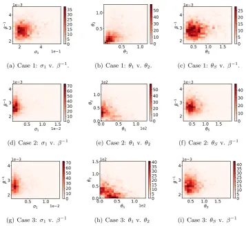
3.1 Simulated sinusoidal: Posterior distributions . . . 42

3.2 Simulated sinusoidal: Case 3 predictive distributions . . . 43

4.1 Emulator framework . . . 48

4.2 Simulated Darcy: Input model 1 log normalised error . . . 67

4.3 Simulated Darcy: Input model 1 predictive moments of the test point with highest error . . . 68

4.4 Simulated Darcy: Input model 1 predictive moments of the test point with median error . . . 69

4.5 Simulated Darcy: Input model 1 pdf of pressure head at a spatial co-ordinate . . . 70

4.6 Simulated Darcy: Input model 1 predictive moments of the pressure head moments . . . 71

4.9 Simulated Darcy: Input model 2 predictive moments of the test point with median error . . . 74

4.10 Simulated Darcy: Input model 2 pdf of pressure head at spatial co-ordinate . . . 75

(14)

4.15 Simulated Darcy: Input model 3 pdf of pressure head at spatial

co-ordinate . . . 80

4.17 Simulated Richards: Log normalised error and pdf of pressure head at spatial co-ordinate . . . 82

4.18 Simulated Richards: predictive moments of pressure head moments . 83 5.1 Damped cosine: y-cluster posterior similarity matrix . . . 99

5.2 Damped cosine: VI estimated y-clustering . . . 100

5.3 Damped cosine: x-cluster posterior similarity matrix within the two estimated y-clusters . . . 101

5.4 Damped cosine: y-cluster allocation probabilites . . . 102

5.5 Damped cosine: Predictive density . . . 104

5.6 Damped cosine: Empirical coverage . . . 105

5.7 ADNI: y-cluster posterior similarity matrix . . . 107

5.8 ADNI: VI estimated y-clustering . . . 107

5.9 ADNI: y-cluster posterior similarity matrix . . . 109

5.10 ADNI: VI estimated x-clustering within each y-cluster . . . 109

5.11 ADNI: Allocation probabilities as a function of MMSE and different diagnoses . . . 110

5.12 ADNI: Marginalised predictive density . . . 111

5.13 ADNI: Predictive density . . . 112

A.1 Simulated sinusoidal: Trace plots . . . 117

A.2 Simulated sinusoidal: Auto-correlation . . . 118

A.3 Simulated sinusoidal: Bivariate marginal latent posterior . . . 120

A.4 Simulated sinusoidal: Bivariate marginal latent posterior . . . 121

A.5 Simulated sinusoidal: Marginal latent posterior . . . 122

A.6 Simulated sinusoidal: Marginal latent posterior given ML . . . 123

A.11 Simulated sinusoidal: Case 1 predictive distributions . . . 128

A.12 Simulated sinusoidal: Case 2 predictive distributions . . . 129

(15)

List of Algorithms

1 Metropolis-Hastings algorithm with symmetric proposal distribution 18

2 Hamiltonian Monte Carlo algorithm (leap frog method) . . . 19

3 Elliptical slice sampling algorithm . . . 20

4 Gibbs sampling algorithm . . . 21

5 Pseudo-marginal Metropolis Hastings algorithm with symmetric pro-posal distribution . . . 23

6 Pseudo-marginal adaptive MH in Gibbs. . . 37

7 Elliptical slice sampler for the latent variables. . . 38

(16)

Chapter 1

Introduction

1.1 Motivation

Machine learning is the act of using algorithms and models which allow computers to ‘learn’ based on a set of experiences, where experiences often exist in the form of data. In this context, learning is the process of gaining an understanding of a task through the building of a computational model of training data. This learnt model can then be used to make predictions or decisions without requiring rules to make them being specifically programmed, as would be the case in a rule-based system. The work presented in this thesis lies in the domain of statistical machine learning, in which machine learning methods are combined with statistical techniques under the assumption of statistical regularity in the data. Specifically, the work presented here lies at the intersection of Bayesian nonparametrics (BNP) and machine learn-ing. The upshot of BNP machine learning is a natural probabilistic framework for an interpretable inclusion of uncertainties though probability theory, with the framework simplicity of Bayesian models, while being able to model the complexity of real world phenomena using nonparametrics. This approach can be used to infer unknown quantities, adapt models, learn from the data and make predictions.

(17)

that change each time the experiment is run. For example, an infinite number of dice rolls does not remove the stochastic nature of rolling a dice. Another common example is an arrow’s impact point which, given initial firing parameters, will vary due to seemingly random vibrations in the arrow shaft. In this case the uncertainty occurs due to the lack of knowledge. However, once this information can be obtained it becomes an epistemic uncertainty. Prevalent examples of uncertainty encountered when modelling include:

• Data noise. For example, from measurement imprecision, human error, or missing explanatory variables in the data set.

• Out of distribution/interpolation uncertainty. For example, in data-driven models predictions away from the training samples should have a higher pre-dictive uncertainty to reflect the reduced available information.

• Model structure/distributional uncertainty. For example, a model may as-sume heterogeneous noise, distributional form, regularity, stationarity, and a function’s smoothness or form. Additionally there may be approximations to a model which introduces further uncertainties.

• Model parameter uncertainty. For example, there may be a large number of parameters (and therefore models) which can explain the observed data. Similarly, in the nonparametric setting with an infinite dimensional parameter space, there is uncertainty associated with the choice of hyperparameters.

A principled approach to understanding, quantifying, reducing and modelling these uncertainties is critical for many scenarios. Obvious examples include any high risk decision making task where it is crucial that a model output can be trusted, such as in performing a medical diagnosis or assisted driving. These themes are core to this thesis and a deeper understanding allows us to answer many questions, such as whether a model can be trusted, if predictions are uncertain, or if approximations to a model are accurate.

(18)

1.2 Thesis structure

The first part of this thesis (chapter 2) introduces the fundamentals upon which this work builds. This includes a brief introduction to BNP modelling, two popular prior processes commonly used in BNP models and a brief introduction to some schemes used to perform posterior inference in these models.

Chapter 3 introduces a novel Bayesian framework for inference with a su-pervised version of the Gaussian process latent variable model (GPLVM). This is motivated by weaknesses in the use of: point estimates to hyperparameters; ap-proximations of the estimates, often through non-convex optimisation; and model approximations, through variational expectation maximisation. GPLVM is a hierar-chical model in which hyperparameters and latent variables are heavily correlated. The proposed framework overcomes these correlations using a collapsed Metropolis-within-Gibbs sampler, with an unbiased pseudo estimate for the marginal likelihood that approximately integrates over the latent variables and samples the hyper-parameter posterior. Conditional on these samples, the framework continues by uncollapsing the model with elliptical slice sampling (ESS) to explore the posterior of the latent variables. The procedure is demonstrated on simulated examples, show-ing the ability to capture uncertainty and multimodality of the hyperparameters. Additionally, the approach improves the accuracy of predictions when compared with the state-of-the-art inference techniques for GPLVM, which often come with the aforementioned weaknesses.

Following this, chapter 4 develops a surrogate modelling approach to regres-sion in high dimenregres-sional output spaces which lie on a manifold. This is then used to construct a framework to solve the forward problem of uncertainty quantification (UQ), in which input uncertainty is propagated through a model to predict the un-certainty in the system response. The approach obtains a lower dimensional latent representation of sample outputs using a feature extraction step using local tangent space alignment (LTSA), a nonparametric (but non-Bayesian) approach to mani-fold learning. These extracted features can then be used in conjunction with BNP Gaussian process (GP) emulation. This is then demonstrated on groundwater flow models involving a stochastic input field (e.g. the hydraulic conductivity) to capture the output field (e.g. the pressure head). A Karhunen-Lo`eve expansion (KLE) for a log-normally distributed input field is used. Two examples are presented to demon-strate the accuracy: a Darcy flow model with contaminant transport in 2 spatial dimensions and a Richards equation model in 3 spatial dimensions.

(19)

partitions the input space into regions where stationary and heterogeneous noise assumptions of the GP must only hold in each region. What is known as an alter-native model is presented, where the joint distribution of the inputs and targets is modelled explicitly. Whilst this modelling choice gives the ability to handle missing data and answer inverse problems, the local input model causes 1) the model to scale poorly with increasing input dimension and 2) the creation of an unnecessary number of experts, degrading the predictive performance and increasing uncertainty. To address the former, local independence assumptions of the inputs are made. This also allows for the inclusion of multiple input types. For the latter, the enriched Dirichlet process is utilised, allowing for a nested partitioning scheme and an analyt-ically computable allocation rule. This allows the development of efficient sampling algorithms for posterior inference. These advantages are demonstrated on a highly non-linear toy example with increasing input dimension and an Alzheimer’s chal-lenge to predict decline in cognitive impairment.

1.3 Associated publications and software

• The work presented in chapter 3 is based on Gadd et al. [2018] (in preparation). This paper presents a scheme for full Bayesian inference for the supervised GPLVM, which can be generalised to other models, such as the deep Gaussian process.

• The work presented in chapter 4 is based on Gadd et al. [2018]. This paper uses GP emulation for UQ tasks in a highly non-linear ground water flow problem, where the output space is high dimensional.

• The work presented in chapter 5 is based on work in preparation, where an enriched mixture model of generalised GP experts is presented.

(20)

Chapter 2

Pre-requisites

This chapter serves as a gentle introduction to the topics this thesis builds upon. The following sections introduce Bayesian nonparametric models; review two of the most popular priors (the Gaussian and Dirichlet process) and introduce some methods used to perform Bayesian inference in this family of models.

2.1 Bayesian analysis

Bayesian analysis is a self-contained paradigm for statistics that approaches un-known parameters probabilistically, treating them as random variables and exam-ines properties of the unknown random parameters conditioned on a set of observed data samples. Conversely, classical (frequentist) approaches treat parameters as unknown but fixed values and aim to find estimators of the fixed parameters with desirable properties that average over all potential data samples.

(21)

the confidence level, which is subjectively chosen by the practitioner. This relies on an asymptotic approximation, but the Bayesian approach provides inferences that are conditional on the data and are exact.

In almost all statistical problems, not using prior information can lead to obtaining weak or nonsensical results. The Bayesian paradigm allows for a natural, well-defined and more interpretable inclusion of prior information, which requires an appropriate prior distribution to be chosen. However, this choice is not always obvious. Two different practitioners may sometimes disagree and there may be unforeseen consequences in a prior choice (see the 8-schools example in Gelman et al. [1995] or section 3 of Gelman [1996]). However, a completely subjective prior specification is challenging, and in practice, priors are often chosen to balance com-putational considerations with prior elicitation.

2.2 Nonparametric modelling

A statistical model consists of a set of probability measures on the sample space. In a parametric setting, the statistical model is assumed to be indexed orparametrised, by some finite set of parameters. However, in this setting we must ascertain whether the data generating distribution belongs to a parametric model. Often, we do not have such knowledge. Model selection approaches compare various parametric mod-els through a trade-off between model complexity and goodness of fit.

Nonparametric models provide an alternative approach by removing the finite dimensional assumption of parametric models. Specifically, the number of param-eters (model complexity) does not need to be specified a priori and is allowed to grow with the sample size. This is automatically inferred from a finite data set, with an additional benefit that although one maya priori believe that a population requires infinite parameters, a finite subset may only require a finite number.

(22)

2.3 Gaussian process

Definition 1. A Gaussian process is a collection of random variables, such that any finite subset has a multivariate normal distribution with consistent parameters.

Gaussian processes (GPs) are stochastic processes used for inferring non-linear and latent functions. They are defined as a family of normally-distributed random variables, indexed in this case by the input variable(s). In Bayesian in-ference, GPs are functionals, used as a prior probability distribution over function space, defined fully by a process mean and a symmetric positive definite covariance function. The latter of which is defined by a kernel function, which produces a Gram matrix when evaluated at the observed inputs. Kernel methods such as these are well-established tools for analysing the relationships between input data and corresponding outputs of complex functions. Kernels encapsulate the properties of a function in a computationally efficient manner. Additionally, they provide flexi-bility in terms of model complexity (the functions used to approximate the target function) through variation of the functional form and parameters of the kernel. An introduction of GPs is given in Rasmussen [2004].

These priors over function space excel when data is scarce or corrupted since they make strong a priori assumptions with regards to the relationship between datum and on the functions they learn. In making these assumptions, inference or optimisation can be performed over a reduced model space. This is in keeping with the ‘no free lunch’ theorem of computational complexity and optimisation, which states that the cost of inference/optimisation is the same for any method when averaged over all problems in that class. However, by using informed prior knowledge, one can choose a model which better matches the problem, (Wolpert and Macready [1997]).

Gaussian processes have found uses in numerous machine learning tasks, including supervised learning (where the objective is to learn relationships between inputs and outputs, e.g. regression and classification), unsupervised learning (where the objective is to learn the structure of a data set, e.g. manifold learning and dimensionality reduction), and reinforcement learning (where a goal is achieved by associating a positive action on an agent with a reward).

(23)

as the function space perspective as the distribution is specified directly on the unknown function. Alternatively, they can be introduced using weight spaces as a Bayesian generalisation to ridge regression and then extending further by projecting inputs into a higher dimensional space using a set of basis functions where linear relations can then be found. In this setting, the kernel is expressed as the inner product between the basis functions (known as thekernel trick), which is the basis of kernel methods. The GP is then obtained after marginalising over the weights. This is known as the weight space perspective, as the distribution is specified on the weights in the basis function expansion, which marginally leads to GP distribution on the function. For mathematical details of this perspective the reader is referred to Rasmussen [2004].

Prior over function space

In this section the function space perspective is presented, where a prior is specified directly on the unknown function. Consider a set of N observed covariates X _∈

RN×D _{lying in a}_D_{-dimensional vector space}_X_{, with corresponding vector}_f _∈RN_of

scalar function values. A mean function1 _{is denoted} _µ _: _RD _→ _R _{and symmetric} positive definite covariance (kernel) function is denoted K(_·,_·) : RD _×RD _→ R_,

with the consequent Gram matrix K(X,X)∈RN×N_{, of a real process}_f₍_X_{) as:}

µ(X) =E_[_f₍X)],

K X,X′=Eh₍_f₍_X₎₋_µ₍_X_{)) (}_f₍_X₎₋_µ₍_X₎₎Ti_,

(2.1)

and write the GP prior over function space as:

f_|X_{∼ N}(µ(X), K(X,X)),

f(_·)_{∼ GP}(µ(_·), K(_·,_·)). (2.2)

where _X is the indexing set of possible inputs to the Gaussian process. Here and throughout, N(_·,_·) denotes a normal distribution, in which the first argument is the mean vector and the second is the covariance matrix. Additionally GP(·,·) denotes a GP, in which the first argument is the mean function and the second is the covariance (kernel) function. A random Gaussian vector of function values can be generated by sampling the multivariate Gaussian distribution at a finite number of points in _X.

Consequently, two function valuesf(Xi) and f(Xj) evaluated at points in

(24)

the indexing set are jointly Gaussian with meanµ= [µ(Xi), µ(Xj)] and covariance [Kii, Kij;Kji, Kjj], where the shorthand notation K(Xi,Xj) = Kij is used. The following two properties then apply. Given a random vector A _{∼ N}(µ,Σ) in n -dimensional space then:

Property 1. The marginal distribution is Gaussian. If we decompose A by

split-ting the finite indexing set into two disjoint subsets {{i},{j}}, such that A =

[ai,aj], µ = [µi,µj] and Σ = [Σii,Σij;Σji,Σjj], then ai ∼ N(µi,Σii), and

aj ∼ N(µj,Σjj).

Property 2. The conditional distribution is Gaussian. Given the decomposition

above, ai|aj ∼ N

µi+ΣijΣ−jj1(aj−µj),Σii−ΣTijΣ−jj1Σij

.

The existence of the GP is obtained from the Kolmogorov Extension Theorem (as an extension from the a consistent collection of finite dimensional distributions to a stochastic process) and the marginalisation property of the Gaussian distribution. Having defined this Gaussian process prior over function space, it is then possible to make inferences on the distribution over functions conditioned on a training set. The GP implies a joint Gaussian prior distribution over the function between training points and an unseen point:

"

f

f(x) #

∼ N hµ(X)T , µ(x)iT ,

"

K(X,X), K(X,x)T

K(X,x), K(x,x) !#

(2.3)

Following from the conditional property 2, we can easily obtain the analytic conditional distribution of the test function valuef, atx given observationsf:

f(x)|f _{∼ N}(m1(x), c1(x))

m1(x) =µ(x) +K(x,X)K(X,X)−1(f−µ(X))

c1(x) =K(x,x)−K(x,X)K(X,X)−1K(x,X)T

(2.4)

with Gaussian process posterior over function values:

(25)

The likelihood

In most modelling scenarios the true underlying function values are not known, but instead their noise corrupted values y =f(X) +η. In this case the standard ap-proach is to assume that the noise is additive, independent and identically Gaussian distributed,η_{∼ N} 0, β−1_I

N, leading to a factorised Gaussian likelihood:

p(y|f) =N y|f, β−1IN= N

Y

n=1

N yn|fn, β−1, (2.6)

Gaussian marginal likelihood, and Gaussian process marginal model:

p(y|X) = Z

p(y|f)p(f|X)df

y(_·)_{∼ GP} µ(_·), K(_·,_·) +β−1δ₍_·_,_·₎,

(2.7)

wherep(y_|X) is the marginal likelihood,p(y_|f) is the likelihood,p(f_|X) is the prior and β−1δ₍_·_,_·₎ is as a white noise kernel (also known as a nugget in this context). This kernel is a Kronecker-delta function scaled by a positive constant. An element of this kernel is then equal to the constant if both arguments are equal and zero otherwise. With this Gaussian likelihood, an analytic posterior GP over functions (and subsequent predictive distribution) is obtained:

f(·)|y∼ GP(m2(·), c2(·))

f(x)_|y_{∼ N}(m2(x), c2(x))

m2(·) =µ(·) +K(·,X) h

K(X,X)−1+β−1IN

i

(y₋µ(X))

c2(·) =K(·,·)−K(·,X) h

K(X,X)−1+β−1IN

i

K(·,X)T

(2.8)

and predictive posterior process over outputs, given newx:

y(_·)_|y_∼GP m2(·), c2(·) +β−1

y(x)|y_∼N m2(x), c2(x) +β−1

(2.9)

(26)

Alternative likelihoods may also be used. For example in binary (0,1) clas-sification, where the objective is to predict the probability that y = 1, one could transform the latent function through sigmoid (logistic), cumulative normal (probit) or (robust) threshold likelihood. Another example is count data for non-negative and discrete values, where latent functions are transformed to ensure positive sup-port and then used as a rate parameter in a Poisson distribution.

When a GP prior is coupled with a non-Gaussian likelihood, an analytically tractable marginal likelihood or posterior process over outputs is no longer avail-able. Stochastic approximations (such as Markov chain Monte Carlo (MCMC)), or deterministic approximations of integrals (such as Expectation Propagation, Laplace approximation or Variational approximation) must then be used to obtain an ap-proximation to the non-Gaussian joint posterior process of latent functions.

The Laplace approximation is fast, but gives a poor approximation if the mode does not well describe the posterior (for example when using the Bernoulli pro-bit likelihood). Expectation Propagation works very well under certain likelihoods and allows for sparse approximations but is otherwise slow, requires the ability to match moments and there can be convergence problems for some likelihoods. Vari-ational methods can also give sparse approximations and give a principled approxi-mation by optimizing a measure of divergence between the approxiapproxi-mation and true distribution. However, these approximations often require factorisation assumptions to avoid a high dimensional integral. A comparison between different deterministic approximations and MCMC methods for GP classification can be found in Nickisch and Rasmussen [2008]. From this point only GPs with Gaussian likelihoods are discussed, where posterior inference is analytically tractable.

2.3.1 Kernels

The mean and covariance (kernel) of the stochastic process encapsulate prior as-sumptions on the latent function form. The kernel is a function that maps pairs of inputs to the positive real line, usually based on distance and conditional on a set

ofhyperparameters θ.

(27)

space):

K x,x′=hφ(x), φ x′i. (2.10) Consequently the feature map must exist for a kernel to be valid. Mercer’s theorem gives a principled approach to ensure the existence of these feature maps for a kernel - satisfying Mercer’s condition ensures a kernel’s Gram matrix is positive-semi definite, which is enough to ensure existence (Cortes and Vapnik [1995]). This process of replacing inner products in the input space with a kernel representing the inner product in the feature space (the kernel trick) allows for flexible and computationally efficient measures of correlation.

The covariance between evaluations of the unknown function at any pair of inputs in a GP is measured using kernels. Valid kernels lead to symmetric, semi-positive definite covariances. The kernel choice (including hyperparameters) constrain the family of functions which can be modelled. Consequently the kernel encodes our prior belief of the function to be modelled. When using a GP, the choice of kernel has a significant impact. For example, the squared exponential kernel (otherwise known as theexponential quadraticorradial basis function) makes strong assumptions of the function’s smoothness. Using this kernel, the covariance between theith andjth sample is given by:

K(xi,xj|σ, l) =σ2exp

( −₂1_l

D

X

d=1

(xi,d−xj,d)2

)

, (2.11)

whereσ denotes the signal variance controlling the average distance of the function away from its mean, andldenotes the lengthscale controlling how fast the function changes with respect to changes in the input2. This kernel is infinitely differentiable, and consequently only suitable for learning very smooth functions. A number of alternative kernels and a detailed discussion of their construction and application is given in Duvenaud [2014]. The periodic kernel is useful when the function repeats itself, but may not result in a flexible model, and a Mat´ern kernel is useful when we expect less smooth functions given it is _⌊ν_⌋-times differentiable, where ν is a smoothness parameter.

We can increase the flexibility of these kernels by allowing each input di-mension its own lengthscale. In doing this an automatic relevance determination

(ARD) effect occurs (MacKay [1994], Rasmussen [2004]), where less relevant dimen-sions have larger lengthscales, and consequently the covariance depends more on the distance between more significant covariates. Further flexibility can be obtained by

(28)

using a combination of kernels. Common operators on kernels include:

1. Addition. This can be seen as anOR operator, where two input vectors are correlated if they are similar by either kernel. 3

2. Multiplication. This can be seen as a AND operator, where two vectors are correlated if they are similar by both kernels.

Similarity is quantified by a measure of distance between covariates. In both cases, each kernel may be a function of all or a subset of covariates, where each kernel has a different form. Commonly a white noise kernel is added in this way. This models the assumption that data is corrupted by random fluctuations (such as measurement error), and inclusion of this noise term prevents over-fitting and ensures our covariances are positive definite (invertible). However, it is often equivalent to include a nugget4, which is a scaled identity matrix, to the kernel through a likelihood.

2.4 Dirichlet process

Dirichlet processes (DPs) are a family of stochastic processes whose realisations are discrete probability measures. The parameters of the DP consist of a base dis-tribution H (the expected value of the process) and a concentration parameter α

(otherwise known as the scaling or mass parameter). Whilst the base distribution may be continuous, distributions drawn from the DP are almost surely (with prob-ability one) discrete and the concentration parameter determines the strength of belief in the base distribution, with the process degenerating to the base measure as the concentration parameter approaches infinity. The formal definition of the DP is:

Definition 2. Given a measurable spaceS, a base probability distribution H0 on S

and a positive real numberα, the Dirichlet process DP(α, H0) is a stochastic process

whose realization (i.e. a sample drawn from the process) is a probability distribution

over S, and such that for any measurable finite partition of S, denoted {Bi}ni=1, if

H∼DP(α, H0), then (H(B1), . . . , H(Bn))∼Dir(αH0(B1), . . . , αH0(Bn)).

Dirichlet processes were introduced by Ferguson [1973a] who used the Kol-mogorov Consistency Theorem to show their existence and described the Dirichlet

3_{For a GP this decomposition is maintained through Bayes rule, obtaining a posterior which can}

also be expressed as a sum of kernels.

4_{This naming convention has roots in geo-statistics where Gaussian process regression (then}

(29)

process posterior using Bayes rules and the conjugacy between the Dirichlet and multinomial distributions. Specifically, assuming

H _∼DP (α, H0) and θi|Hiid∼H fori= 1, . . . , n, (2.12)

conditioned thenobservations this posterior is:

H|θ1:n∼DP

α+n,αH0+

Pn i=1δθi

α+n

(2.13)

For explanation of this posterior process the reader is referred to Ferguson [1973a]. However, as realisations of the DP are discrete almost surely, it is common to convolute a known or specified density (that is absolutely continuous with respect to some measure Λ) with the DP to produce realisations that are absolutely contin-uous (with respect to Λ) almost surely Lo [1984]. This induces an infinite mixture model for flexible density estimation by making use of the DP as a prior for the unknown mixing measure. This approach is used in chapter 5. In this setting, the posterior distribution is no longer analytically tractable, however the hierarchical structure of the model can be used for stochastic or deterministic approximations.

Other mathematically equivalent representations of the DP have emerged which vary by their perspectives. Blackwell and MacQueen [1973] used de Finetti’s theorem to prove existence and introduced the Blackwell-MacQueen P´olya urn scheme which characterizes the marginal law of the exchangeable sequence (θ1, θ2, . . .), see also Pitman [1996]. In Sethuraman [1994b], a way of constructing a DP was in-troduced using a stick-breaking construction and finally Aldous [1985] inin-troduced the Chinese restaurant process construction. Each of these are briefly outlined in the following sections.

2.4.1 Blackwell-MacQueen

This representation draws motivation from the P´olya urn model, in which we have an urn containing balls of various colours. The model then proceeds by randomly selecting a ball, replacing it and adding an additional ball of the same colour. This sampling, in a ‘rich get richer’ fashion, underpins the Blackwell-MacQueen construc-tion.

(30)

H0 representing the prior belief of the distribution over colours. The first ball of colourθ1 is sampled from H0 and added to the urn, and the sampling process for

θn then proceeds as:

1. With probability proportional toα, drawθn∼H0 and add a ball of this colour in the urn.

2. With probability proportional ton₋1, draw a random ballifori= 1, . . . , n₋1 from the urn, observe its colour θi, and place it back to the urn and add an additional ball of the same colourθn=θi in the urn.

This produces a sequence of samplesθ1, θ2, . . . with predictive distributions:

θn|θ1:n−1∼

αH0+Pn_i₌₁−1δθi

α+n₋1 . (2.14)

Conversely, Blackwell and MacQueen [1973] start with the sequence of pre-dictive distribution in (2.14) and show that the sequence (θ1, θ2, . . .) is exchangeable, i.e for anyn_∈N_{, the joint distribution of the finite sequence is invariant to any finite}

permutation of the indices. Consequently by using the de Finettis theorem there must exist a distribution over a random probability measure such that, conditioned on this random probability measure, the sequence is independent and identically distributed, and this distribution is the Dirichlet process. As a result, it is proven that the Blackwell-MacQueen urn scheme is a representation of the DP and a way to construct it is obtained.

2.4.2 Chinese restaurant process

The Chinese restaurant process can be directly linked to the Blackwell-MacQueen urn scheme. We assume that there is a Chinese restaurant with an infinite number of tables. As the customers enter the restaurant they sit randomly to any of the occupied tables or they choose to sit at an empty table.

The process defines a distribution on the space of partitions of the positive integers. We start by drawingθ1, . . . , θnfrom the Blackwell-MacQueen urn scheme, where θi may duplicate resulting in a clustering. These define a partition of the set_{1,2, . . . , n_}inkclusters. Consequently drawing from the Blackwell-MacQueen urn scheme induces a random partition of the set. The Chinese restaurant process is this induced distribution over partitions. Starting with one customer on the first table:

(31)

2. With probability cj

α+n then+ 1 customer sits on thejth occupied table, where cj is the number of people sitting on that table andPkj=1cj =n.

We use this construction throughout.

2.4.3 Stick-breaking

Draws from a DP are composed of a weighted sum of (countably infinite) point masses. Here a construction for sampling the distributionHin this way is presented. The weights are obtained via stick-breaking; given a stick of length 1, break off a proportionβ1 and assignπ1 equal to broken piece’s length. Repeat the same process on the remaining length of stick to obtainπ2, π3, . . .; due to the way that this scheme is defined the process can be repeated infinitely many times.

Based on the above the πi can be modelled as πi =βiQji−=11 (1−βj), where theβi ∼Beta (1, α), while the atoms of the point masses are sampled directly from the base distribution θ∗_i _∼ H0. Consequently H can be written as a sum of delta functions weighted withπi probabilities which is equal to:

H _∼

∞

X

i=1

πiδθ∗

i (2.15)

Thus the stick-breaking construction gives a simple and intuitive way to construct a Dirichlet process.

2.5 Bayesian inference

So far we have introduced prior processes over both function spaces (in the form of the GP prior), and over distributions (in the form of the DP prior). Using Bayes rule to update the beliefs in these process models led to a posterior distribution for the processes, which were analytically tractable in conjugate settings.

(32)

is given in Brooks et al. [2011], and an introduction to its application in Machine Learning is given in Andrieu et al. [2003].

Alternatives to the stochastic approximations given by MCMC are provided by deterministic approximations such as the Laplace approximation, variational approximation, and expectation propagation, which are often much faster but lack the convergence guarantees. In this thesis, we focus on MCMC algorithms and variational approximation. The following subsections give a brief discussion of each MCMC method used within this thesis and on variational inference.

2.5.1 Metropolis-Hastings algorithm

The Metropolis-Hastings (MH) algorithm was first conceptualised in Metropolis et al. [1953] for the numerical calculation of the equation of state for a system of rigid spheres. Instead of choosing system configurations randomly and then weighting by their Boltzmann factor, configurations were chosen with probability equal to the Boltzmann factor and weighted evenly. The sampling scheme which followed is the MH algorithm. Whilst the method originated for specific problems in numerical simulations of physical systems, the scope of applications now covers the entire of computational science (Hastings [1970]).

The Metropolis-Hastings algorithm is particularly useful in the Bayesian analysis setting, where the posterior distribution is known up to a factor of pro-portionality (the marginal normalization factor). Despite missing this, the MH algorithm can draw samples without the need to calculate the factor, which is often extremely difficult in practice. An introduction to MH in the Bayesian setting can be found in Chib and Greenberg [1995] and Robert and Casella [1999]. Transitions between states of the Markov Chain are governed by aproposal distribution q(˜x_|x) (also known as conditional density or candidate kernel) and the unnormalised (in this case posterior) target distribution to be sampled π(·). The procedure is out-lined in Algorithm 1. The tilde circumflex denotes a proposed parameter, and the superscript gives the Markov Chain state.

Whilst, here, the proposal distribution’s parametrisation is chosen a priori, an alternative is to implement an adaptive Metropolis-Hastings algorithm in which the proposal distribution for state i may depend on the previous sampled states,

θ(1), . . . , θ(i−1). An example is provided in Haario et al. [2001], where the proposal covariance matrix is tuned at each step to target a scaled version of the posterior covariance matrix, based on the sample covariance matrix of the sampled states

(33)

Algorithm 1Metropolis-Hastings algorithm with symmetric proposal distribution Initialise θ(0).

fori= 1,2, . . . do

Propose: ˜θ∼q θ(i)|θ(i−1)

Calculate acceptance probability:

αθ˜|θ(i−1)= min   1,

qθ(i−1)|θ˜

qθ˜|θ(i−1)

πθ˜

π θ(i−1)   

Sampleu∼Uniform (0,1)

if u < αθ˜_|θ(i−1)then

Accept proposal: θ(i)←θ˜

else

Reject proposal: θ(i)_←_θ(i−1)_.

end if end for

2.5.2 Hamiltonian Monte Carlo

Another Metropolis algorithm is Hamiltonian Monte Carlo, otherwise known as Hybrid Monte Carlo (HMC), (Duane et al. [1987], Neal et al. [2011], Betancourt [2017] and Betancourt et al. [2017]). Unlike the Metropolis-Hastings algorithm, HMC is an auxiliary variable sampler that uses the gradient based Hamiltonian evolution to reduce the correlation between successive sampled states. Consequently, HMC targets states with a higher acceptance criteria. This causes it to converge to the target probability distribution quicker and with less random walk behaviour.

The Hamiltonian is defined as an energy function in terms of a position vector

q(t) and a momentum vectorp(t) at time t: H(q(t),p(t)) =EU(q(t)) +EK(p(t)), where EU(q) is the potential energy and EK(p) is the kinetic energy, the sum of which is constant. The evolution of this system is then defined by the partial derivatives of the Hamiltonian:

dp

dt =− ∂H

∂q,

dq

dt = + ∂H

∂p. (2.16)

The potential energy is defined as the negative log probability density of the tar-get distribution, with an additive constant chosen for convenience. In the case of posterior inference this leads to:

(34)

Furthermore, it is convention to define the kinetic energy as:

EK(p(t)) = 1 2p(t)M

−1

K p(t), (2.17)

whereMK is a symmetric, positive definite mass matrix, chosen to be a scalar mul-tiple of the identity matrix. Hamiltonian dynamics describe an object’s motion in continuous time, but to simulate the dynamics numerically the Hamiltonian equa-tions must be approximated by discretising time. This is achieved by splitting the interval on which the dynamics are simulated into smaller intervals of fixed lengthδ, and using an iterative solver such as Euler’s method or the leap frog method. The procedure using the leap frog method is given in Algorithm 2.

Algorithm 2Hamiltonian Monte Carlo algorithm (leap frog method) Initialise θ(0) ₌_q₍_t

0).

fori= 1,2, . . . do

Take a half stepδ/2 to update the momentum variable:

p(ti−1+δ/2) =p(ti−1)−(δ/2)

∂EU ∂q(ti−1) Take a full stepδ to update the position variable:

θ(i)=q(ti−1+δ) =q(ti−1) +δ

∂EK ∂p(ti−1+δ/2) Take another half stepδ to update the momentum variable:

p(ti−1+δ) =p(ti−1+δ/2)−(δ/2) ∂EU

∂q(ti−1+δ) Update discretised time stepti=ti−1+δ

end for

2.5.3 Elliptical slice sampling

Slice sampling is another auxiliary variable sampler which samples from a (univari-ate) density by introducing additional slice variables. Conditioned on the slice, the method requires sampling uniformly from intervals with density above the slice. In practice, this is done adaptively by making proposals inside a bracket which shrinks automatically until the point lies within the slice.

(35)

associated with strong dependencies between parameters and/or latent variables of the model.

Inference in these models can rarely be performed in closed form and, con-sequently, a deterministic or stochastic approximation of the posterior must often be applied. Elliptical slice sampling is a generalisation of the Metropolis-Hasting algorithm with a Gaussian proposal distribution and fixed step size, chosena priori. Elliptical slice sampling generalises this by allowing the step size to vary, defining a locus of proposals which intersect the current stateθ. Moreover, it combines this proposal with slice sampling to produce a rejection-free sampler. An equivalent definition of this proposal is:

˜

θ=νsin (α) +θcos (α), ν_{∼ N}(0,Σ), (2.18)

where Σ is the covariance of a zero-mean Gaussian prior on θ, and in which ad-justments ofαare synonymous with adjusting step size. Elliptical slice sampling is a simple and generic algorithm which applies to many models, working well for a variety of GP based models. It benefits from requiring no tuning parameters and is rejection-free. These properties make the method ideal for use while model build-ing, removing the need to spend time deriving and tuning updates for more complex algorithms. The procedure is outlined in Algorithm 3.

2.5.4 Gibbs sampling

(36)

Algorithm 3Elliptical slice sampling algorithm Initialise θ(0).

fori= 1,2, . . . do

Choose an ellipse: ν∼ N(0,Σ) Obtain a log-likelihood threshold:

u_∼Uniform (0,1)

logy_←logLikelihoodθ(i−1)+ log (u)

Draw step size and define bracket:

α_∼Uniform (0,1) [αmin, αmax]←[α−2π, α]

whileθ(i) _{not set}_do

Propose new state: ˜θ_←θ(i−1)_cos_α₊_ν_sin_α

if logLikelihoodθ˜>logy thenθ(i) _←θ˜, break.

elseshrink bracket and draw step size:

if α <0 thenαmin←α elseαmax←α end if

α_∼Uniform (αmin, αmax)

end if end while end for

Algorithm 4Gibbs sampling algorithm Initialise θ(0)={θ₁(0), . . . , θ(0)_D } ∈RD_.

fori= 1,2, . . . do ford= 1, . . . , D do

Sampleθ(_di)∼pθd|θ1(i), . . . , θ (i)

d−1, θ (i−1)

d+1 , . . . , θ (i−1)

D

end for end for

Gibbs sampling is known to perform poorly in models with strong depen-dencies between variables (Titsias et al. [2009]), due to high autocorrelation in the chain and slow mixing.

2.5.5 Pseudo-marginal Monte Carlo

(37)

likelihood to sample from the correct posterior target distribution. The result has been applied to many types of Metropolis algorithms, including: pseudo-marginal MH (Andrieu and Roberts [2009]); pseudo-marginal HMC (Lindsten and Doucet [2016]); and pseudo-marginal slice sampling (Murray and Graham [2016]).

Suppose the unnormalised target distribution of section 2.5.1 is a marginal distribution, defined through the integral:

π(θ) = Z

π′(θ, z)dz,

wherez is a latent random variable. In the case of posterior inference:

π(θ) =p(θ_|Y)_∝p(Y_|θ)p(θ)

π′(θ, z) =p(θ, z_|Y)_∝p(Y_|θ, z)p(θ, z) (2.19)

When this marginalisation is intractable, an approach is to use MCMC methods, typically a Gibbs sampler in combination with those listed above to sample from the joint posterior, and subsequently use the samples ofθto study the target π(θ). However, there exists a multitude of scenarios where this is neither feasible nor practical. For example, it may not be possible to simulate the latent variables (they may be infinite dimensional objects). Alternatively the latent variables may be high dimensional, or the correlations between variables may be large, resulting in poor mixing.

The pseudo-marginal Monte Carlo (PMMC) approach instead approximates the marginal densityπ(θ), required for calculation of the acceptance probability for a Metropolis transition operator, with an estimator ˆf(θ) which can be evaluated pointwise, is non-negative everywhere, and is unbiased:

Eh_fˆ₍_θ₎i₌_π₍_θ₎_. _(2.20)

A common approach to obtain this estimator is importance sampling. This requires an importance densityqθ(z) (otherwise known as biased, proposal, or sam-ple distribution5) that can be sampled to obtain:

ˆ

f(θ) = 1

N N

X

i=1

π′(θ, zi) qθ(zi)

, ziiid∼ qθ(·) (2.21)

Given this estimator, the PMMC procedure follows Algorithm 5

5_{It is also required that}_{_z_:_q

(38)

Algorithm 5Pseudo-marginal Metropolis Hastings algorithm with symmetric pro-posal distribution

Initialise θ(0)_.

fori= 1,2, . . . do

Propose: ˜θ∼q θ(i)|θ(i−1)

Compute pseudo-marginal ˆfθ˜. Calculate acceptance probability:

αθ˜_|θ(i−1)= min   1,

qθ(i−1)_|_θ˜

qθ˜_|θ(i−1) ˆ

fθ˜

ˆ

f θ(i−1)   

Sampleu_∼Uniform (0,1)

if u < αθ˜|θ(i−1)then

Accept proposal: θ(i)_←θ˜

else

Reject proposal: θ(i)←θ(i−1).

end if end for

2.5.6 Variational inference

Rather than sample the distributions arising from intractable integrals using stochas-tic MCMC sampling, determinisstochas-tic approximations of the distribution can be ob-tained at the expense of asymptotic convergence guarantees. This is usually achieved using optimisation and consequently these methods are more readily able to use dis-tributed optimisation (Welling and Teh [2011] andAhmed et al. [2012]), or stochastic optimisation (Robbins and Monro [1951] and Kushner and Yin [1997]), which results in faster inference and makes them more suitable for larger data sets.

One such approach to deterministic approximation is variational inference (VI), a method from machine learning which uses optimisation to approximate prob-ability densities Blei et al. [2017]. Variational inference posits a family of densities and then finds the member of that family which is closest to the target distribution according to the Kullback-Leibler (KL) divergence measure6, otherwise known as relative entropy. Formally, the reverse KL divergence between two distributions q

andp is defined as:

DKL(q||p) = Z ∞

−∞

q(x) logq(x)

p(x)dx (2.22)

(39)

In a Bayesian setting there are two popular variational strategies: variational Bayes, which assumes a factorised variational posterior and variational expectation maximisation (VEM). This section focusses on the latter, which is utilised in chap-ter 3. In this setting, the poschap-terior distribution of the latent variableszconditioned on hyperparametersθ, denotedπ(z|θ) is approximated by a variational distribution

q(z_|θ) belonging to a family of densities_Q which is chosen a priori. The objective is to find:

q∗(z_|θ) = arg min q(z|θ)∈Q

DKL(q(z|θ)||π(z|θ)), (2.23)

while simultaneously optimising overθ. However, due to the marginal density of the observations (otherwise calledevidence) logp(Y_|θ), this is typically not analytically tractable. Consequently, this may be reformulated into a problem of maximising the evidence lower bound (ELBO) which is equivalent to minimising the KL divergence up to the evidence term which is constant with respectq(z_|θ) for fixedθ:

ELBOθ(q) =

Z

q(z_|θ) logp(z, Y_|θ)dz₋

Z

q(z_|θ) logq(z_|θ)dz

= Z

q(z|θ) [logp(z|θ) + logp(Y|z, θ)−logq(z|θ)]dz

= Z

q(z_|θ) logp(Y_|z, θ)₋DKL(q(z|θ)||p(z|θ)).

(2.24)

Optimizing the ELBO with respect to q (the E-step) and θ (the M-step) is conceptually similar to the expectation maximisation algorithm. Here the first term is the expected log likelihood, and maximising this term encourages variational densities that better explain the observed data. The second term encourages den-sities close to the prior. Consequently it can be seen that this variational objective function mirrors the balance between likelihood and prior of Bayesian approaches.

Using the definitions of ELBO, the KL divergence, and that DKL(·,·) ≥0, a lower-bound for the log evidence is observed:

logp(Y|θ) =DKL(q(z|θ)||π(z|θ)) + ELBOθ(q) (2.25)

≥ELBOθ(q). (2.26)

(40)

(41)

Chapter 3

Bayesian inference for the

Gaussian process latent variable

model

The GPLVM introduced by Lawrence [2004] is a hierarchical model originally used for unsupervised learning tasks for non-linear dimension reduction where inputs are not directly observed. The model treats these inputs as unobserved latent variables and places independent GP priors over the mapping from latent to output space. In Lawrence [2005] a Gaussian prior is placed on the latent variables, which are optimised to the maximum a posteriori (MAP) solution (equivalent to maximum likelihood (ML) with L2 regularisation). To capture uncertainty in the latent vari-ables Titsias and Lawrence [2010] developed a variational method for GPLVMs. The GPLVM may be extended to the supervised learning case (sGPLVM) where latent points indexed by known and observable inputs are obtained from GP mapping from the observed input space to the latent space.

(42)

when the approximate maximum marginal likelihood (MML) estimates, obtained from optimising a lower bound to the marginal likelihood, are poor.

This chapter begins with an introduction to the sparse Gaussian processes from existing literature, which builds the foundations to introduce the sGPLVM model. Following this, a novel framework which overcomes high correlations between latent variables and hyperparameters is presented. This is achieved by using an unbiased pseudo-estimate for the marginal likelihood that approximately integrates over the latent variables. This is used to construct a Markov Chain to explore the hyperparameters posterior. The Gibbs sampler can then be uncollapsed, sampling latent variables using elliptical slice sampling. This approach obtains Markov chains of posterior samples that are guaranteed to converge asymptotically to the true target distribution.

3.1 Review

In this section sparse methods for GPs and the GPLVM are reviewed.

3.1.1 Variational sparse Gaussian process

Whilst the GP formulation outlined in section 2.3 leads to nonparametric and data driven models of significant flexibility, it also results in a model with memory and computational limitations from the need to store and invert the kernel, which comes with a computational complexity of _O N3. Consequently, without modification, working with larger data sets can be infeasible. For this reason a number of methods for scaling up GPs have been developed, and are often referred to as sparse Gaussian processes. This nomenclature stems from the first developments, which focussed on using sparse subsets of the data set to approximate the kernel. In contrast, later methods focus on model or posterior approximations.

(43)

mod-els can be seen as a modifications of the GP prior over functions. This leads to significant increase in flexibility, where pseudo-points can be considered as model hyperparameters. However, optimising over them can lead to over-fitting (see Bauer et al. [2016] and de Garis Matthews [2016]). Additionally, there is no measure of distance between the exact (full) model and the modified (sparse) model. This can lead to numerous difficulties with model validation (see Naish-Guzman and Holden [2008]).

Variational inference is another method used to scale up GPs through ap-proximate inference. With recent developments, variational methods have become an extremely powerful tools for Bayesian inference. A summary of recent devel-opments is given in Zhang et al. [2017]. This is used in Csat´o and Opper [2002] and Seeger et al. [2003] wherepseudo-points are treated as model parameters. In-stead Titsias [2009] presented avariational sparse Gaussian process, based on the variational approximation to the posterior process in whichpseudo-pointsare treated as variational parameters and learnt alongside model hyperparameters by maximis-ing the evidence lower bound (ELBO) of the log-marginal likelihood. This new outlook comes with a number of benefits: the approximation is nonparametric, therefore predictions away from the data take the same form as true posterior; the approximation monotonically improves as the number of pseudo-points increases; optimisation ofpseudo-points comes down to maximising the ELBO and regularisa-tion in the objective funcregularisa-tion naturally avoids over-fitting variational parameters; only the approximate posterior GP must be evaluated to make predictions which does not require additional steps or further approximation1.

3.1.2 Gaussian process latent variable models

The GPLVM extends the application of GPs to an unsupervised learning task where the objective is to learn the underlying structure of the data by learning a non-linear manifold (Lawrence [2004] and Lawrence [2005]). This model can be considered a non-linear generalisation to the dual of probabilistic principal component analysis (PPCA)2_{, where dual refers to optimisation being performed over unobserved latent} variables z and linear transformations W being marginalised, instead of the vice versa in PPCA. The linear relationship between latent and observed variables, with

1_{This prediction is equivalent to that of the Projected Process approximation (otherwise known}

as Deterministic Training Conditional), another method which can be seen as a modification of the Gaussian process prior over functions (Qui˜nonero-Candela and Rasmussen [2005]) but has a tendency to over-fit.

2_{Similar to probabilistic principal component analysis, principal component analysis is obtained}

(44)

additive noise is then given by:

yn=Wzn+ηn, forn= 1, . . . , N, (3.1) whereky is the dimension of observed variableyn,kz is the dimension of the latent variable zn, with kz ≪ ky, N is the sample size and W ∈Rky×kz. Specifying the priors over transformations and noise gives the probability model:

p(ηn) =N 0, β−1Iky

, p(W) = ky

Y

d=1

N (wd|0,Ikz)

p(yn|W,zn, β) =N yn|Wzn, β−1Iky

(3.2)

where wd is the dth row of matrix W. Marginalising over the linear projection matrix gives the marginal likelihood:

p(Y_|Z, β) = Z _Yky

d=1

p(y_:_,d_|Z,W, β)p(W)dW

= ky

Y

d=1

N y:,d|0,ZZT +β−1IN

(3.3)

This conjugate prior leads to a product of Gaussian distributions with a linear covariance kernel. This dual probabilistic principal component model can then be generalised for non-linear manifold learning tasks by replacing the linear kernel for one which measures non-linear correlations, and consequently models non-linear projection functions. Point estimates of the latent variables are then obtained by maximising this marginal likelihood with L2 regularisation using gradients, which are analytically available for many kernel choices. This model is now presented in terms of the GP distributed mapping from latent to output space.

Using the notation fn,d = fd(zn), the latent function values are defined by a matrixF∈RN×ky_{. Additionally independent GP prior distributions are defined}

across features:

p(F_|Z,θ) = ky

Y

d=1

p(f:,d|Z,θ), (3.4)

with:

p(f_:_,d_|Z,θ) =N(f_:_,d_|0,Kf), (3.5)

(45)

Kf(zn,zn′;θ) where the set of hyperparameters in the kernel is denoted θ. Thus,

coupled with a Gaussian likelihood, the marginal likelihood is given by:

p(Y_|Z,θ, β) = Z _Yky

d=1

N

Y

n=1

p(yn,d|fn,d, β)p(f:,d|Z,θ)dF

= ky

Y

d=1

N y:,d|0,Kf +β−1IN,

(3.6)

3.2 Supervised Gaussian process latent variable model

To extend the GPLVM to the supervised case a prior is placed on the latent points, again in the form of independent GP priors zd(x) ∼ GP(0, Kz(x,x′;σ)), d= 1, . . . , kz, denoting the set of kernel hyperparametersσ. Thus:

p(Z_|X,σ) = kz

Y

d=1

p(z:,d|X,σ) = kz

Y

d=1

N (z:,d|0,Kz), (3.7)

whereKz∈RN×N is the kernel matrix, withn, n′-th entry equal toKz(xn,xn′;σ).

The joint probability density over the observed data and latent variables is:

p(Y,Z|X,θ,σ, β) =p(Y|Z,θ, β)p(Z|X,σ) (3.8) The latent function valuesFof the GPs have already been marginalised, (3.6).

3.2.1 Variational marginalisation of latent variables.

This model was studied in a dynamic setting by Damianou et al. [2011]. It can further be viewed as a deep GP model (Damianou and Lawrence [2013]) with a single hidden layer.

(46)

ad-vancement was provided in the work of Titsias and Lawrence [2010], who developed a VEM approach, assuming a Gaussian variational posterior and utilising sparse GPs to obtain a closed form lower bound to the marginal likelihood. In an expecta-tion maximisaexpecta-tion fashion, this lower bound can then be optimised with respect to the hyperparameters to obtain approximate type II maximum marginal likelihood estimates. This can be generalised to the supervised case, studied in this thesis, and described fully below.

Considering the E-step of the VEM algorithm in isolation, the basic idea con-sists of using a proxy variational distribution (including variational hyper-parameters) over the latent variables in order to approximate the posterior distribution. The vari-ational parameters of this distribution are chosen to minimise the KL divergence between the proxy distribution and the posterior. It is well known that this choice of divergence often tends to underestimate the variance; this is particularly true when the posterior is highly correlated but the proxy distribution has a factorised form, or when the posterior is a mixture of Gaussians with well separated modes and the proxy is a single Gaussian. However, the reverse may also be true. For example, when approximating a mixture of Gaussians with poorly separated modes with a single Gaussian (see Turner and Sahani [2011] for more details). In the case of the GPLVM, the posterior (conditioned on the hyperparameters) can be sampled exactly with ESS, and these samples can be used to understand the quality of a variational posterior; this is discussed further in section 3.3.

It is first noted that standard mean field variational methodologies (as pre-viously used in PPCA and Factor Analysis models (Bishop [1999] and Jordan et al. [1999]) do not lead to an analytically tractable algorithm. Instead, the variational distribution is restricted to lie within a class. Specifically, consider a variational distributionq(Z), which is taken to have the following factorised Gaussian form:

q(Z) = kz

Y

d=1

N(z:,d|µd,Sd), (3.9)

where Sd is a diagonal N ×N covariance matrix and conditional dependence on

Probabilistic Modelling of Uncertainty with Bayesian nonparametric Machine Learning

A Thesis Submitted for the Degree of PhD at the University of Warwick

Permanent WRAP URL:

http://wrap.warwick.ac.uk/

128793

Copyright and reuse:

This thesis is made available online and is protected by original copyright.

Please scroll down to view the document itself.

Please refer to the repository record for this item for information to help you to cite it.

Our policy information is available from the repository home page.

For more information, please contact the WRAP Team at:

wrap@warwick.ac.uk

Probabilistic modelling of uncertainty with

Bayesian nonparametric machine learning

Charles Gadd

School of Engineering

Acknowledgments

Abstract

Abbreviations

Notation

Roman symbols

Greek symbols

Superscripts

Subscripts

Other symbols

Functions

Contents

List of Tables

List of Figures

List of Algorithms

Chapter 1

Introduction

1.1

Motivation

1.2

Thesis structure

1.3

Associated publications and software

Chapter 2

Pre-requisites

2.1

Bayesian analysis

2.2

Nonparametric modelling

2.3

Gaussian process

2.4

Dirichlet process

2.5

Bayesian inference

Chapter 3

Bayesian inference for the

Gaussian process latent variable

model

3.1

Review

3.2

Supervised Gaussian process latent variable model