warwick.ac.uk/lib-publications
A Thesis Submitted for the Degree of PhD at the University of Warwick
Permanent WRAP URL:
http://wrap.warwick.ac.uk/111128
Copyright and reuse:
This thesis is made available online and is protected by original copyright.
Please scroll down to view the document itself.
Please refer to the repository record for this item for information to help you to cite it.
Our policy information is available from the repository home page.
Ab-initio Theory of Magnetic Ordering: Electronic
Origin of Pair- and Multi- Spin Interactions
by
Eduardo Mendive Tapia
Thesis
Submitted to the University of Warwick for the degree of
Doctor of Philosophy
Department of Physics
List of Tables iii
List of Figures iv
Acknowledgements ix
Declarations x
Abstract xi
Abbreviations xii
Chapter 1 Introduction 1
Chapter 2 Ab-initio theory of electronic structure 5
2.1 Density Functional Theory . . . 6 2.1.1 The Local Density Approximation . . . 9 2.1.2 Density Functional Theory extended to finite temperatures . 10 2.1.3 Magnetism and relativistic effects in Density Functional Theory 11 2.2 Multiple Scattering Theory . . . 15 2.2.1 Green’s functions and the single-center scattering problem . . 16 2.2.2 Scattering paths and the multi-site solution . . . 19 2.2.3 Density calculation and the Lloyd formula . . . 22 2.3 The effective medium theory of disorder: the Coherent Potential
Ap-proximation . . . 23
Chapter 3 Disordered Local Moment Theory and fast electronic
re-sponses 27
3.1 Magnetism at finite temperatures and conceptual framework . . . . 28 3.2 Mean-field theory and statistical mechanics of disordered local moments 32 3.3 The internal local field and its electronic glue origins . . . 38
3.3.1 The Coherent Potential Approximation of disordered local moments . . . 38 3.3.2 Self-consistent calculations . . . 41
3.4 Wave-modulated magnetic structures from fully disordered local
mo-ments . . . 44
3.4.1 Calculation of the direct correlation function . . . 50
Chapter 4 Minimisation of the Gibbs free energy: Magnetic phase diagrams and caloric effects 55 4.1 Multi-spin interactions . . . 56
4.2 Magnetic phase diagrams . . . 57
4.2.1 The equilibrium state: a self-consistent calculation . . . 58
4.2.2 Case study: one type of magnetic ordering . . . 60
4.2.3 Case study: ferromagnetism versus antiferromagnetism . . . . 61
4.3 Application to bcc Iron . . . 64
4.4 Caloric effects . . . 66
Chapter 5 Pair- and four- spin interactions in the heavy rare earth elements 70 5.1 The magnetocaloric effect in the heavy rare earth elements . . . 84
5.2 Summary and conclusions . . . 86
Chapter 6 Frustrated magnetism in Mn-based antiperovskite Mn3GaN 88 6.1 Unstrained cubic system . . . 91
6.2 Biaxial strain, the elastocaloric effect and cooling cycles . . . 94
6.3 Summary and conclusions . . . 103
Chapter 7 Summary and outlook 104
Appendix A The CPA equations in the paramagnetic limit 108
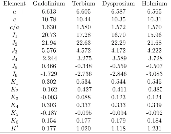
5.1 The table shows the pair ({Jn}) and quartic ({Kn},K0) constants in
meV/f.u. units obtained from the fitting of the SDFT-DLM data of Gd with the lattice attributes of Gd, Tb, Dy, and Ho. These have been scaled by the de Gennes factor. The lattice parameters used in the calculation in atomic units are also shown. . . 77 5.2 Application of the theory to Tb, Dy and Ho. The values ofTN,Ttand
theT of the highestHof the dis-HAFM phase (T1andH1in Fig. 5.2)
are compared to experiment. Theoretical estimate of the tricritical point (A) is also given. Gd has a PM-to-FM second-order transition atTC=274K (TC=293K in experiment [1]). We remark that the HRE
metals Er and Tm, which have larger lanthanide contractions, form incommensurate HAFM structures at lowT and show no transitions to FM states [1], in agreement with the trends predicted here. . . 82 6.1 The eigenvectors (Vp,1(q = 0), Vp,2(q = 0), Vp,3(q = 0)) associated
to ˜up(q=0) = max(˜ui(q=0)) for the same compressive and tensile
strains shown in Fig. 6.4. The components correspond to the three Mn atoms in the PM unit cell illustrated in Fig. 6.1(a). In particular,
Vp,1 and Vp,2 are linked to the atomic positions (0 0.5 0.5) and (0.5 0
0.5), andVp,3 to (0.5 0.5 0), in lattice parameter units. . . 97
List of Figures
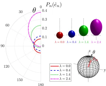
3.1 The dependence of the single-site probability Pn(ˆen) on the polar
angleθ(degrees), defined with respect to the orientation ofλn=βhn
(parallel to the z-axis), for four characteristic values of λn = |λn|.
The figure shows that for increasing values of λn the shape ofPn(ˆen)
gradually changes from a sphere, in which all the directions in space are equally weighted, to an ellipsoid with ˆλn as the most preferable
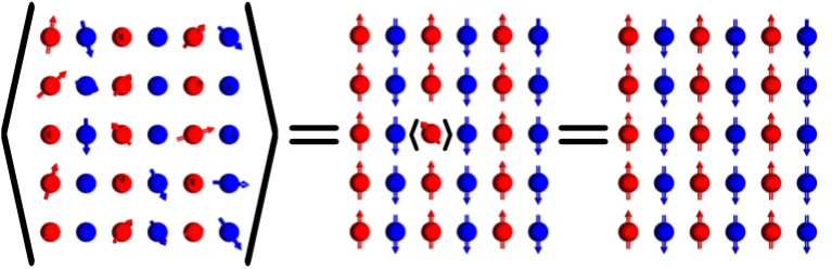
orientation. . . 34 3.2 The CPA of a two-dimensional system with two non-equivalent
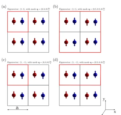
mag-netic positions (red and blue) whose fluctuating magmag-netic directions are oriented oppositely after the average is performed. The figure shows that when the red moment, for example, is surrounded by the effective medium, which is represented by the average orienta-tions, its fluctuation produces in average the same scattering effects as the effective medium itself. The same condition has to be fulfilled by the blue local moment so that the resulting effective medium is constructed from the CPA prescription at every magnetic site self-consistently. . . 41 3.3 The figure shows four different high temperature magnetic structures
of an arbitrary system with two non-equivalent magnetic positions (Nat = 2), denoted with red and blue, and the corresponding
eigen-vectors and values of q. The magnetic unit cell is indicated with colour red. Note that for the system be ferromagnetic it is neces-sary that q=0 and the components of the eigenvector are parallel, as shown in panel (a). We also remark that arrows in this figure represent the local order parameters{mn}. . . 50
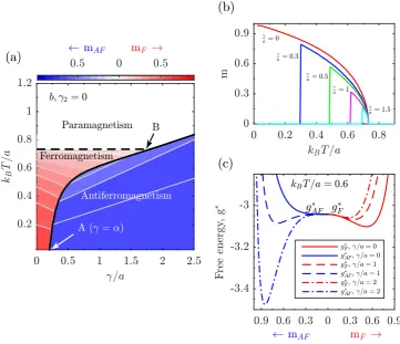
4.1 (a) The temperature - b/a phase diagram. Dashed and continuous black lines indicate second- and first- order transitions, respectively. (b)magainst temperature for pertinent values of the model parame-ters above and below the critical point. (c,d,e) The free energy below, at, and above the transition temperature for relevant model parame-ters, showing the difference between second- and first- order transitions. 62
−m2 in blue when gF∗ > gAF∗ . Dashed and continuous black lines
indicate second- and first- order transitions, respectively. (b) The total order parameter normalised inside the unit cell, m = (m1 +
m2)/2, for increasing values ofγ/a. (c) The free energiesg∗F (red and
right side) and gAF∗ (blue and left side) for pertinent values of γ/a
illustrating the first- order behaviour. . . 63
4.3 The lattice Fourier transform of the direct correlation function, ˜Ss=1s0=1(q) =
˜
uP(q), against the wave vectorqat the paramagnetic state. The
fig-ure shows two characteristic directions of q along (0 0 1) and (1 1 0). . . 65
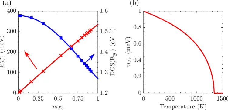
4.4 (a) The fieldhintF e(blue squares) and the density of states at the Fermi energy (red crosses) against the ferromagnetic order parametermF e.
Straight lines are the fitting functions of these quantities. (b) The temperature dependence of the local order parameter. . . 65
5.1 (a) Ferromagnetic, (b) fan, and (c) helical antiferromagnetic mag-netic phases observed in the heavy rare earth elements, illustrated by a ten- ferromagnetic layer scheme with single-site magnetisations perpendicular to the c axis. Colours blue and red are used to dis-tinguish between the two non-equivalent atomic positions inside one crystallographic unit cell of the hexagonal close packed structure. . . 71
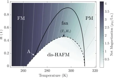
5.2 The generic magnetic T-H phase diagram for a heavy lanthanide metal for H applied along the easy direction constructed from the-ory. Continuous (discontinuous) lines correspond to second- (first-) order phase transitions and a tricritical point is marked (‘A’). The cal-culations were performed for the prototype Gd with lattice constants appropriate to Dy. . . 73
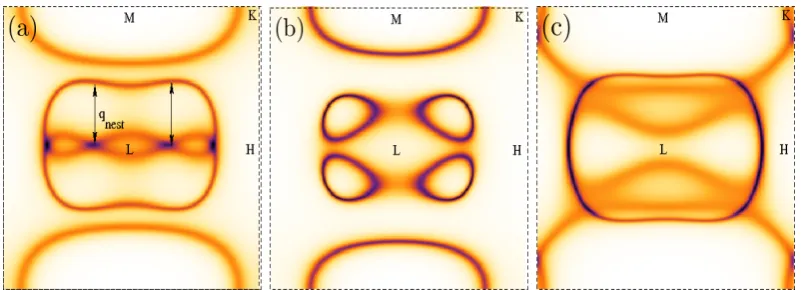
5.3 The Bloch spectral function A(k, E) in the LM HK plane at the Fermi energy for Gd with Dy’s lattice attributes for (a) the PM state and resolved into (b) majority spin and (c) minority spin com-ponents when there is an overall net average magnetisation of 54% (mFM = 0.54) of the T =0K saturation value in the FM state. This
is the value in our calculations (Fig. 5.2) in the FM phase just be-low the temperatureTtof the HAFM-FM first-order transition. qnest
indicates the nesting wave-vector of the FS of the PM state and the shading represents the broadening from thermally induced local mo-ment disorder. . . 75 5.4 The phase diagram of Gd with the lattice spacing of Dy when the
quartic coefficients are set to zero and the magnetic field is applied along the easy direction. Continuous (discontinuous) lines correspond to second- (first-) order transitions. . . 79 5.5 The phase diagram of Gd with the lattice spacing of Dy when the
magnetic field is applied along the hard direction. Continuous (dis-continuous) lines correspond to second- (first-) order transitions and a tricritical point is marked (A). . . 79 5.6 The lattice Fourier transform of the effective pair interactionsJeff(q)
(red line) whenmFM = 0 and its change when the FS is spin polarised,
for finitemFM (dashed blue line formFM= 0.3 and dot-dashed green
line for mFM = 0.54). The inset shows the dependence of the pair
interactions Jnn0 on separation x
nn0 =|xn−xn0|formFM=0. . . 81
5.7 The magnetic phase diagram constructed for Gd with the lattice at-tributes of (a) Gd, (b) Tb, (c) Dy, and (d) Ho. The de Gennes factor has been used to scale the quadratic and quartic coefficients (for the later we have used the square of the de Gennes factor) and the mag-netic field is applied along the easy direction. Continuous (discontin-uous) lines correspond to second- (first-) order phase transitions and a tricritical point (A) is marked when it exists. . . 83 5.8 The MCE quantified by (a) the isothermal entropy change and (b)
the adiabatic temperature change of Gd with the lattice attributes of Gd. The figure shows the results in the vicinity of the second-order PM-FM phase transition for increasing values of the applied magnetic field. . . 85
The figure shows the results in a temperature range comprising the PM-HAFM and HAFM-FM phase transitions for increasing values of the applied magnetic field. The appropriate de Gennes factor for Dy scaling the pair- and quartic constants has been applied. (c) Experimental isothermal entropy change from magnetisation data, taken from reference [2] for comparison with our results in panel (a). 86
6.1 (a) The antiperovskite paramagnetic (and also non-magnetic) unit cell of Mn3AX systems and the magnetic interactions between nearest
neighbours (red) and next nearest neighbours (blue). The element X sits on the cube centres and is surrounded by Mn atoms at the centre of the faces. The element A occupies the corner sites and can be one among many different elements or a solid solution of several (A=Ni, Ag, Zn, Ga, In, Al, Sn, etc.). The figure also shows some of the stable magnetic phases observed in experiment: The (b) ferromagnetic, (c) collinear antiferromagnetic (in Mn3GaC), and the triangular
antifer-romagnetic in the (d) Γ5g and (e) Γ4g representations [3]. Arrows
represent the averaged directions of the local magnetic moments and with colour blue we indicate the (111) plane. . . 90
6.2 Panel (a) shows the dependence of the maximum eigenvalue of the direct correlation function ˜Sss0(q) on the reciprocal wave vectorqfor
a lattice parameter minimising the SDFT-based total energya0=4.14
˚
A, which is plotted in panel (b). The results are shown for three char-acteristic directions from the centre to the boundaries of the Brillouin zone, red squares for (100), blues stars for (111), and green crosses for (101). The triangular state experimentally observed in Mn3GaN
6.3 The structure of Mn3GaN under compressive and tensile biaxial strains.
Magenta arrows are used to represent the induced canted angles and changes of the local order parameters and magnetic moment sizes. These changes as well as the tetragonal distortions are exaggerated for illustrative purposes. Red arrows show the unstrained magnetic structure for comparison. Upper and lower panels show the results at low and high temperatures, respectively: The (a,b) canted trian-gular state, and collinear (c) ferrimagnetic and (d) antiferromagnetic orderings. . . 95 6.4 The dependence of the largest value among {u˜i(q), i = 1,2,3} on
the reciprocal wave vector qalong the relevant direction (101). The results are shown for different values of (a) compressive (εxx <0) and
(b) tensile (εxx>0) biaxial strains. . . 96
6.5 The linear dependence of the quadratic constants a1, a2, α1, and
α2 obtained from fitting the SDFT-DLM data of {hintn } for εxx =
0,±0.25%,±0.50%,±1.00%. . . 98 6.6 Temperature-strain magnetic phase diagram of Mn3GaN. Colours
en-codes the size and orientation of the induced net magnetic moment,
µnet, along the (110) axis. Thick black lines indicate first-order (solid) and second-order (dashed) magnetic phase transitions. Letters in brackets link to panels of Fig. 6.3. . . 99 6.7 Total entropy of Mn3GaN against the temperature and biaxial strain.
Red contour lines mark adiabatic application of strain at Stot =
170 and 270 J/kgK. Black lines mark iso-strain cooling (εxx= 1.18%)
and heating (εxx =−0.73%). Blue isotherm marks the reference
tem-perature of 308 K and orange numbers indicate the proposed cooling cycle. . . 101 6.8 The total entropy for selected values of strain in Mn3GaN. Black
lines correspond to black iso-strain lines in Fig. 6.7 and blue dashed line crosses only the first-order phase transition (small ∆Tadmax
1 ). All
dash-dotted lines cross both the first- and second- order transitions allowing for larger ∆Tadmax
2 . . . 102
Firstly, I would like to express my deepest gratitude to my supervisor Prof. Julie B. Staunton, for her invaluable help and guidance, and for teaching me so much insightful knowledge in my travel through the world of magnetism. Her supervision has been beyond this project, she has been an extraordinary example of how to be an authentic researcher at both professional and human levels.
I am also thankful to Dr. Christopher Patrick for many inspiring and fruitful discussions and for absolutely always having time for my numerous questions.
A special mention to the great moments with ´Alvaro, Anna (el Rey), Anto, and Edoardo (la Reina): the funniest and most unproductive times of my PhD, and probably those where I have eaten more chocolate than ever. Siempre nos quedar´an los Chupa Chups de Pamplona!
My thoughts also go to Laura, Odette, and Samuele. Thank you very much for being such incredible friends and for so many hours of climbing and making an inside and outside of the office.
Finally, a heartfelt thank you to my family for their support and love, and especially to Sofia for being always with me. All the experiences we have lived together, although far from Warwick, have been unforgettable and are a treasure in my mind.
Declarations
This thesis is submitted to the University of Warwick as my application towards the degree of Doctor of Philosophy, and presents details of research carried out in the Theory Group of the Department of Physics between October 2014 and May 2018. The content of this thesis is my own work, unless stated otherwise, carried out under the supervision of Prof. J. B. Staunton. No part of this thesis has previously been submitted for a research degree at any other institution.
Parts of this thesis have been published in the following papers:
1. Chapter 5: Pair- and four- spin interactions in the heavy rare earth elements
• E. Mendive-Tapia and J. B. Staunton. Theory of magnetic ordering in the heavy rare earths: Ab initio electronic origin of pair- and four- spin interactions. Phys. Rev. Lett., 118:197202, 2017.
2. Chapter 6: Frustrated magnetism in Mn-based antiperovskite Mn3GaN
• J. Zemen, E. Mendive-Tapia, Z. Gercsi, R. Banerjee, J. B. Staunton, and K. G. Sandeman. Frustrated Magnetism and caloric effects in Mn-based antiperovskite nitrides: Ab initio theory. Phys. Rev. B,95:184438, 2017.
We present anab initio theory to describe magnetic ordering and magnetic phase transitions at finite temperatures from pairwise and multi-spin interactions. Our formalism is designed to model thermal fluctuations of disordered local mo-ments associated with atomic sites and adequately describes how these emerge from the glue of many interacting electrons. The key ingredient is to assume a time-scale separation between the evolution of the local moment orientations and a rapidly responsive electronic background setting them. This is the Disordered Local Mo-ment picture grounding the framework of our theory. The method uses Density Functional Theory calculations constrained to specific local moment configurations to model the electronic structure and exploits Green’s functions within a Multiple Scattering Theory to solve the Kohn-Sham equations. Two central objects are calcu-lated as functions of magnetic ordering: internal magnetic fields sustaining the local moments and the lattice Fourier transform of the interactions in the paramagnetic state. We develop a methodology to extract the pairwise and multi-spin constants from the first and use the second to study the magnetic interactions in the reciprocal space and gain information of the type and extent of most stable magnetic order. These quantities are directly related to the first and second derivatives of the free energy of a magnetic material, respectively. Hence, our approach is able to provide thermodynamic quantities of interest, such as temperature and entropy changes for the evaluation of caloric effects, and magnetic phase diagrams for temperature, mag-netic field, and lattice spacing studies can be constructed. Transition temperatures and their order, as well as tricritical points, are obtainable.
We apply the theory to carry out major investigations on long-period mag-netic phases in the heavy rare earth elements (HREs) and magmag-netic frustration in the Mn-based antiperovskite nitride Mn3GaN. The mixing of both pairwise and four-site
magnetic interactions have been found to have profound consequences on the mag-netism of both systems. We have obtained a generic HRE magnetic phase diagram which is consequent on the response of the common valence electronic structure to the f-electron magnetic moment ordering. We also present a modelling based on the lanthanide contraction to describe ferromagnetic, helical antiferromagnetic, and fan phases in Gd, Tb, Dy, and Ho, in excellent agreement with experiment. Our study of Mn3GaN shows that its first-order paramagnetic-antiferromagnetic
trian-gular transition originates from the fourth order terms and that the effect of biaxial strain to distort the compensated antiferromagnetic interactions has a large impact on the frustrated magnetism. As a consequence, new collinear magnetic phases sta-ble at high temperatures are predicted and a very rich temperature-strain phase diagram is obtained. We also show how to get the best refrigerating performance and design a novel elastocaloric cooling cycle from the features of the diagram.
Abbreviations
AFM Antiferromagnetic/antiferromagnetism ASA Atomic Sphere Approximation
BCE Barocaloric Effect bcc body centred cubic BZ Brillouin zone
CPA Coherent Potential Approximation DFT Density Functional Theory
dis-HAFM distorted helical antiferromagnetic/antiferromagnetism DLM Disordered Local Moment (theory)
DOS Density of states eCE Elastocaloric Effect ECE Electrocaloric Effect
FIM Ferrimagnetic/ferrimagnetism FM Ferromagnetic/ferromagnetism FS Fermi surface
HAFM Helical antiferromagnetic/antiferromagnetism hcp hexagonal close packed
HK Hohenberg-Kohn (theorem) HRE Heavy rare earth
KKR Korringa-Kohn-Rostoker (electronic structure method) LDA Local Density Approximation
LDA+U Local Density Approximation + U (Hubbard parameter) MCE Magnetocaloric Effect
MST Multiple Scattering Theory MTA Muffin-tin approximation PM Paramagnetic/paramagnetism
SDFT Spin- Density Functional Theory SIC Self-interaction correction SPO Scattering path operator TCE Toroidocaloric Effect
Chapter
1
Introduction
Magnetism is a collective phenomenon arising from the interactions among an im-mense number of particles. The mechanism of electrons travelling and mutually interacting with themselves and fixed nuclei in a magnetic material can result in the formation of ordered magnetic patterns, known as magnetic phases. The range of magnetic orderings observed in nature is enormous and rich. For example, the simplest situation corresponds to ferromagnetism in which magnetic moments, de-scribed by spin polarisation orientation of local electronic densities, are parallel aligned and a total non-zero magnetisation is produced. This order is in sharp con-trast with the magnetism originated in antiferromagnets, where the net magnetic moment vanishes due to the compensation of the local moment directions and sizes. As such condensed matter phases, the macroscopic behaviour of these magnetic structures is entirely distinct of their constituents and the whole is not described by the mere superposition of its parts. Understanding magnetism from an atomic point of view is a fundamental and exciting problem that due to its very compli-cated nature still today puzzles physicists even from what can be considered the most essential aspect: the description of the formation of the basic constituents, the magnetic moments, and in essence their nature. It should not be regarded as surprising that this basic task, in the sense of its elementary character, is yet not fully understood. Firstly, magnetic moments, whose collective behaviour de-termine macroscopic ordering, in turn emerge from the spins of many interacting electrons. This raises questions regarding the mutual influence between both co-operative mechanisms. Time and energy scale differences clearly play important roles in this mixing. Secondly, the spin of the electrons is a direct consequence of relativity, hence fundamentally including the complexity of relativistic effects into the intrinsic many-body quantum mechanical character. Finally, but not less
portant, empirical experience shows that relatively small temperature changes can have a profound impact on the properties of a magnetic material. For example, transitions between different kind of magnetic phases can be thermally triggered and warming up to high enough temperatures eventually destroys the magnetic or-dering without suppressing the magnetic moments themselves. Taking into account thermal fluctuations of local moments and their effect on the electronic glue, de-scribed by the sea of electrons binding together the nuclei, is a very complicated but essential task.
We present a theory to study the temperature-dependent magnetic proper-ties of materials from first principles, i.e. from a parameter-free formulation and relying on well established laws of nature only. Evidently, such a theory must be grounded in a sound quantum mechanical basis and ideally be fully extended to naturally include relativistic effects. Hence, we employ Density Functional Theory (DFT) [4, 5], a broadly used technique developed to solve the quantum mechani-cal equations of electrons in a solid within an effective single particle picture, thus designed to describe the electronic structure of a material. The choice of this mod-elling method is not made for its efficiency and versatility only, but also because it can be suitably implemented together with appropriate methods able to render magnetic disorder computationally tractable. The route to achieve this goes through the usage of Green’s functions and Multiple Scattering Theory (MST), known as the Korringa-Kohn-Rostoker (KKR)-MST method [6, 7], in honour to its early develop-ers. Such an approach distinguishes itself to other electronic structure techniques in that it uses the less intuitive Green’s functions as main mathematical tools, instead of the more familiar wave functions often employed in other DFT-based calculations. However, from this approach a rigorous formalism to describe thermally fluctuat-ing local magnetic moments affectfluctuat-ing and befluctuat-ing set by the underlyfluctuat-ing electronic structure can be established. The central tenet is to assume that the local moment orientations vary very slowly on the time-scale of the other electronic motions. This is the approach baptised as Disordered Local Moment (DLM) theory [8] and we entirely centre our treatment of magnetism at finite temperatures on such a pic-ture. DFT-DLM theory has been successfully implemented in the past and recent years to study, for example, the onset of magnetic order in strongly-correlated sys-tems [9] and the heavy rare earth elements [10], metamagnetic phase transitions in metal alloys [11, 12], the magnetic interactions between rare-earth and transition-metals [13, 14], and temperature-dependent magnetic anisotropy [15, 16, 17, 18].
em-3 braced by the DLM approach, and study their effect on magnetic phase transitions. Our theory is designed to model thermally induced excitations of the magnetic mo-ment orientations. It naturally describes how the spin-polarised electronic structure adapts to the extent and kind of magnetic order. As will be shown in chapter 3, a mean-field treatment is used to solve the statistical mechanics of the fluctuating disordered local moments, from which we develop a method to calculate pairwise and multi-spin interactions among them. We show how as the magnetic ordering develops at each atomic site the effect of multi-spin interactions might become im-portant in systems with a complicated coupling between the electronic glue and the local moments, which can be expected to occur in metallic magnets, for in-stance. The presence of these higher order terms, in principle, can have fundamental consequences on the magnetic behaviour when the amount and type of long-range magnetic order changes. Our method produces the free energy of the system as well as extent of magnetic orderings as functions of temperature, magnetic field and interatomic distances. It also describes temperature and entropy changes be-tween different magnetic states, hence being a natural tool for the calculation of caloric effects, which can be used to model magnetic materials for magnetic refriger-ation [19, 20]. We also develop a methodology to construct magnetic phase diagrams containing second- and first-order magnetic phase transitions and, therefore, locat-ing consequent tricritical points. Belocat-ing that the theory is able to track the order of the transitions, the examination of these diagrams can be used to predict previously unexplored phase-space regions with the most optimal conditions maximising ther-modynamical quantities of interest. As it will be shown, both pair- and multi-spin interactions, which in turn depend on the electronic structure behaviour, determine the phase diagram’s features.
phase diagrams. To demonstrate some of the particularities of the theory we apply it to bcc iron and present some simple case studies for illustrative purposes. Chap-ters 5 and 6 are dedicated to show new results. Respectively, we study in depth the incommensurate magnetism and temperature and magnetic field dependence of long-period magnetic phases, as well as ferromagnetism, in the heavy rare earth ele-ments, and the effect of biaxial strain on the frustrated magnetism in the Mn-based antiperovskite system Mn3GaN. These two chapters contain the original work
Chapter
2
Ab-initio
theory of electronic
structure
Describing the very complicated process of solid formation initially demands to fully solve the quantum many-body problem of coupled electrons and nuclei. This is a formidable task that must be simplified in order to be tractable. One can adopt the approach of designing a simpler Hamiltonian aimed to model a small number of degrees of freedom of interest, and let the rest to be captured by empirical parame-ters. This path fundamentally relies on experimental experience and adjusting the Hamiltonian to the specifications of each system is usually necessary. Alternatively, one refers toab initiomodelling, or equivalently a model from ’first principles’, when the theory used does not rely on empirical parameters and only free-parameter ap-proximations are incorporated. Such a theory is evidently very desirable and has been pursued in the last decades. Along these lines, the development of the well es-tablished Density Functional Theory (DFT) technique, which led to the Nobel prize in chemistry in 1998, represented a breakthrough since it provided the basis to study solids from purely theoretical inputs. DFT has been exploited to study very diverse phenomena and has substantially advanced the understanding in many fields, such as physics, chemistry, and engineering. Due to its reliability and relative simplicity it has become one of the most employed ab initio approaches and its study is an established field which is still continuously evolving yet today.
This chapter is devoted to introduce DFT, which will be used as theab initio
technique supporting our calculations describing the electronic structure. Firstly, in section 2.1 we derive the Kohn-Sham equations, present the approximation made for the calculation of the exchange and correlation functional, and show the formalism of DFT at non-zero temperatures. The formal solution of the Kohn-Sham equations,
based on the multiple scattering approach, is then presented and developed in section 2.2. Finally, in section 2.3 we introduce a theory to describe disorder by constructing an effective medium.
2.1
Density Functional Theory
DFT is aimed to make the very complicated problem of many interacting electrons surrounded by many nuclei tractable. The problem can be initially simplified by considering that in the solid state the nuclei typically remain at fixed positions, or barely move from them, compared with the fast travelling electrons. This is due to the fact that their mass is about three orders of magnitude larger than the mass of the electrons and, consequently, their electronic velocities must be much smaller. From this, one can neglect the kinetic energy of the nuclei and consider the effect of their presence as an external potential acting on the electrons. This is the so-called Born-Oppenheimer approximation [23]. In this situation the electrons feel the effect of a stationary effective field created by the slowly moving underlying nuclei arrangement and instantaneously adjust their motions to its evolution. The non-relativistic Hamiltonian operator describing this picture can be written as [24]
ˆ
H= ˆK+ ˆW +X
n
Vext(rn),
ˆ
K=− ~
2
2me
X
n
∇2r
n Wˆ =
1 2
X
n
X
m6=n
e2
4πε0|rn−rm|
,
(2.1)
whereε0 is the permittivity of vacuum ande,me, and rnare the charge, mass and
position of the n-th electron, respectively. The term labelled as ˆK is the kinetic energy, and the external potentialVextcomprises the effect of the fixed nuclei on the
electrons. The second term ˆW describes the Coulomb repulsion between electron pairs and, in practice, its presence makes the Hamiltonian in Eq. (2.1) too compli-cated to be solved as it stands, since it represents the source of the many-electron interaction. The strategy behind DFT to overcome this problem consists in convert-ing Eq. (2.1) into an independent electron Hamiltonian. This idea is implemented by firstly introducing the central concept of DFT established by Hohenberg and Kohn: the total energy of the system is a functional of the electron density n(r) only,
2.1. Density Functional Theory 7
n0(r) [4]. This observation simplifies the problem remarkably since it shows that
there is only need to find n(r), instead of the immense many-body wave function Ψ(r1,r2, . . .), in order to calculate the total energy at the ground state. Returning
now to Eq. (2.1), the total energy functional is expressed as
E[n] =hΨ[n]|Kˆ + ˆW|Ψ[n]i+ Z
drn(r)Vext(r) =F[n] +
Z
drn(r)Vext(r), (2.3)
where |Ψi is the many-body ground state wave function and F[n] = K[n] +W[n] is a universal functional which does not depend on the particularities of the crystal structure. The Kohn-Sham approach now follows by splittingF[n] into kineticK0,
and HartreeEH, energy terms of an effective independent electron system
reproduc-ing exactly the density of the original one,
F[n] =K0[n] +EH[n] +Exc[n]. (2.4)
Here
K0[n] =−~ 2
2m
X
i
Z
drψ∗i(r)∇2ψi(r)
EH[n] =
1 2
Z Z
drdr0n(r) e
2
4πε0|r−r0|
n(r0) = 1 2
Z
drn(r)VH(r)
(2.5)
defines the Hartree potential VH(r) and introduces the Kohn-Sham single-particle
wave functions{ψi(r)}, yet unknown, of the independent electron Hamiltonian. The
extra energy term Exc[n] in Eq. (2.4), named exchange and correlation energy, is
also unknown and accounts for the difference between the non-interacting effective medium and the many-body real system,
Exc[n] =K[n] +W[n]−K0[n]−EH[n]. (2.6)
In practice, this term has to be approximated and ideally it is expected to be rela-tively small. Evidently, the accuracy of DFT calculations largely rely on how this term is treated.
The electron density is computed from the single electron wave functions as
n(r) =X
i
|ψi(r)|2, (2.7)
uniquely the external potential of the nuclei Vext(r) [4, 5]. In fact this one-to-one
mapping does not depend on the explicit form of the electron-electron interaction and, in consequence, it guarantees the existence of a non-interacting system which has the same ground state electron density as the real system. In order to obtain the wave functions {ψn(r)}it is convenient to introduce the Lagrange functional
L[n] =E[n]−X
ij
λij[hψi(r)|ψj(r)i −δij], (2.8)
whereλij are the corresponding Lagrange multipliers ensuring the orthogonality of
the wave functions. The variational principle is then used to minimise the total en-ergy and simultaneously constrain the calculation to the correct number of electrons in the system,N. From Eq. (2.8) one then obtains
δL[n]
δn = 0⇒
δE[n]
δψi∗(r) − X
j
λijψj(r) = 0. (2.9)
After some simple algebra and using Eqs. (2.3), (2.4), and (2.5) one can write
−~
2∇2
2me
+Vext(r) +VH(r) +
δExc[n]
δn
ψi(r) =
X
j
λijψj(r), (2.10)
which can be rewritten in terms of rotated single-particle wave functions {φi(r)},
from diagonalizing λij, and the exchange and correlation potential is defined as
Vxc(r) =
δExc[n]
δn
n(r)
, (2.11) that is,
−~
2∇2
2me
+Vext(r) +VH(r) +Vxc(r)
φi(r) =εiφi(r), (2.12)
where {εi} are the single-particle energies. This set of equations are known as
the Kohn-Sham equations [5] and are the basis of DFT and the cornerstone of the most important modern computational electronic structure theories for modelling materialsab initio. Note that the effective potential finally derived in Eq. (2.12)
Veff(r) =Vext(r) +VH(r) +Vxc(r) (2.13)
depends on n(r) so that the Kohn-Sham equations can be solved self-consistently together with Eq. (2.7). An initial guess of the electron density is taken to calculate
2.1. Density Functional Theory 9 equations. At this point these solutions are used to recalculate the electron density. If one obtains a different value then a new guess is constructed and the cycle is repeated until self-consistency is reached. The total energy can be calculated too using the single-particle energies{εn}as
E[n] =X
i
fiεi−EH[n] +Exc[n]−
Z
drn(r)Vxc(r), (2.14)
wherefi = 1 (fi = 0) applies if the state is occupied (non-occupied) and the extra
terms are added to subtract double-counting terms in the Hartree and the exchange-correlation contributions.
2.1.1 The Local Density Approximation
As explained in the previous section, the exchange-correlation potential is designed to capture all the complicated many-body effects ignored within the independent electron approximation. Until today the corresponding electron density functional
Exc[n] is still unknown and continuous effort to construct accurate exchange and
correlation potentials constitutes an active research field itself. Here we employ the most common numerical scheme to approximateExc[n], the Local Density
Ap-proximation (LDA) [25, 26]. The idea is to calculate the exchange and correlation energies of a simpler system, the interacting homogeneous electron gas, and map them locally to the real medium. If the electron density is slowly varying, one can assume that Exc[n] in each infinitesimal volume element at a given position is the
same as the one calculated for the homogeneous electron gas with the same value of the charge density [24],
dExc =
Ehom xc [n(r)]
V dr⇒Exc[n] =
1
V
Z
drExchom[n(r)], (2.15) whereV is the volume andExc[n] is then obtained by adding up all the individual
contributions from each volume element. For the homogeneous electron gas the exchange functional can be derived exactly [27], while the correlation functional is extracted by solving numerically the many-particle Hamiltonian and parametrising the resulting data [25]. The total exchange-correlation functional is then obtained by summing up both contributions. In this thesis we implement the LDA and use the parametrisation proposed by Perdew and Wang [28].
universal functional. It is expected, therefore, that both the exchange and correla-tion effects are well described by the Coulomb repulsion and the quantum statistical nature included in the homogeneous electron gas.
2.1.2 Density Functional Theory extended to finite temperatures
Hohenberg and Kohn laid the basis of ab initio ground state calculations of elec-tronic structure. To accomplish this they demonstrated the existence of the universal functionalF[n], independent of the external potentialVext(r), such thatE[n] in Eq.
(2.3) is minimised for the ground state density n0(r) associated toVext(r) [4].
How-ever, the temperature effect on the population of excited electronic states was not considered. The extension of DFT to finite temperatures was realised by Mermin, soon after the publication of Hohenberg and Kohn, by following an analogous rea-soning in the context of the grand canonical ensemble [30]. The starting point is to construct the grand potential functional
Ω[ ˆρ] = Tr ˆρ
ˆ
H −νNˆ+ 1
βlog ˆρ
, (2.16) where ν is the chemical potential, ˆN is the particle number operator, and ˆH is the many-body Hamiltonian as expressed in Eq. (2.1). Eq. (2.16) naturally introduces the probability density operator ˆρ such that Tr [. . .] performs the trace operation and the expected value of an operator ˆA is calculated ashAˆi = Tr ˆρAˆ. The grand potential
Ω =−1
β log
Tr exp
h
−β( ˆH −νNˆ) i
(2.17) is given by Eq. (2.16) when ρ=ρ0 is the appropriate equilibrium density matrix
ρ0=
exph−β( ˆH −νNˆ)i Tr exph−β( ˆH −νNˆ)i
. (2.18)
The key point is that it is possible to show that in fact the minimum of Ω[ρ] is attained by ρ0 and, therefore, Vext(r) determines ρ0 [30]. Underlying the work of
Mermin is to show that the functional variable can be transferred from ρ to n(r) such that a universal functionalFT[n] independent ofVext(r) exists and that
Ω = Z
2.1. Density Functional Theory 11 is the grand potential too, i.e., it is minimised by the equilibrium density n0(r) in
the presence of Vext(r). Similarly to zero temperature DFT, it is straightforward
to show thatVext(r) is unequivocally determined byn0(r) byreductio ad absurdum
demonstration [30]. Since Vext(r) in turn determines ρ0, it can be deduced that ρ0
is a functional ofn0(r). From Eqs. (2.16) and (2.19), and recalling the Hamiltonian
in Eq. (2.1), it follows that
FT[n0] = Tr
ρ0[n0]
ˆ
K+ ˆW + 1
β logρ0[n0]
. (2.20) Eq. (2.19) is, therefore, the grand potential, showing that the approach presented by Hohenberg and Kohn can be implemented at non-zero temperatures.
In practice, the total energy expression given in Eq. (2.14) can be extended to non-zero temperatures by using the equilibrium electron density and the appropriate Fermi-Dirac occupation functionfn= 1 +eβ(εn−ν)
−1
to calculate Ω[n] = Ω0[n]−EH[n] + Ωxc[n]−
Z
drn(r)Vxc(r), (2.21)
where now the Hohenberg-Kohn energy functional becomes a Helmholtz free energy such that Ω0[n] → Pnfnεn −T S0 −νN, which can be described by the
non-interacting fermions entropy
S0 =−kB
X
n
h
fnlogfn+ (1−fn) log(1−fn)
i
. (2.22)
2.1.3 Magnetism and relativistic effects in Density Functional The-ory
The DFT approach presented in the previous sections does not depend on the spin since its presence has been ignored so far for simplicity. The concept of spin is a direct consequence of the extension of the Schr¨odinger equation to be invariant with respect to Lorentz transformations. In other words, it arises naturally in the framework of the Dirac equation. Similarly, the generalisation of DFT to take in magnetism goes through the consideration of special relativity effects. Pertinent to the spin inclusion, therefore, is to examine the Dirac equation for an electron moving under the effect of an external magnetic field specified by a vector potential, i.e. B=∇ ×A(r),
ˆ
HDΨi(r) =
h
cα·(−i~∇+eA(r)) +βImec2
i
Here c is the velocity of light and εi is the energy solution. βI is a four by four
matrix defined as
βI=
I2 (0)
(0) −I2
!
, where I2=
1 0 0 1
!
, (2.24) (0) being a matrix of zeros, and αis a vector whose components are defined as
α= (αx, αy, αz) with αi=
(0) σi
σi (0)
!
, (2.25) where {σi} are the well known Pauli matrices
σx=
0 1 1 0
!
, σy =
0 −i
i 0
!
, σz =
1 0 0 −1
!
. (2.26) The solution of Eq. (2.23), Ψi(r), is the famous Dirac spinor, which is structured
by four different components. Hence, it is natural to expect that in relativistic DFT the central role played by the electron density is replaced by a four-component function. Indeed, it has been shown that the total energy of the Dirac equation at the ground state is a unique functional of the relativistic four-component current
Jµ(r) [31]. This is not surprising as Jµ(r) conceals the electron density n(r) itself
as well as the spin density. It includes the electron current density too, although it is usually ignored if diamagnetism and electric polarisation effects are not the object of interest. If the starting point of the calculation is the Dirac equation and spin-polarisation effects are included we refer to Spin- Density Functional Theory (SDFT). Importantly, the extension to finite temperatures of SDFT can be carried out too by the same argument presented by Mermin [30] since the mapping of the probability density to Jµ(r) can be equivalently argued. As it is common practice,
in this thesis we focus our attention to the electron and spin densities only.
From energy comparison arguments and neglecting diamagnetism and or-bital paramagnetism, Eq. (2.23) can be safely approximated to the following two-component equation [24]
−~
2∇2
2me
+2µB
~ S ·B
Φi(r) =εiΦi(r). (2.27)
2.1. Density Functional Theory 13 by the spin operator
S= ~
2σ, where σ = (σx, σy, σz), (2.28) appears in the Dirac equation naturally. The Dirac spinor is now formed by inde-pendent two-spinor functions
Φi(r) =φi(r; 1)|↑i+φi(r; 2)|↓i , with |↑i=
1 0
!
and |↓i= 0 1
!
. (2.29) As usual, the electron density is constructed as the sum of the independent densities over occupied states
n(r) =X
i
ni(r) =
X
i
Φ†i(r)Φi(r) =
X
i
|φi(r; 1)|2+|φi(r; 2)|2
, (2.30)
such as the total number of electrons satisfiesNe=
R
drn(r). The total spin density is computed from the application of the spin operator,
s(r) =X
i
si(r) =
X
i
Φ†i(r)SΦi(r), (2.31)
which suggests the following definition of the associated total magnetic moment density
µ(r) =−2µB ~
X
i
si(r) =−
2µB
~ s(r). (2.32)
From the definition given in Eq. (2.28), together with Eq. (2.29), we can write after some simple algebra the dependence of the spin density on the Dirac solution,
sx(r) =~Re
X
i
φ∗i(r; 1)φi(r; 2)
, (2.33)
sy(r) =~Im
X
i
φ∗i(r; 1)φi(r; 2)
, (2.34)
sz(r) = ~
2 X
i
|φi(r; 1)|2− |φi(r; 2)|2
, (2.35)
which satisfies |s(r)| = ~
2n(r). An important observation regarding SDFT follows
non-trivial manner. Within this framework the total local magnetic moment per unit cell of volumeVu is obtained by performing the integral
µVu = Z
Vu
drµ(r). (2.36)
We return now to the density functional strategy of DFT and proceed to apply it to the Dirac equation. Clearly, once relativistic effects are included the first step is to consider the total energy as a functional of both the electron density and the magnetic moment density, i.e. E[n(r)] → E[n(r),µ(r)]. Adapting the Dirac equation to the approximations cementing DFT, namely the Born-Oppenheimer, mean-field (in the Hartree potential), and single-particle approximations, the total energy can be expressed in terms of the kinetic, exchange-correlation, and Hartree energies already introduced for non-relativistic DFT, as well as an extra contribution accounting for the external magnetic field
E[n,µ] =K0[n,µ] +EH[n,µ] +Exc[n,µ] +
Z
drn(r)Vext(r)−B·µ(r)
. (2.37) The SDFT Kohn-Sham equations are then derived by following an analogous min-imisation procedure with respect to n(r) and µ(r), as described in section 2.1. For this purpose we define the density matrix
nαβ(r) =
X
i
φ∗i(r;α)φi(r;β), (2.38)
which compactly contains both densities,
n(r) =X
α
nαα(r) and µ(r) =−µB
X
αβ
nαβ(r)σαβ. (2.39)
The minimum principle follows, therefore, as
δE[nαβ]
δnαβ
= 0, (2.40) which, together with the use of the Lagrange parameter associated with the particle number conservation, leads to the SDFT version of the Kohn-Sham equations
− ~
2
2me
∇2+Vext(r) +VH(r) +Vxc(r)−µBσ·(B(r) +Bxc(r))
Φi(r) =εiΦi(r),
2.2. Multiple Scattering Theory 15 where
δExc[nαβ]
δnαβ
n(r),µ(r)
=Vxc(r)I2+µBσ·Bxc(r). (2.42)
This equation shows that the very complicated many-electron physics, captured by the exchange-correlation energy, might generate an effective magnetic field Bxc(r)
at every point in space. Evidently, this term comprises the effect of Pauli exclu-sion principle and the Coulomb interaction fundamentally behind magnetism and in principle captured by the LDA. It is this term, therefore, the one that is responsible of magnetic ordering if the appropriate conditions favouring the generation of spin polarisation are present.
The total energy can be calculated from Eq. (2.41) in analogy to the non-relativistic computation shown in Eq. (2.14),
E[n,µ] =X
i
fiεi−EH[n] +Exc[n,µ]−
Z
drn(r)Vxc(r)−
Z
drµ(r)·(B(r) +Bxc(r))
(2.43) Note that the main difference is that a term accounting for the contribution of the total magnetic field is added.
2.2
Multiple Scattering Theory
that single-site scattering events can be solved independently of the geometry of the system so that the problem can be conveniently separated into two parts.
In practice, The KKR-MST formalism and mechanism is exactly the same for both relativistic and non-relativistic approaches. The main difference lies in that the size of the central quantities, such as the Green’s functions and scattering ma-trices, which become higher within the relativistic formulation due to the additional spin-dimensionality. The shapes of the spherical expansions, solving the scattering problems, are consequently different too, but the central equations and relations defining the theory remain the same. For this reason, we present in the following pages the non-relativistic derivation for illustrative purposes and to avoid the math-ematical complication added in the relativistic picture. This is appropriate since the relevant non-relativistic results can then be healed to incorporate relativistic effects by suitably tracing with respect to the spin degrees. The interested reader can find detailed derivations of the relativistic formulation in many references, such as [34, 35, 36, 37].
2.2.1 Green’s functions and the single-center scattering problem
In this section the Green’s function formulation is presented and used to solve the problem of one particle being scattered by a single localised potential. The results obtained will become the basis to expand the theory to deal with a collection of scattering potentials in section 2.2.2.
We proceed by recalling the effective potential derived in Eq. (2.13). Our starting point is to approximate it as a sum of non-overlapping spherical potentials centred at fixed positions{Rn},
Veff(r)≈
X
n
Vn(rn), with rn=r−Rn, (2.44)
where rn = |rn|, and Vn(rn) = 0 for rn > rMT,n, rMT,n being named the
muffin-tin radius of the spherical region n. Note that rMT,n can be different at each site.
This form to split Veff(r) is known as the muffin-tin approximation (MTA) and the
region of zero potential outside the spheres is referred to as the interstitial region. Many authors use, additionally, other manners to approximateVeff(r). For example,
2.2. Multiple Scattering Theory 17 principle the ASA should be treated carefully if applied.
In this picture the Kohn-Sham Hamiltonian ˆHKS = −~2∇2/2me+Veff(r)
is meant to describe a particle travelling across an ensemble of scattering centres that are associated to the potentials created at each site of the lattice system. The solution of the single-centre scattering event at siten, which we denote withϕn(r),
is described by the single-site Hamiltonian equation ˆ
Hn(r)ϕn(r) =
−~
2∇2
2me
+Vn(rn)
ϕn(r) =Eϕn(r). (2.45)
From this equation the Green’s function associated to ˆHn(r) is formally defined as
Gn(E) = lim →±0
E−Hˆn+i−1, (2.46) whose real space representation version satisfies
(E−Hˆn(r))Gn(r,r0, E) =δ(r−r0). (2.47)
Similarly, the free-particle Green’s function G0(r,r0, E) is defined by replacing ˆHn
by the free-particle Hamiltonian ˆH0(r) = −~2∇2/2m
e in Eq. (2.45). The
advan-tage of using Green’s functions is that the free-particle trajectory can be connected to the scattered solution. For example, the well known Dyson equation expresses
Gn(r,r0, E) in terms ofG0(r,r0, E) as [34],
Gn(r,r0, E) =G0(r,r0, E) +
Z
dr00G0(r,r00, E)Vn(r00−Rn)Gn(r00,r, E)
=G0(r,r0, E) +
Z Z
dr00dr2G0(r,r00, E)tn(r00,r02, E)G0(r2,r0, E).
(2.48)
The previous expression defines the real space representation of the very useful
t-matrix function, tn(r,r0, E). It is this quantity the one that we are interested
to calculate since it fully describes the scattering effect from a single potential. Importantly, it satisfies a similar version of the Dyson equation itself1
tn(r,r0, E) =Vn(rn)δ(r−r0) +
Z
dr1Vn(rn)G0(r,r1, E)tn(r1,r0, E). (2.49)
In addition, the scattered wave function is connected to the free electron solution
φn(r) by
ϕn(r) =φn(r) +
Z
dr0G0(r,r0, E)Vn(r0−Rn)ϕ(r0)
=φn(r) +
Z Z
dr0dr00G0(r,r0, E)tn(r0,r00, E)φn(r00),
(2.50)
which is the so-called Lippmann-Schwinger equation. We point out that both this relation and the Dyson equation for the t-matrix can be shown by applying the operator (E−Hˆ0(r)) in both sides of the equations themselves. The way to proceed now is to note that in the interstitial region of constant potential the wave function can be expressed in terms of plane waves. This allows to exploit the spherical symmetry of the problem by writingφn(r) as the following expansion
φn(r)→exp (ik·r) = 4π
X
L
iljl(kr)YL∗(ˆr)YL(ˆk), (2.51)
where the sum is over the pair of quantum numbers L = (l, m), YL(ˆr) are the
corresponding spherical harmonics2, andj
l(kr) is the spherical Bessel function [36].
The single-particle Green’s function can be expanded as a linear combination of spherical harmonics and Bessel functions too [36],
G0(r,r0, E) =−
exp (ik|r−r0|)
4π|r−r0| =−ik
X
L
jl(kr<)h+l (kr>)YL(ˆr)YL∗(ˆr0). (2.52)
Here r> = max{r, r0},r< = min{r, r0}, and h+l (kr>) are the spherical Hankel
func-tions. Introducing Eqs. (2.51) and (2.52) into Eq. (2.50) and setting rn > rMT,n
gives
ϕn(r) = 4π
X
L
ilYL∗(ˆk) "
jl(kr)YL(ˆr)−ik
X
L0
h+l0(kr)YL0(ˆr)tn,L0L(E)
#
, (2.53) which defines the t-matrix in the angular momentum representation
tn,L0L(E) =
Z Z
drdr0jl0(kr0)YL∗0(ˆr0)tn(r0,r, E)jl(kr)YL(ˆr). (2.54)
The solution presented in Eq. (2.53) is regular at the origin (|rn| → 0) due to the
good behaviour of the spherical Bessel functions employed. A different definition of regular solutions is commonly used too, which are in general known as the scattering
2
They satisfy ˆL2YL(ˆr) =l(l+1)YL(ˆr) and ˆLzYL(ˆr) =mYL(ˆr), where ˆLis the angular momentum
2.2. Multiple Scattering Theory 19 solutions,
Zn,L(r, E) =
X
L0
jl0(kr)YL0(ˆr)t−1
n,L0L(E)−ikh+l (kr)YL(ˆr), with rn> rMT,n. (2.55)
In principle, irregular solutions should be included to fully describe the wave function too [36]. They are typically chosen as [36]
Hn,L(r, E) =−ikh+l (kr)YL(ˆr). (2.56)
These solutions must be matched to the form inside the bounding sphere, which can be obtained from Eq. (2.50) at rn < rMT,n. Alternatively the differential form
expressed in Eq. (2.45) can be used too, leading to the usual radial equation reflecting the spherical symmetry of the system. This operation determines thet-matrix and, therefore, yields the single-site problem solved. For computational purposes the angular momentum sums must be truncated at some maximum value. For most of the typical calculations withlmax = 3 give satisfactory results in terms of accuracy
and at the same time yield computational affordable costs.
Finally, the single-site Green’s function can be also obtained from the scat-tering solutions as [34, 36]
Gn(r,r0, E) =
X
LL0
Zn,L(r, E)tn,LL0(E)Z×
n,L0(r, E)−
X
L
Zn,L(r<, E)Jn,L× (r>, E),
(2.57) where the superscript× applies the conjugate operation on the spherical harmonics and Jn,L(r, E) = Rn,L(r, E)−ikh+l (kr)YL(ˆr), Rn,L(r, E) being the radial part of
the wave solution.
2.2.2 Scattering paths and the multi-site solution
The central idea of the MTA is to approximate the effective potential as a collec-tion of non-overlapping single-centre scatterers. This construccollec-tion has a remarkable consequence in the context of MST: the solution of the Kohn-Sham Hamiltonian, composed by the single-site potentials
ˆ
HKS(r) = ˆH0(r) +
X
n
Vn(rn), (2.58)
potential. Keeping ˆH0 as the non-perturbed reference system, the corresponding
Dyson equation is structured from every single-centre potential as well as the free-particle Green’s function. This leads to the generalisation of Eq. (2.49) as
T =X
n
Vn+X
n
VnG0T . (2.59) We have switched to the angular momentum representation, which naturally yields matrix equations with angular momentum labels. Henceforth underlined quantities are used to represent their angular momentum matrix form, following the definition given in Eq. (2.53). For example, the components ofVnare
Vn,LL0(E) =
Z Z
drdr0jl0(kr0)YL∗0(ˆr0)Vn(r−Rn)δ(r−r0)jl(kr)YL(ˆr). (2.60)
Eq. (2.59) defines the T-matrix in terms of itself. We can now expand the right hand side of this equation and expressT as a sum involving the single-site potentials and G0. Note that now G0 connects potentials that are centred at different fixed positions. To continue exploiting the spherical symmetry of each scattering event, we expand G0 around two different centre positions. After carrying out the algebra one obtains [36]
G0,nm,LL0(E) =−4πik
X
L1
il−l0−l1CL1
LL0YL1( ˆRnm)h +
l1(Rnm, E), (2.61)
where Rnm=Rm−Rn,Rnm=|Rnm|, and the constants
CL1 LL0 =
Z
dˆrYL(ˆr)YL∗0(ˆr)YL1(ˆr) (2.62)
are known as the Gaunt numbers. By repeating substitution ofT into Eq. (2.59), and using the Dyson equation of thet-matrix in the angular momentum representation (tn=Vn+VnG0tn), one can finally write the central multiple scattering equation
T =X
n
Vn+X
nm
VnG0,nmVm+X
nmk
VnG0,nmVmG0,mkVk+. . .
=X
nm
h
tnδnm+tnG0,nm(1−δnm)tm+. . .
i
.
2.2. Multiple Scattering Theory 21 Hence, T depends on the matrices {tn} and G0,mn, as we were seeking to show. From this result we can introduce the scattering path operator (SPO),τmn,
T =X
mn
τmn⇒τmn=tnδnm+tn
X
k
G0,nk(1−δnk)τkm. (2.64)
The SPO gives a useful physical interpretation of the multiple scattering theory presented here. By inspecting the effect of applying the operator G0τmn on the incoming free-electron plane wave, and recalling the Lippman-Schwinger equation, it is clear that the SPO sums the effect of all scattering paths beginning at site
n and finishing at site m. The T-matrix then comprises every possible scattering event in the entire solid. The limitation of Eq. (2.63), as stated at the beginning of the section, is that the potentials must not overlap. This is manifest by recalling that the t-matrices are obtained by matching the spherical solutions to the free-particle plane wave at the muffin-tin radii. Overlapping potentials break down this spatial pattern so that the calculation would be inconsistent. In addition to this, as pointed out in Refs. [33, 35], the form given in Eq. (2.61) should not be used at the superposed regions, which yields the real space version of Eq. (2.63) intractable for overlapping potentials.
A more convenient expression for the SPO can be directly obtained by ma-nipulating Eq. (2.64). The following objects whose components are matrices in the angular momentum representation must be defined first,
τ(E) ={τnm}, t(E) ={tnδnm}, G0(E) ={(1−δnm)G0,nm}. (2.65)
Introducing this into Eq. (2.64) gives
τ(E) =t−1(E)−G0(E)
−1
. (2.66) This is another central equation that will show itself as very useful in future deriva-tions and manipuladeriva-tions.
To conclude this section, we finally show an expression for the full Green’s function associated with the multiple scattering problem. By using the scattering solutions and the corresponding Dyson equation one can finally write [36]
G(r,r0, E) =Zn(r−Rn, E)τnm(E)Z×m(r0−Rm, E)
−δnmZn(r<−Rn, E)J×n(r>−Rn, E),
(2.67)
mo-mentum indices. The index n (m) in the right hand side is chosen such that the vector r (r0) is inside the respective spherical potential. The KKR-MST strategy is clear now. The SPO is constructed via application of Eq. (2.66). It is composed by thet-matrices containing all atomic-like information and the scatterer connector
G0,nm, which is determined separately by the geometry of the system. Once this
result is obtained theT-matrix and the Green’s function can be directly calculated from Eqs. (2.64) and (2.67), respectively.
2.2.3 Density calculation and the Lloyd formula
This section is devoted to show how to use G(r,r0, E) to obtain the electron and magnetic moment densities. We start by expressing the formal definition of the Green’s function given in Eq. (2.47) in terms of the eigenvalues and eigenfunctions of the Hamiltonian of interest. Naming these quantities{Ei}and{ψi(r)}for ˆHKS(r),
respectively, one can write
G±(r,r0, E) = lim
→±0
X
i
ψi(r)ψ∗i(r0)
E−Ei+i
=X
i
ψi(r)ψi∗(r0)
P 1
E−Ei
∓iπδ(E−Ei)
,
(2.68) where P stands for the Cauchy principal value. By recalling Eq. (2.39), it directly follows that
n(r) =∓1
πImTr
Z
dEf(E)G±(r,r, E), (2.69) where f(E) is the appropriate occupation function and Tr[. . .] traces over spin coordinates for the two-spinor Dirac solution in SDFT if necessary. Similarly, the magnetic moment density is
µ(r) =±µB
1
πImTr
Z
dEf(E)βIΣG±(r,r, E), (2.70)
where
βIΣ=βI
σ (0)
(0) σ
!
= σ (0) (0) −σ
!
. (2.71) The density of states at energy E can be provided by the Green’s function too after performing similar manipulations
n(E)≡X
i
δ(E−Ei) =∓
1
πImTr
Z
drG±(r,r, E) =∓1
πImTrG
±(E). (2.72)
2.3. The effective medium theory of disorder: the Coherent Potential
Approximation 23
equality. The total number of electrons is then
N =
Z ∞
−∞
dEf(E)n(E) =∓1
πImTr
Z ∞
−∞
dEf(E) Z
drG±(r,r, E), (2.73) which becomes
N(EF) =N0(EF) +δN(EF), (2.74)
with
N0(EF) =±
1
πImTr logG ±
0(EF), (2.75)
δN(EF) =±
1
πImTr logT ±(E
F), (2.76)
whenf(E) adopts the shape of the Fermi-Dirac function in the limit of approaching zero temperature, i.e. f(E < EF) = 1 andf(E > EF) = 0, forEF being the Fermi
energy. The serviceable Dyson equation as well as some identities of the Green’s function and theT-matrix have been used to arrive to Eqs. (2.75) and (2.76) [36], which are known as the famous Lloyd formula.
2.3
The effective medium theory of disorder: the
Co-herent Potential Approximation
and co-authors that the CPA was expressed in terms of the SPO in the angular momentum representation for a muffin-tin approximated potential, hence yielding a numerically tractable scheme [33, 39].
The CPA consists in replacing the disordered crystal potential by an effective ordered medium that forces the electrons to adopt the average behaviour as closely as possible [33, 38, 39, 40, 41]. The key idea that made the CPA successful com-pared with its rival alternative, the averaged t-matrix approximation (ATA) [42], was that the CPA is shaped as a self-consistent approach. While in the ATA the effective potential is chosen beforehand, usually following the virtual crystal model, in the CPA it plays the role of a parameter that is found by satisfying some more sophisticated criterion. By testing the predictions of both approximations the CPA has been shown to give more accurate results compared with the ATA. In fact, the CPA is usually referred to as the best possible single-site approximation [40].
The CPA condition is that the scattering occurring if the disordered site is embedded by the effective medium is exactly the same as the generated if the site is filled by the effective medium itself. Returning to scattering theory language, the effective medium is mapped to the so-called coherent potential,Vc(r) =PnVn(|r−
Rn|), constructed with a muffin-tin shape, as defined in Eq. (2.44). As usual, the
Dyson equation can be invoked to write the central scattering quantities at each site of the coherent lattice in the angular momentum representation,
Gc,n=G0+G0tc,nG0, (2.77)
⇒ tc,n=Vc,n+Vc,nG0tc,n. (2.78) HereG0is the Green’s function of the free-particle, andGc,nandtc,nare the Green’s function and t-matrix associated with the coherent potential at siten, respectively. Let’s assume now that the disorder at a chosen site n0 is determined by a
combi-nation of different single-site potentials {Vα,n0(|r−Rn0|)}, enumerated by α and
with probability Pα,n0 to randomly exist at the site
3. The effect of replacing the
muffin-tin sphere of the coherent potential by Vα,n0(|r−Rn0|) at site n0 can be
described by
Gα,n0 =Gc,n0 +Gc,n0tdiffα,n0Gc,n0, (2.79) wheretdiffα,n0 is not the appropriatet-matrix ofVα,n0(|r−Rn0|), but one that accounts
for the difference between this and the coherent potential, that is
tdiffα,n0 = Vα,n0−Vc,n0
+ Vα,n0 −Vc,n0
Gc,n0tdiffα,n0. (2.80)
3Evidently, the probabilities are restricted to satisfyP
2.3. The effective medium theory of disorder: the Coherent Potential
Approximation 25
Clearly, from these relations the CPA condition can be translated to the scattering terminology as
X
α
Pα,n0t diff
α,n0 = 0, (2.81)
which evidences the single-site nature of the approximation. Note that this equation can be expressed in terms of Green’s functions from Eq. (2.79) as
Gc,n0 =X
α
Pα,n0Gα,n0. (2.82)
In order to make the CPA implementable, it is desirable to write Eq. (2.81) in terms of the SPO. To this end, we consider separately each impurity problem with probabilityPα,n0, i.e. a lattice where the coherent potential is present at every site
apart fromn0, which is filled by Vα,n0(rn0). If we write Tα(n0) as the appropriate
multiple scattering T-matrix in this situation, the Dyson equation for the total Green’s function is
Gα(n0) =G0+G0Tα(n0)G0, (2.83) where the subscript (n0) is added to indicate the site of the impurity. This expression
together with Eqs. (2.81) and (2.82) allows to connect{Tα(n0)}to the total scattering
T-matrix of the coherent potential lattice Tc as
Tc=X
α
Pα,n0Tα(n0), (2.84)
which in turn may be written in terms of the SPO by making use of Eq. (2.64) [33],
τc,n0n0 =X
α
Pα,n0τα(n0),n0n0. (2.85)
The last two expressions show that the effective medium can be also understood as a fictitious system that produces a multiple scattering effect that is equal to the corresponding average at the site, when it is indeed surrounded by the coherent medium itself. The CPA is, therefore, referred to as the mean-field approximation in scattering theory. We point out that Eq. (2.85) has been able to be spatially resolved thanks to the fact that the switch to the angular momentum representation can be conveniently realised for non-overlapping muffin-tin spheres [33]. Moreover, a solution for the impurity SPO can be obtained by recalling Eq. (2.66). Considering the (n0, n0)-component of this equation only gives
τ−c,n10n0 =τ−α(n1
0),n0n0 −t
−1
α(n0),n0 +t
−1
where nowt−α(n1
0),n0 is the appropriatet-matrix at the disordered site of the impurity
problem. After some trivial manipulation of Eq. (2.86) one can write [39]
τα(n0),n0n0 =Dα,n0τc,n0n0, (2.87) where
Dα,n0 =h1 +t−α(n1
0),n0 −t
−1 c,n0
τc,n0n0i−1 (2.88) is the so-called impurity matrix. Similarly, one can define the following object, known as the excess scattering matrix,
Xα,n0 =
t−α(n1
0),n0 −t
−1 c,n0
−1
+τc,n0n0
−1
, (2.89) which satisfies
τα(n0),n0n0 =τc,n0n0 +τc,n0n0Xα,n0τc,n0n0, (2.90) sinceDα,n0 = 1 +τc,n0n0Xα,n0. From Eq. (2.87) the CPA prescription given in Eq. (2.85) can be conveniently expressed as
X
α
Pα,n0Dα,n0 = 1, (2.91)
or alternatively as
X
α
Pα,n0Xα,n0 = 0, (2.92)
and the CPA can be finally numerically implemented by solving these equations self-consistently. The approach presented here allows to obtain {t−c,n10} and τc,n0n0
from {t−α(n1
0),n0}, which are the quantities naturally calculated from the scattering