Multi-Temporal Depth Motion Maps-Based Local
Binary Patterns for 3D Human Action Recognition
Chen Chen,
Member, IEEE,
Mengyuan Liu,
Student Member, IEEE,
Hong Liu,
Member, IEEE,
Baochang Zhang,
Member, IEEE,
Jungong Han,
Member, IEEE,
and Nasser Kehtarnavaz,
Fellow, IEEE
Abstract—This paper presents a local spatio-temporal
descrip-tor for action recognition from depth video sequences which is capable of distinguishing similar actions as well as coping with different speeds of actions. This descriptor is based on three processing stages. In the first stage, the shape and motion cues are captured from a weighted depth sequence by temporally overlapped depth segments, leading to three improved depth motion maps (DMMs) compared to previously introduced DMMs. In the second stage, the improved DMMs are partitioned into dense patches, from which the local binary patterns histogram features are extracted to characterize local rotation invariant texture information. In the final stage, a Fisher kernel is used for generating a compact feature representation, which is then combined with a kernel-based extreme learning machine (ELM) classifier. The developed solution is applied to five public do-main datasets and is extensively evaluated. The results obtained demonstrate the effectiveness of this solution as compared to the existing approaches.
Index Terms—Action Recognition, Depth Motion Maps, ELM
Classifier, Local Binary Patterns, Fisher Kernel.
I. INTRODUCTION
A
CTION recognition plays a significant role in a number of computer vision applications such as context-based video retrieval, human-computer interaction and intelligent surveillance systems [1], [2], [3], [4], [5]. Many previous works have focused on recognizing actions captured by con-ventional RGB video cameras, e.g., [6], [7]. However, these works have limitations such as coping with various lighting conditions and cluttered backgrounds due to the fact that RGB data suffer from these variations, thus impeding effectiveness in real-world applications, such as video surveillance.More recent advances have involved performing action recognition by exploiting depth cameras. Compared with RGB cameras, depth cameras have several advantages: 1) depth data are much more tolerant to changes in lighting conditions and depth cameras even work in dark environments; 2) color and texture do not appear in depth images, which makes the tasks of human detection and foreground extraction from cluttered
C. Chen is with Center for Research in Computer Vision, University of Cen-tral Florida, Orlando, Florida, USA (e-mail: [email protected]).
M. Liu and H. Liu are with Shenzhen Graduate School, Peking University, Beijing 100871, China (e-mail: [email protected], [email protected]).
B. Zhang is with Beihang University, Beijing 100080, China (e-mail: [email protected]).
J. Han is with School of Computing and Communications, Lancaster University, Lancaster, LA1 4YW, UK (e-mail: [email protected]).
N. Kehtarnavaz is with Department of Electrical Engineering, University of Texas at Dallas, Richardson, TX 75080, USA (e-mail: [email protected]).
[image:1.612.323.553.187.320.2]H. Liu is the corresponding author.
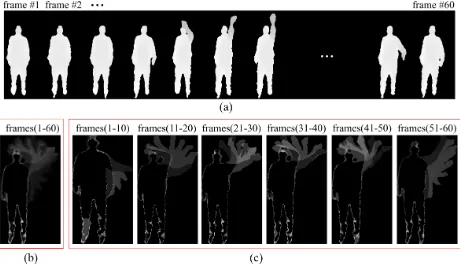
Figure 1. An example of different levels of DMMs representations.
backgrounds easier [8]; 3) depth cameras provide depth im-ages, which capture the 3D structural data of subjects/objects in the scene [9]; 4) human skeleton positions (e.g., 3D joints positions and rotation angles) can be efficiently obtained from depth images providing additional information for performing action recognition [10].
Since the release of cost-effective depth cameras, such as Microsoft Kinect, many works on action recognition have been conducted using depth images. Various representations of depth sequences have been explored, including bag of 3D points [11], spatio-temporal depth cuboid [12], depth motion maps (DMMs) [13], [14], [15], [16], surface normals [17], [8] and skeleton joints [18]. Among these representation schemes, DMMs-based representations transform the action recognition problem from 3D to 2D and have been successfully applied to depth-based action recognition. Specifically, DMMs are obtained by projecting the depth frames onto three orthogonal Cartesian planes and accumulating the difference between projected maps over an entire sequence. They are basically used to describe the shape and motion cues of a depth action sequence.
frames (e.g., frames 1-10, 11-20, 21-30, etc.) in the same action sequence. It can be observed that the detailed motion (e.g., raising hand over head and waving) of a hand waving action can be observed in DMMs generated using subsets of depth frames in a depth action sequence. In other words, the waving motion exhibited in the DMMs generated from subsets of depth frames is more obvious and clear than that in the DMMs generated using the entire depth sequence (all frames). In addition, action speed variations may result in large intra-class variations in DMMs. To overcome the above shortcomings of DMM representations, a new local spatio-temporal descriptor is developed by taking into consideration the shape discrimination and action speed variations. The contributions of this work are as follows:
• The original DMM representation is improved by non-linearly accumulating weighted motion regions of a sequence onto three orthogonal Cartesian planes. By doing so, the temporal relationships among frames are retained. In addition, to cope with speed variations in actions, different temporal lengths of depth segments are employed, eventually leading to a multi-temporal DMM representation.
• A set of local patch descriptors are built by partitioning all the DMMs into dense patches and utilize the local binary patterns (LBP) [19] to characterize local rotation invariant texture information in those patches.
• To make the representation more compact, the Fisher kernel [20] is used to encode the patch descriptors, which is fed into a kernel-based extreme learning machine (ELM) classifier [21] for recognition.
A preliminary version of the above approach appeared in [22]. This paper extends that work in the following manner. First, a more comprehensive survey on related works is pro-vided. Second, an improved set of DMMs is proposed based on a nonlinear weighting function to assign different weights to depth frames, thereby preserving the temporal information among different frames. Third, the method developed in this paper has been evaluated on four benchmark datasets and a comprehensive comparison is provided with the state-of-the-art approaches including deep learning methods, e.g., [23]. The experimental results show that our method outperforms these existing methods. Fourth, an MSRAction3D-Speed dataset has been put together based on the original MSRAction3D dataset [11], which is used to demonstrate the robustness of our method to speed variations. It is worth noting that our method is flexible in the sense that it can be combined with skeleton joints employing a similar multi-temporal structure.
The remainder of this paper is organized as follows. Section 2 briefly reviews related works. Section 3 provides the details of our proposed depth video representation method. The ex-perimental results on several benchmark datasets are reported in Section 4. Finally, Section 5 concludes the paper.
II. RELATEDWORK
As pointed out in [24], 3D action recognition methods can be categorized into three types: depth-based, skeleton-based, and depth-skeleton-based methods. This section reviews these three types of methods briefly.
Surface normal vectors [25] can reflect local structure of 3D objects, therefore they are widely used for 3D object retrieval. An extended version called Histogram of Oriented 4D Normal vectors (HON4D) [17] is developed to capture local structure of spatio-temporal depth data. The 4D space denotes time, depth and 2D spatial coordinates. Since HON4D captures local information of one point separately, Histogram of Oriented Principal Components (HOPC) [26] is proposed to capture relationships surrounding that point. Specifically, HON4D cal-culates principal directions within a volume around the point and then encodes three main principal directions. Compare with HON4D, HOPC is more robust to depth noise, due to the usage of principal directions. Moreover, HOPC is able to capture relationships among local points. However, HOPC ignores relationships among points in a large scale. To solve this problem, a depth sequence is treated as many pairwise 3D points, and the relative depth relationships are used to construct binary descriptors [27]. This representation captures both local and global relationships. An alternative solution appears in [28], where a depth sequence is split into spatio-temporal cells, and then a locality-constrained linear coding is applied to encode features extracted from these cells. Despite of above methods, many types of descriptors are developed. For example, 2D and 3D auto-correlation of gradients features are combined using a weighted fusion framework for action recognition [29]. In [30], a tensor subspace, whose dimension is learned automatically by low-rank learning, is developed for RGB-D action recognition. Recent works on depth-based 3D action recognition focus more on specific problems such as cross-view action recognition. In [31], a depth video based cross-view action recognition method is developed, which learns a general view-invariant human pose model from syn-thetic depth images using a convolutional neural network and a sparse Fourier Temporal Pyramid to encode action specific features for spatio-temporal representation.
between body parts. In [18], the 3D geometric relationships among human body parts are explicitly modeled as curves using a Lie group. With the progress of deep learning [35], recent works use a single image to encode spatio-temporal information of skeleton joints, and then fine-tune pre-defined models for transfer learning. In [23], the skeleton is divided into five parts, which are used as inputs for five bidirectional recurrent neural networks (BRNNs). Then, the representations from the subnets are fused in a hierarchical way to be the inputs to higher layers. Since recurrent neural network (RNN) can model the long-term contextual information of temporal sequences, the proposed end-to-end hierarchical RNN achieves high performances on the task of skeleton-based action recog-nition. In [36], a skeleton sequence is visualized as several color images, which explicitly encode both spatial distributions and temporal evolutions of skeleton joints. To enhance the discriminative power of color images, skeleton joints with salient motions are emphasized when generating these color images. Finally, enhanced color images are used as inputs for a multi-stream convolutional neural networks, which explores the complementary properties between color images. Although combining deep learning methods and some hand-crafted fea-tures can obtain high recognition performance, skeleton-based methods are not applicable for applications where skeleton information is not available.
When skeleton joints can be stably estimated, these joints reflect robust motion patterns of human actions, thereby avoid-ing the effect of noisy depth data. However, in human-object interaction scenarios, skeleton joints can barely capture any information about the object. Moreover, when the human body is not directly facing the depth sensor, the estimated skeleton joints are usually noisy. In these cases, original depth data provides essential cues for distinguishing similar actions. In the direction of depth and skeleton information fusion, an ensemble model [37] is proposed to associate local occupancy pattern features from depth images with skeleton joints. In this way, the object can be reflected by describing depth data surrounding skeleton joints. Moreover, traditional HOG feature is also used to describe depth data surrounding skeleton joints [38]. Although multi-modal fusion methods generally achieve higher recognition accuracy, having a depth descriptor on top of a complicated skeleton tracker makes such algorithms computationally expensive, limiting their use in real-time applications.
III. PROPOSEDDEPTHVIDEOREPRESENTATION A. Improved Depth Motion Maps
According to [14], the DMMs of a depth sequence withN
frames are computed as follows:
DM M{f,s,t}=
N
X
i=2
|mapi{f,s,t}−map{i−f,s,t1 }|, (1)
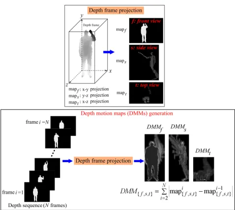
[image:3.612.318.557.51.264.2]where mapif,mapis andmapit indicate three projected maps of the ith depth frame on three orthogonal Cartesian planes corresponding to the front view (f), side view (s) and top view (t). A graphical illustration of DMMs generation is presented in Fig. 2.
Figure 2. DMMs generation for a depth sequence.
On each orthogonal Cartesian plane, the DMMs are for-mulated by accumulating projected maps through an entire sequence. In this case, the temporal relationships among frames are not taken into consideration. To accommodate for the temporal relationships, an improved version of DMMs is provided here.
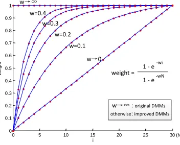
In order to describe the motion in RGB video, in [39] Motion Energy Image (MEI) was considered, which contains the motion information through accumulating binary processed image frames. To preserve the temporal information between different frames, in [39] a linear weighting function was considered with the time as an independent variable. After assigning each frame a weight, a Motion History Image (MHI) was generated, where more recently moving pixels are brighter. An analogy to this approach is adopted here between DMMs and MEI, and an improved DMMs is thus developed that follows a similar design flow of MHI. Different from the linear weighting function in [39], a nonlinear weighting function is designed which facilitates the weighting scheme. By adjusting one parameter, one would be able to obtain a set of weighting functions, which incorporates the linear weighting function.
Specifically, our weight in the weighting function is defined as follows:
weight(i) = 1−e
−wi
1−e−wN, (2)
where i indicates the ith frame in a sequence with N total
frames and the parameterwcontrols the shape of the weight-ing function. Accordweight-ingly, the improved DMMs is defined as:
DM M{f,s,t}=
N
X
i=2
|mapi{f,s,t}−mapi{−f,s,t1 }| ∗weight(i),
0 5 10 15 20 25 30 0
0.1 0.2 0.3 0.4 0.5 0.6 0.7 0.8 0.9 1
t
w
e
ig
h
t w→0
w→∞
w=0.1 w=0.4
w=0.3 w=0.2
(N)
w→∞ : original DMMs otherwise: improved DMMs
1 - e-wi weight =
1 - e-wN
[image:4.612.400.476.56.136.2]i
Figure 3. A weighting function for constructing improved DMMs. An action sequence withN= 30frames is illustrated for example.
and the improved DMMs becomes the original DMMs. When
w → 0, the weighting function becomes a linear function, which is similar to the weighting scheme in [39].
B. Multi-temporal Depth Motion Maps
As aforementioned, DMMs based on an entire depth se-quence may not be able to capture detailed motion cues. To capture more motion information, a depth sequence is divided into a set of overlapped 3D depth segments with equal number of frames (i.e., same frame length for each depth segment) and three DMMs are computed for each depth segment. Since different people may perform an action at different speeds, multiple frame lengths are also used to represent multiple tem-poral resolutions to cope with speed variations. The proposed multi-temporal DMMs representation framework is shown in Fig. 4. This figure illustrates an example where DMMs are generated by using the entire depth sequence (i.e., all the frames in the sequence) is considered to be the default level of the temporal resolution (denoted by Level 0 in Fig. 4). In the second level (Level 1 in Fig. 4), the frame length (L1) of
a depth segment is set to 5 (i.e., 5 frames in a depth segment). In the third level (Level 2 in Fig. 4), the frame length (L2)
of a depth segment is set to 10. Note that L1 andL2 can be
changed. Obviously, the computational complexity increases by increasing temporal levels. Thus, the maximum number of levels is limited here to 3 including the default level, i.e., Level 0, which considers all the frames. The frame interval (R,R < L1 andR < L2) in Fig. 4 is the number of frames
between the first frames (or the starting frames), respectively, in two neighboring depth segments, indicating the amount of overlap between the two segments. For simplicity, the sameR
in Level 1 and Level 2 is used here.
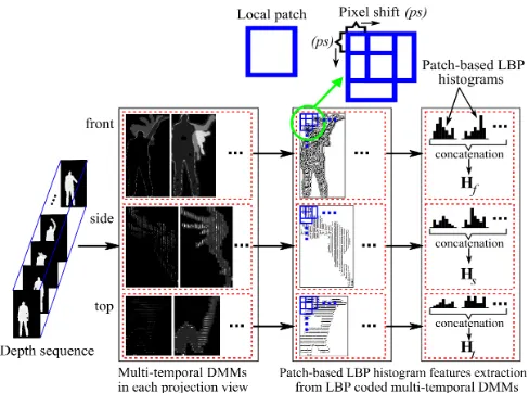
C. Patch-based LBP Features
DMMs can effectively capture the shape and motion cues of a depth sequence. However, DMMs are pixel-level features. To enhance the discriminative power of DMMs, the patch-based LBP feature extraction approach in [15] is adopted here to characterize the rich texture information (e.g., edges, contours, etc.) in the LBP encoded DMMs.
g1
g3
g4
g2
π/2 r gc
Figure 5. Center pixelgcand its 4 circular neighbors{gi}3i=0with radius
rfor the LBP operator.
The LBP operator [19] is a simple yet effective gray scale and rotation invariant texture operator that has been used in various applications. It labels pixels in an image with decimal numbers that encode local texture information. Given a pixel (scalar value)gc in an image, its neighbor set contains pixels
that are equally spaced on a circle of radius r (r > 0) with the center at gc. If the coordinates of gc are (0,0) and m
neighbors {gi}mi=0−1 are considered, the coordinates of gi are
(−rsin(2πi/m), rcos(2πi/m)). The gray values of circular neighbors that do not fall in the image grids are estimated by bilinear interpolation [19]. Fig. 5 illustrates an example of a neighbor set for(m= 4, r= 1)(the values for mandrmay change in practice). The LBP is created by thresholding the neighbors{gi}mi=0−1 with the center pixelgc to generate am
-bit binary number. The resulting LBP forgc can be expressed
in decimal form as follows:
LBPm,r(gc) = m−1
X
i=0
U(gi−gc)2i, (4)
where U(gi −gc) = 1 if gi ≥ gc and U(gi−gc) = 0 if gi < gc. Although the LBP operator in Eq. (4) produces 2m
different binary patterns, a subset of these patterns, named uniform patterns, is thus able to describe image texture [19]. After obtaining the LBP codes for pixels in an image, an occurrence histogram is computed over an image or a region to represent the texture information.
Fig. 6 shows the process of patch-based LBP feature extraction. The overlap between two patches is controlled by the pixel shift (ps) illustrated in Fig. 6. Under each projection view, a set of patch-based LBP histogram features are generated to describe the corresponding multi-temporal DMMs. Therefore, three feature matricesHf,HsandHtare
generated which are associated with front view DMMs, side view DMMs and top view DMMs, respectively. Each column of the feature matrix (e.g., Hf) denotes a histogram feature
vector of a local patch.
D. A Fisher Kernel Representation
Fisher kernel representation [20] is an effective patch aggre-gation mechanism to characterize a set of low-level features, which shows superior performance over the popular Bag-of-Visual-Words (BoVW) model. Therefore, the Fisher kernel is employed here to build a compact and descriptive representa-tion of the patch-based LBP features.
[image:4.612.85.261.63.205.2]Figure 4. Proposed multi-temporal DMMs representation of a depth sequence.
Figure 6. Patch-based LBP feature extraction.
the multi-temporal DMMs of a particular projection view (e.g., front veiw) for a depth sequence. By assuming statistical independence,Hcan be modeled by aK-component Gaussian mixture model (GMM):
p(H|θ) =
M
Y
i=1 K
X
k=1
ωkN(hi|µk,Σk), (5)
where θ = {ωk,µk,Σk}, k = 1, ..., K is the parameter set
with mixing parametersωk, meansµkand diagonal covariance
matricesΣkwith the variance vectorσk2. These GMM
param-eters can be estimated by using the Expectation-Maximization (EM) algorithm based on a training dataset (or feature set).
Two D-dimensional gradients with respect to the mean vector µk and standard deviation σk of the kth Gaussian
component are defined as
ρk =
1 M√πk
M
X
i=1
γk,i
hi−µk σk
,
τk =
1 M√2πk
M
X
i=1
γk,i
hi−µk σk
2
−1
!
,
(6)
where γk,i is the posterior probability that qi belongs to
the kth Gaussian component. The Fisher vector (FV) of H is represented as Φ(H) = (ρT
1,τ1T, ...,ρTK,τ T K)
T, where Φ
denotes the FV encoding operator. The dimensionality of the FV is2KD.
A power-normalization [20], i.e., signed square rooting (SSR) and`2normalization, is applied to eliminate the
sparse-ness of the FV as follows:
sgn(Φ(H))|Φ(H)|α, 0< α≤1. (7)
The normalized FV is then denoted byf.
Given NT training action sequences with NT
fea-ture matrices from a projection view v ∈ {f, s, t},
{H[1]v ,H[2]v , ...,H[vNT]}representing patch-based LBP
descrip-tors from multi-temporal DMMs are obtained using the feature extraction method demonstrated in Fig. 6. For each projection view v, the corresponding feature matrices of the training data are used to estimate the GMM parameters via the EM algorithm. Therefore, for three projection views, three GMMs are created. After estimating the GMM parameters, three FVs (ff, fs and ft) are generated for a depth sequence. Then,
the three FVs are simply concatenated as the final feature representationfcon= [ff;fs;ft]. Fig. 7 shows the steps toward
generating FVs.
[image:5.612.53.297.324.505.2]Figure 7. FV representation.
in ELM are randomly generated leading to a much faster learning rate. Compared with ELM, KELM provides a better generalization performance and is more stable. Therefore, this paper uses KELM for classification.
IV. EXPERIMENTS
To evaluate our approach, we report the outcome of our method on five datasets. The comparison between our method and related works are used to demonstrate the effect of multi-temporal DMM and LBP descriptor. In Section F, we report the time cost of our method and show the effect of levels on our multi-temporal structure. In Section G, we select proper parameter for the improved DMM and compare its performance with DMM.
A. MSRAction3D dataset
[image:6.612.50.301.53.253.2]1) Dataset: MSRAction3D dataset[11] is one of the most popular depth datasets for action recognition as reported in the literature. It contains 20 actions: “high arm wave”, “horizontal arm wave”, “hammer”, “hand catch”, “forward punch”, “high throw”, “draw x”, “draw tick”, “draw circle”, “hand clap”, “two hand wave”, “sideboxing”, “bend”, “forward kick”, “side kick”, “jogging”, “tennis swing”, “tennis serve”, “golf swing”, “pick up & throw”. Each action is performed 2 or 3 times by 10 subjects facing the depth camera. It is a challenging dataset due to similarity of actions and large speed variations in actions. As shown in Fig. 8, actions such as “drawX” and “drawTick” are similar except for a slight difference in the movement of one hand. We have calculated the statistics for theMSRAction3Ddataset, which contains the actions executed by different subjects with different execution rates. To be more precise, the standard derivation of the sequence lengths (numbers of frames) across the actions is 9.21 frames (max: 13.30 frames; min: 4.86 frames), which means that execution rate difference is actually quite large.
Figure 8. Actions “drawTick” (left) and “drawX” (right) in theMSRAction3D
dataset.
2) settings: Following [11], the cross subject validation method was adopted here with subjects#1; 3; 5; 7; 9for train-ing and subjects #2; 4; 6; 8; 10 for testing. The kernel-based extreme learning machine (KELM) [21] was employed with a radial basis function (RBF) kernel as the classifier due to its general good classification performance and efficient compu-tation. In all the experiments, the parameters for KELM (RBF kernel parameters) were chosen as the ones that maximized the training accuracy by means of a 5-fold cross-validation test.
For our feature extraction, the DMMs of different action sequences were resized to have the same size for the purpose of reducing the intra-class variation. To have fixed sizes for
DM Mf, DM Ms and DM Mt, the sizes of these maps for
all the action samples in the dataset were found. Following our previous work in [15], the fixed size of each DMM was set to 1/2 of the mean value of all of the sizes. This made the sizes of DM Mf, DM Ms and DM Mt to be 102×54,
102×75 and 75×54, respectively. The block sizes of the DMMs were considered to be 25×27,25×25and25×27
corresponding toDM Mf,DM MsandDM Mt. The overlap
between two blocks was taken to be one half of the block size. This resulted in 21 blocks forDM Mf, 35 blocks forDM Ms
and 15 blocks forDM Mt.
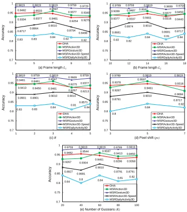
The same parameter values in [15] were used in our experimentations for the patch sizes and parameters for the LBP operator. The other parameters were determined empir-ically. The overall accuracies on three datasets with different parameters are shown in Figure 9, where frame length L1,
frame length L2, frame interval R, pixel shift ps and the
number of Gaussians (K) respectively change from 3 to 11, 10 to 18, 1 to 5, 3 to 7 and 20 to 100 at equal intervals. Experiments were conducted with one parameter changes and the other parameters were kept to the default values: L1= 7,
L2= 14,R= 3,ps= 5 andK= 60.
To build multi-temporal depth motion maps, a depth se-quence was divided into a set of overlapping 3D depth segments with equal number of frames. A three level structure of multi-temporal depth motion maps was considered, which needed three parameters, i.e.L1,L2andR. The frame lengths
of depth segments in the second and the third levels are respectively denoted by L1 and L2. These parameters were
determined by grid search from the grid[3,5,7,9,11]. Fig. 9 (a) and 9 (b) show the results under different values of L1
andL2. The overall trend is that the accuracy rises and then
falls with the increase ofL1 or L2. Small values ofL1 and
L2limited the depth information encoded in the depth motion
maps. While large values reduced the discriminative power of the 3D depth segments among different levels.
0.9482 0.9503 0.9461 0.9254 0.9275 0.9304 0.9377 0.9597 0.9377 0.9340 0.9819 0.9819 0.9819 0.9759 0.9729
0.8717
0.8864 0.9010
0.8754 0.8498
0.83 0.83 0.84 0.82
0.82 0.7 0.75 0.8 0.85 0.9 0.95 1
3 5 7 9 11
DHA MSRAction3D MSRGesture3D MSRAction3D-Speed MSRDailyActivity3D Ac c uracy
(a) Frame length L1
0.9399
0.9337 0.9461 0.9316 0.9440 0.9377
0.9487 0.9597
0.9377 0.9450 0.9789 0.9759 0.9819 0.9699 0.9759
0.8681
0.8974 0.9010
0.8681 0.8717
0.83 0.82 0.84
0.81 0.84 0.7 0.75 0.8 0.85 0.9 0.95 1
10 12 14 16 18
DHA MSRAction3D MSRGesture3D MSRAction3D-Speed MSRDailyActivity3D Ac c uracy
(b) Frame length L2
0.9461 0.9461 0.9461 0.9275 0.9213 0.9413 0.9450 0.9597 0.9267 0.9377 0.9819 0.9759 0.9819
0.9669 0.9759
0.8901 0.8901 0.9010 0.9010 0.8571
0.83 0.83 0.84
0.81 0.84 0.7 0.75 0.8 0.85 0.9 0.95 1
1 2 3 4 5
DHA MSRAction3D MSRGesture3D MSRAction3D-Speed MSRDailyActivity3D Ac c uracy
(c) R
0.9378 0.9461 0.9316 0.9267 0.9597 0.9084
0.9789 0.9819 0.9819
0.8791 0.9010 0.8717 0.8 0.84 0.82 0.7 0.75 0.8 0.85 0.9 0.95 1
3 5 7
DHA MSRAction3D MSRGesture3D MSRAction3D-Speed MSRDailyActivity3D Ac c uracy
(d) Pixel shift (ps)
0.9482 0.9544 0.9461 0.9296 0.9358 0.9267 0.9304 0.9597 0.9413 0.9450 0.9759 0.9819 0.9819 0.9789 0.9819
0.8827 0.8681
0.9010
0.8791 0.8791
0.84 0.8 0.84
0.81 0.82 0.7 0.75 0.8 0.85 0.9 0.95 1
20 40 60 80 100
DHA MSRAction3D MSRGesture3D MSRAction3D-Speed MSRDailyActivity3D Ac c uracy
[image:7.612.105.478.55.478.2](e) Number of Gussians (K)
Figure 9. Recognition accuracies with changing parameters.
Fig. 9 (c) shows the results with different values of R. Small value ofRled to a dense sampling of 3D depth segments at the expense of a large amount of processing time. When the value of R was larger than the frame lengths of depth segments, many depth frames between neighboring depth segments were made discarded.
To describe DMMs by patch-based LBP features, the over-lap between two patches is controlled by the pixel shiftps. As shown in Fig. 9 (d), the performance was boosted when the number of ps was increased. The optimum value was found to be 5 for the number of ps. When pswas larger than this optimum value, the performances dropped. The reason is that the spatial relationships among patches become weak when the overlap rate becomes small.
The parameterKis used in our Fisher kernel representation. The value of K was set by grid searching from the grid
[20,40,60,80,100]. As shown in Fig. 9 (e), the best outcome on the four datasets with different values of K was obtained. Generally speaking, more than 90% accuracies with
dif-ferent parameters on three benchmark datasets was obtained, indicating the robustness of our method to parameter settings. The MSRAction3D-Speed dataset was more challenging than
MSRAction3Ddataset, since the execution rate difference was higher in our dataset by sampling a portion of frames from original sequences. Even so, more than 85% accuracy was achieved with different parameters on theMSRAction3D-Speed
dataset, again indicating the robustness of our method to speed changes. Since the default values of parameter L1, L2, R, ps
worked well for all the four datasets, the following experiments were conducted with these values as the default values. It was observed that proper values of K were needed for different datasets to achieve the best performance. In what is reported next, the value ofK was set to60for all the datasets.
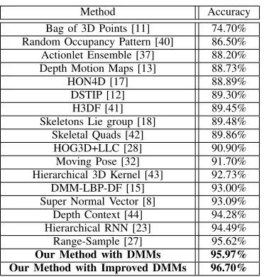
depth-Table I
RECOGNITION ACCURACY COMPARISON ON THEMSRAction3DDATASET.
Method Accuracy
Bag of 3D Points [11] 74.70% Random Occupancy Pattern [40] 86.50% Actionlet Ensemble [37] 88.20% Depth Motion Maps [13] 88.73%
HON4D [17] 88.89%
DSTIP [12] 89.30%
H3DF [41] 89.45%
Skeletons Lie group [18] 89.48% Skeletal Quads [42] 89.86%
HOG3D+LLC [28] 90.90%
Moving Pose [32] 91.70%
Hierarchical 3D Kernel [43] 92.73%
DMM-LBP-DF [15] 93.00%
Super Normal Vector [8] 93.09% Depth Context [44] 94.28% Hierarchical RNN [23] 94.49%
Range-Sample [27] 95.62%
Our Method with DMMs 95.97%
Our Method with Improved DMMs 96.70%
based features and “Actionlet Ensemble” [37] belongs to skeleton+depth-based features. Since only depth information is used in our method, no comparison could be done with the methods which use RGBD data.
“Moving Pose” [32] encodes 3D position, speed and ac-celeration of skeleton joints and achieves best performance among skeleton-based features. Despite the good performance of these methods, the skeleton data may not be reliable when the subject is not in an upright position. More over, the skele-ton data is not available from depth sequences which contains partial human bodies, e.g. hands, arms and legs. Therefore, the application areas of skeleton-based methods are limited. Our method outperforms these methods for two reasons: first, skeleton joints used by these methods contain a lot of noises, which bring ambiguities to distinguish similar actions; second, our method directly uses DMMs, thus providing more effective motion information.
“Range-Sample” [27] and “Super Normal Vector” [8] stand out from the depth-based features. In [27], the binary range-sample feature in depth is based on τ tests, which showed reasonable invariance to changes in scale, viewpoint and background. However, the temporal information among frames were not considered. In [8], an adaptive spatial-temporal pyramid based on the motion energy was proposed to globally capture the spatial and temporal orders. The dimension of action representation increased with the usage of larger num-ber of levels. In [8], three levels were used, which achieved limited performances. Our result is better than the recent depth-based features such as “Super Normal Vector” [8] and “Range-Sample” [27], demonstrating the superior discrimina-tory power of our multi-temporal DMMs representation.
[image:8.612.83.269.80.275.2]Using only patch-based LBP feature, DMM-LBP-DF [15] achieved an accuracy of 93.00%. Our Method with DMMs outperformed DMM-LBP-DF by nearly 3%, which verifies that multi-temporal DMMs can efficiently capture temporal information. Using improved DMMs instead of DMMs, our method allowed achieving the highest accuracy of 96.70%, indicating that the improved DMMs outperformed DMMs
Figure 10. Action snaps in theDHAdataset.
Table II
RECOGNITION ACCURACY COMPARISON ON THEDHADATASET.
Method Accuracy
D-STV/ASM [45] 86.80%
SDM-BSM [47] 89.50%
DMM-LBP-DF [15] 91.30%
D-DMHI-PHOG [48] 92.40%
DMPP-PHOG [48] 95.00%
Our Method with DMMs 95.44%
Our Method with Improved DMMs 96.27%
by preserving additional temporal information. It is noted that the performance of the improved DMMs depends on a parameter w. Therefore, a proper parameter value of w for different datasets needs to be selected as illustrated in Figure 14. More details about the comparison between DMMs and the improved DMMs are stated in Section IV-G.
B. DHA dataset
1) Dataset: DHA dataset is discussed in [45], whose action types are extended from the Weizmann dataset [46] which is widely used in action recognition from RGB sequences. It contains 23 action categories:“arm-curl”, “arm-swing”, “bend”, “front-box”, “front-clap”, “golf-swing”, “jack”, “jump”, “kick”, “leg-curl”, “leg-kick”, “one-hand-wave”, “pitch”, “pjump”, “rod-swing”, “run”, “skip”, “side”, “side-box”, “side-clap”, “tai-chi”, “two-hand-wave”, “walk”. Each action is performed by 21 subjects (12 males and 9 females), resulting in 483 depth sequences. In the DHA
dataset, “golf-swing” and “rod-swing” actions share similar motions by moving hands from one side up to the other side.
2) Settings: Similar to [48], the leave-one-subject-out eval-uation scheme was considered here, in which samples from one subject were chosen for testing and the remaining samples from the other subjects were used for training. Then, the overall accuracy was served as the evaluation criteria. The sizes of DMMs and blocks were set to the same values as the MSRAction3D dataset. All the other parameters were set to the default values.
Figure 11. Actions “milk” (left) and “hungry” (right) in theMSRGesture3D
dataset.
Table III
RECOGNITION ACCURACY COMPARISON ON THEMSRGesture3DDATASET.
Method Accuracy
Random Occupancy Pattern [40] 88.50%
HON4D [17] 92.45%
HOG3D+LLC [28] 94.10%
DMM-LBP-DF [15] 94.60%
Super Normal Vector [8] 94.74%
H3DF [41] 95.00%
Depth Gradients+RDF [49] 95.29% Hierarchical 3D Kernel [43] 95.66%
HOPC [26] 96.23%
Our Method with DMMs 98.19%
Our Method with Improved DMMs 99.39%
accuracy of86.80% on the original dataset. By incorporating the multi-temporal information to the DMMs, our method achieved higher accuracy even on the extended DHAdataset. From Table II, it can be seen that our method outperformed D-DMHI-PHOG [48] by3.04%and outperformed DMPP-PHOG [48] by 0.44%. These improvements show that operating LBP on multi-temporal DMMs can produce more informative features than operating PHOG on depth difference motion history images (D-MHI).
C. MSRGesture3D dataset
1) Dataset: MSRGesture3D dataset[40] is a benchmark dataset for depth-based hand gesture recognition. It consists of 12 gestures defined by American Sign Language: “bathroom”, “blue”, “finish”, “green”, “hungry”, “milk”, “past”, “pig”, “store”, “where”, “j”, “z”. Each action is performed 2 or 3 times by each subject, resulting in 336 depth sequences. Not that 333 depth sequences from MSRGesture3D dataset were used here and 3 sequences which contains no depth data were discarded. In theMSRGesture3Ddataset, actions such as “milk” and “hungry” are alike, since both actions involve the motion of bending palm.
2) Settings: Similar to [17], the leave-one-subject-out eval-uation scheme was employed and the overall accuracy was used to serve as the evaluation criteria. The sizes forDM Mf, DM MsandDM Mtwere118×133,118×29and29×133,
respectively. The block sizes of the DMMs were considered to be30×27,30×15and15×27corresponding toDM Mf, DM MsandDM Mt. All the other parameters were assigned
the default values.
3) Comparison with related works: In addition, a com-parison with several existing methods were conducted whose results appear in Table III. As can be seen from this table, our method outperformed Histogram of Oriented Principal Components (HOPC) [26] by 1.96%.
D. MSRAction3D-Speed dataset
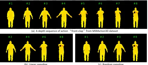
1) Dataset: MSRAction3D-Speed dataset is built using the MSRAction3D dataset. This dataset was used to test the
(a) A depth sequence of action “front-clap”from MSRAction3D dataset
(b) Linear sampling (c) Random sampling
# 1 # 2 # 3 # 4 # 5 # 6 # 7 # 8
# 2 # 4 # 6 # 8 # 1 # 2 # 3 # 8
Figure 12. Comparison between linear sampling method and random sampling method.
robustness of our method to frame rate difference. Specifically, the sequences performed by subjects 1, 3, 5, 7, 9, (the original action samples) were used as the training data. One half of the frames (odd number frames, e.g., 1, 3, 5 ...) of the sequences performed by subjects 2, 4, 6, 8, 10 were selected. Based on the original time order, the selected frames were concatenated to form new sequences. Two types of sampling methods were used for sampling frames, i.e. linear sampling and random sampling. The linear sampling method sampled frames with
1/2 of the original frame rate. While the random sampling method randomly sampled one half of the frames from the original sequences. As shown in Fig. 12, the random sampling-based MSRAction3D-Speed dataset was found to be more challenging than the linear sampling-based, since the speeds in the sampling-based dataset changed dramatically in a non-linear manner. Furthermore, many key frames got ignored by random sampling.
2) Settings: To facilitate a fair comparison with the results onMSRAction3Ddataset, the cross subject validation method was conducted with subjects #1; 3; 5; 7; 9 for training and subjects #2; 4; 6; 8; 10 for testing. All the other parameters were set to the same ones as used forMSRAction3D.
3) Comparison with related works: In view of the achieved
95.97% recognition rate on the MSRAction3D dataset, our method exhibited resistance to the execution rate. The achieved recognition result of our method on linear sampling-based
MSRAction3D-Speed dataset was 93.27%. Therefore, our method was capable of dealing with frame rate changes considering the fact that1/2frame rate reduction was actually unrealistic. The recognition result of our method on random sampling-based MSRAction3D-Speed dataset was 90.10%. Using only patch-based LBP feature, DMM-LBP-DF [15] achieved an accuracy of 83.88%. Our method outperformed DMM-LBP-DF by 6.22%, verifying that our multi-temporal structure can efficiently capture temporal information, coping with the effect of speed changes.
E. MSRDailyActivity3D dataset
overall accuracy (%) DHA MSRAction3D MSRGesture3D MSRAction3D‐Speed MSRDailyActivity3D
improved DMMs (w→0.0) 95.65 96.70 99.39 91.57 87
improved DMMs (w = 0.1) 95.65 96.34 99.39 90.10 88
improved DMMs (w = 0.2) 95.23 96.70 98.87 90.47 87
improved DMMs (w = 0.3) 96.27 95.97 99.20 90.47 88
improved DMMs (w = 0.4) 95.85 96.70 99.20 89.74 89
[image:10.612.48.299.190.270.2]original DMMs (w→∞) 95.44 95.97 98.19 90.10 84
Figure 14. Recognition accuracies with different parameterw.
drink eat call cellphone use vacuum cleaner cheer up
Toss paper lie down on sofa walk stand up sit down
Figure 13. Action snaps from theMSRDailyActivity3Ddataset.
in two different poses: “sitting on sofa” and “standing” by each subject, resulting in 320 depth sequences. This dataset contains cluttered backgrounds and noise. Moreover, most of the actions contain human-object interactions which are illustrated in Fig. 13.
2) Settings: Similar to [12], the sequences in which the subject was almost still were removed. As a result, our experiments were conducted with ten types of actions. A cross-subject validation was performed with cross-subjects 1,3,5,7,9 for training and subjects 2,4,6,8,10 for testing [50].
3) Comparison with related works: In Table IV, the com-parison of our method with related works on the MSRDaily-Activity3D dataset is provided. LOP feature [37] and Random Occupancy Pattern [40] are two typical features specially designed for encoding depth data. These methods achieved limited accuracies, which reflects the challenges (e.g. noise and cluttered backgrounds) of this dataset. To tackle with these challenges, DSTIP+DCSF [12] was recently designed, which achieves an accuracy of 83.60%. Our method achieved an improvement of2.4%over DSTIP+DCSF, since more depth data was captured by our multi-temporal depth motion maps. Actionlet Ensemble in [37] combines both depth data and skeleton data and achieves the state-of-the-art result of 86%. Without using skeleton data, our method is still competitive with Actionlet Ensemble. Since our method does not rely on the skeleton data, our method is more suitable for the real-world scenes, where the skeleton data can be barely captured (e.g. facing the problems of partial occlusions, viewpoint changes).
F. Computation Time
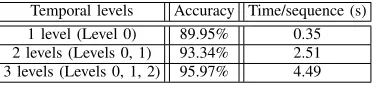
In our method, three levels for the multi-temporal DMMs representation is used. Our algorithm on the MSRAction3D
dataset was tested using different numbers of temporal levels. The recognition accuracy and average feature computation time are reported in Table V. It is worth mentioning that
Table IV
RECOGNITION ACCURACY COMPARISON ON THEMSRDAILYACTIVITY3D
DATASET.
Methods Accuracy
LOP feature [37] 42.50% STIPs (Harris3D+HOG3D) [51] 60.60% Random Occupancy Pattern [40] 64.00% Joint position feature [37] 68.00% STIPs (Cuboids+HOG/HOF) [52] 70.60%
DSTIP+DCSF [12] 83.60%
Actionlet Ensemble [37] 86.00%
Our Method with DMMs 84.00%
Our Method with Improved DMMs 89.00%
Table V
RECOGNITION ACCURACY AND AVERAGE FEATURE COMPUTATION TIME
OF OUR METHOD WITH DIFFERENT NUMBERS OF TEMPORAL LEVELS ON THEMSRAction3DDATASET.
Temporal levels Accuracy Time/sequence (s) 1 level (Level 0) 89.95% 0.35 2 levels (Levels 0, 1) 93.34% 2.51 3 levels (Levels 0, 1, 2) 95.97% 4.49
our algorithm is implemented in MATLAB and executed on CPU platform with an Intel(R)Core(TM)i7 CPU @2.60GHz and 8GB of RAM. The algorithm can be made more efficient by converting the code to C++ and running the multi-temporal DMMs representation in parallel.
G. Improved Depth Motion Maps
In Figure 14, our improved DMMs are compared with the original DMMs. To implement the improved DMMs, the parameter w was changed from 0 to 0.4 in 0.1 intervals. In practice, “w → 0” was implemented by setting w to
0.0001. It is noted that “w → 0” infers to apply a linear weighting function and that “w→ ∞” infers to directly apply the original DMMs, without using the weighing scheme. On
[image:10.612.345.532.384.427.2]Class 1 2 3 4 5 6 7 8 9 10 11 12 13 14 15 16 17 18 19 20 Recall(%)
highArmWave(1) 12 0 0 0 0 0 0 0 0 0 0 0 0 0 0 0 0 0 0 0 100
horizArmWave(2) 0 12 0 0 0 0 0 0 0 0 0 0 0 0 0 0 0 0 0 0 100
hammer(3) 0 0 12 0 0 0 0 0 0 0 0 0 0 0 0 0 0 0 0 0 100
handCatch(4) 0 0 0 9 0 1 0 1 0 0 0 0 0 0 1 0 0 0 0 0 75
forwardPunch(5) 0 0 0 0 11 0 0 0 0 0 0 0 0 0 0 0 0 0 0 0 100
highThrow(6) 0 0 0 0 0 11 0 0 0 0 0 0 0 0 0 0 0 0 0 0 100
drawX(7) 0 1 0 1 0 0 10 0 0 0 0 0 0 0 0 0 1 0 0 0 76.92
drawTick(8) 0 0 0 0 0 0 0 15 0 0 0 0 0 0 0 0 0 0 0 0 100
drawCircle(9) 0 1 0 0 0 0 0 1 13 0 0 0 0 0 0 0 0 0 0 0 86.67
handClap(10) 0 0 0 0 0 0 0 0 0 15 0 0 0 0 0 0 0 0 0 0 100
twoHandWave(11) 0 0 0 0 0 0 0 0 0 0 15 0 0 0 0 0 0 0 0 0 100
side-boxing(12) 0 0 0 0 0 0 0 0 0 0 0 15 0 0 0 0 0 0 0 0 100
bend(13) 0 0 0 0 0 0 0 0 0 0 0 0 15 0 0 0 0 0 0 0 100
forwardKick(14) 0 0 0 0 0 0 0 0 0 0 0 0 0 15 0 0 0 0 0 0 100
sideKick(15) 0 0 0 0 0 0 0 0 0 0 0 0 0 0 11 0 0 0 0 0 100
jogging(16) 0 0 0 0 0 0 0 0 0 0 0 0 0 0 0 15 0 0 0 0 100
tennisSwing(17) 0 0 0 0 0 0 0 0 0 0 0 0 0 0 0 0 15 0 0 0 100
tennisServe(18) 0 0 0 0 0 0 0 0 0 0 0 0 0 0 0 0 1 14 0 0 93.33
golfSwing(19) 0 0 0 0 0 0 0 0 0 0 0 0 0 0 0 0 0 0 15 0 100
pickup&throw(20) 0 0 0 0 0 0 0 0 0 0 0 0 0 0 0 0 0 0 0 14 100
[image:11.612.54.562.55.192.2]Precision(%) 100 85.71 100 90 100 91.67 100 88.24 100 100 100 100 100 100 91.67 100 88.24 100 100 100 96.70%
Figure 15. Confusion matrice of our method with improved DMMs on theMSRAction3Ddataset. The number in red indicates the overall accuracy.
Class 1 2 3 4 5 6 7 8 9 10 11 12 13 14 15 16 17 18 19 20 21 22 23 Recall(%)
arm-curl(1) 20 0 0 0 0 0 0 0 0 0 0 0 0 0 0 0 0 0 0 0 0 1 0 95.24
arm-swing(2) 0 21 0 0 0 0 0 0 0 0 0 0 0 0 0 0 0 0 0 0 0 0 0 100
bend(3) 0 0 21 0 0 0 0 0 0 0 0 0 0 0 0 0 0 0 0 0 0 0 0 100
front-box(4) 0 0 0 21 0 0 0 0 0 0 0 0 0 0 0 0 0 0 0 0 0 0 0 100
front-clap(5) 0 0 0 0 21 0 0 0 0 0 0 0 0 0 0 0 0 0 0 0 0 0 0 100
golf-swing(6) 0 0 0 0 0 16 0 0 0 0 0 0 0 0 5 0 0 0 0 0 0 0 0 76.19
jack(7) 0 0 0 0 0 0 20 0 0 0 0 0 0 0 0 0 0 0 0 0 0 1 0 95.24
jump(8) 0 0 0 0 0 0 0 21 0 0 0 0 0 0 0 0 0 0 0 0 0 0 0 100
kick(9) 0 0 0 0 0 0 0 0 20 0 1 0 0 0 0 0 0 0 0 0 0 0 0 95.24
leg-curl(10) 0 0 0 0 0 0 0 0 0 21 0 0 0 0 0 0 0 0 0 0 0 0 0 100
leg-kick(11) 0 0 0 0 0 0 0 0 0 0 21 0 0 0 0 0 0 0 0 0 0 0 0 100
onhand-wave(12) 0 0 0 0 0 0 0 0 0 0 0 21 0 0 0 0 0 0 0 0 0 0 0 100
pitch(13) 0 0 0 0 0 0 0 0 0 0 0 0 20 0 1 0 0 0 0 0 0 0 0 95.24
pjump(14) 0 0 0 0 0 0 0 0 0 0 0 0 0 21 0 0 0 0 0 0 0 0 0 100
rod-swing(15) 0 0 0 0 0 0 0 0 0 0 0 0 0 0 20 0 0 1 0 0 0 0 0 95.24
run(16) 0 0 0 0 0 0 0 2 0 0 0 0 0 0 0 17 0 0 0 2 0 0 0 80.95
side(17) 0 0 0 0 0 0 0 0 0 0 0 0 0 0 0 0 21 0 0 0 0 0 0 100
side-box(18) 0 0 0 0 0 0 0 0 0 0 0 0 0 0 0 0 0 21 0 0 0 0 0 100
side-clap(19) 0 0 0 0 0 0 0 0 0 0 0 0 0 0 0 0 0 1 20 0 0 0 0 95.24
skip(20) 0 0 0 0 0 0 0 1 0 0 0 0 0 0 0 2 0 0 0 18 0 0 0 85.71
taichi(21) 0 0 0 0 0 0 0 0 0 0 0 0 0 0 0 0 0 0 0 0 21 0 0 100
twohand-wave(22) 0 0 0 0 0 0 0 0 0 0 0 0 0 0 0 0 0 0 0 0 0 21 0 100
walk(23) 0 0 0 0 0 0 0 0 0 0 0 0 0 0 0 0 0 0 0 0 0 0 21 100
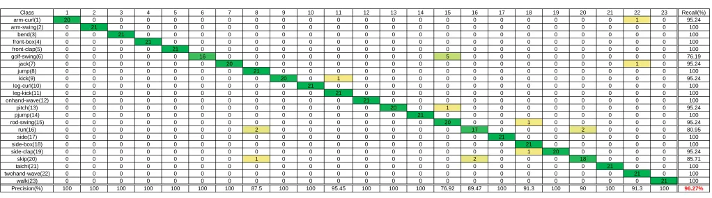
[image:11.612.51.562.220.362.2]Precision(%) 100 100 100 100 100 100 100 87.5 100 100 95.45 100 100 100 76.92 89.47 100 91.3 100 90 100 91.3 100 96.27%
Figure 16. Confusion matrix of our method with improved DMMs on theDHAdataset. The number in red indicates the overall accuracy.
Class 1 2 3 4 5 6 7 8 9 10 11 12 Recall(%)
z(1) 27 0 1 0 0 0 0 0 0 0 0 0 96.43
j(2) 0 27 0 0 0 0 0 0 0 1 0 0 96.43
where(3) 0 0 28 0 0 0 0 0 0 0 0 0 100
store(4) 0 0 0 28 0 0 0 0 0 0 0 0 100
pig(5) 0 0 0 0 25 0 0 0 0 0 0 0 100
past(6) 0 0 0 0 0 28 0 0 0 0 0 0 100
hungry(7) 0 0 0 0 0 0 28 0 0 0 0 0 100
green(8) 0 0 0 0 0 0 0 28 0 0 0 0 100
finish(9) 0 0 0 0 0 0 0 0 28 0 0 0 100
blue(10) 0 0 0 0 0 0 0 0 0 28 0 0 100
bathroom(11) 0 0 0 0 0 0 0 0 0 0 28 0 100
milk(12) 0 0 0 0 0 0 0 0 0 0 0 28 100
Precision(%) 100 100 96.55 100 100 100 100 100 100 96.55 100 100 99.39%
Figure 17. Confusion matrix of our method with improved DMMs on theMSRGesture3Ddataset. The number in red indicates the overall accuracy.
The best performance results are shown in Figure 15,16,17,18,19. In Figure 15, the confusion matrix of the
MSRAction3D dataset is shown with an accuracy of 96.70%. It is observed that large ambiguities exist between similar action pairs, for example “handCatch” and “highThrow”, and “drawX” and “drawTick”, due to the similarities of their DMMs. In Figure 16, the confusion matrix of our method on the DHA dataset is shown with an accuracy of 96.27%. In Figure 17, the confusion matrix of the MSRGesture3D
dataset is shown with an accuracy of 99.39%. It is observed that similar action pairs like “milk” and “hungry” can be distinguished with high accuracy. The confusion matrices of the MSRAction3D-Speed dataset is shown in Fig. 18, where the action “drawX” and “drawTick” have maximum confusion with each other since both actions contain similar motion
and appearance. The recall rate and precision for most of the actions are beyond 91.57%, which verifies the robustness of our method to speed variations. In Figure 19, the confusion matrix of the MSRDailyActivity3D dataset is shown with an accuracy of89.00%, indicating that our method can properly handle human-object interactions.
V. CONCLUSION
[image:11.612.53.563.388.527.2]Class 1 2 3 4 5 6 7 8 9 10 11 12 13 14 15 16 17 18 19 20 Recall(%)
highArmWave(1) 12 0 0 0 0 0 0 0 0 0 0 0 0 0 0 0 0 0 0 0 100
horizArmWave(2) 0 12 0 0 0 0 0 0 0 0 0 0 0 0 0 0 0 0 0 0 100
hammer(3) 0 0 9 0 1 1 0 1 0 0 0 0 0 0 0 0 0 0 0 0 75
handCatch(4) 0 0 0 7 1 1 0 1 0 0 0 0 0 0 2 0 0 0 0 0 58.33
forwardPunch(5) 0 0 0 0 9 0 0 0 0 0 0 0 0 0 0 0 2 0 0 0 81.82
highThrow(6) 0 0 0 1 0 10 0 0 0 0 0 0 0 0 0 0 0 0 0 0 90.91
drawX(7) 0 0 0 0 0 0 9 3 0 0 0 0 0 0 0 0 0 0 1 0 69.23
drawTick(8) 1 0 0 0 0 0 0 13 1 0 0 0 0 0 0 0 0 0 0 0 86.67
drawCircle(9) 0 0 0 0 0 0 1 2 12 0 0 0 0 0 0 0 0 0 0 0 80
handClap(10) 0 0 0 0 0 0 0 0 0 15 0 0 0 0 0 0 0 0 0 0 100
twoHandWave(11) 0 0 0 0 0 0 0 0 0 0 15 0 0 0 0 0 0 0 0 0 100
side-boxing(12) 0 0 0 0 0 0 0 0 0 0 0 15 0 0 0 0 0 0 0 0 100
bend(13) 0 0 0 0 0 0 0 0 0 0 0 0 15 0 0 0 0 0 0 0 100
forwardKick(14) 0 0 0 0 0 0 0 0 0 0 0 0 0 15 0 0 0 0 0 0 100
sideKick(15) 0 0 0 0 0 0 0 0 0 0 0 0 0 0 9 0 0 0 2 0 81.82
jogging(16) 0 0 0 0 0 0 0 0 0 0 0 0 0 0 0 15 0 0 0 0 100
tennisSwing(17) 0 0 0 0 0 0 0 0 0 0 0 0 0 0 0 0 15 0 0 0 100
tennisServe(18) 0 0 0 0 0 0 0 0 0 0 0 0 0 0 0 0 1 14 0 0 93.33
golfSwing(19) 0 0 0 0 0 0 0 0 0 0 0 0 0 0 0 0 0 0 15 0 100
pickup&throw(20) 0 0 0 0 0 0 0 0 0 0 0 0 0 0 0 0 0 0 0 14 100
[image:12.612.52.562.54.192.2]Precision(%) 92.31 100 100 87.5 81.82 83.33 90 65 92.31 100 100 100 100 100 81.82 100 83.33 100 83.33 100 91.57%
Figure 18. Confusion matrix of our method with improved DMMs on the random sampling-basedMSRAction3D-Speeddataset. The number in red indicates the overall accuracy.
Class 1 2 3 4 5 6 7 8 9 10 Recall(%) drink(1) 10 0 0 0 0 0 0 0 0 0 100
eat(2) 0 10 0 0 0 0 0 0 0 0 100 call cellphone(3) 4 1 5 0 0 0 0 0 0 0 50
use vacuum(4) 0 0 0 10 0 0 0 0 0 0 100 cheer up(5) 0 0 0 0 9 0 1 0 0 0 90 toss paper(6) 1 0 3 1 0 5 0 0 0 0 50 lay down(7) 0 0 0 0 0 0 10 0 0 0 100
walk(8) 0 0 0 0 0 0 0 10 0 0 100 stand up(9) 0 0 0 0 0 0 0 0 10 0 100 sit down(10) 0 0 0 0 0 0 0 0 0 10 100 Precision(%) 66.67 90.91 62.5 90.91 100 100 90.91 100 100 100 89.00%
Figure 19. Confusion matrix of our method with improved DMMs on theMSRDailyActivity3Ddataset. The number in red indicates the overall accuracy.
the patch-based LBP feature extraction approach is adopted to characterize the rich texture information (e.g., edges, contours, etc.) in the LBP coded DMMs. The Fisher kernel represen-tation is considered to aggregate local patch features into a compact and discriminative representation. The proposed method is extensively evaluated on five benchmark datasets. The experimental results show that our method outperforms the state-of-the-art methods in all datasets. Additional tests on our collected MSRAction3D-Speed dataset confirm that our method is able to handle depth sequences which contain dramatic frame rate differences. With the implementation of kernel-based extreme learning machine (ELM) classifier, our method can classify actions accurately in real-time.
ACKNOWLEDGMENTS
This work was supported in part by the Natural Science Foundation of China (NSFC 61672079, 61473086, U1613209, 6167021685).
REFERENCES
[1] N. Zhao, L. Zhang, B. Du, L. Zhang, D. Tao, and J. You, “Sparse tensor discriminative locality alignment for gait recognition,” in2016 International Joint Conference on Neural Networks (IJCNN), July 2016, pp. 4489–4495.
[2] C. Chen, N. Kehtarnavaz, and R. Jafari, “A medication adherence monitoring system for pill bottles based on a wearable inertial sensor,” inEMBC, 2014, pp. 4983–4986.
[3] L. Zhang, L. Zhang, D. Tao, and B. Du, “A sparse and discriminative tensor to vector projection for human gait feature representation,”Signal Processing, vol. 106, no. Supplement C, pp. 245 – 252, 2015. [4] C. Chen, K. Liu, R. Jafari, and N. Kehtarnavaz, “Home-based senior
fitness test measurement system using collaborative inertial and depth sensors,” inEMBC, 2014, pp. 4135–4138.
[5] V. Bloom, D. Makris, and V. Argyriou, “G3d: A gaming action dataset and real time action recognition evaluation framework,” in CVPRW, 2012, pp. 7–12.
[6] D. W. Tjondronegoro and Y. P. P. Chen, “Knowledge-discounted event detection in sports video,” IEEE Transactions on Systems Man & Cybernetics: Systems, vol. 40, no. 5, pp. 1009–1024, 2010.
[7] H. Wang and C. Schmid, “Action recognition with improved trajecto-ries,” inICCV, 2013, pp. 3551–3558.
[8] X. Yang and Y. Tian, “Super normal vector for activity recognition using depth sequences,” inCVPR, 2014, pp. 804–811.
[9] B. Ni, G. Wang, and P. Moulin, “Rgbd-hudaact: A color-depth video database for human daily activity recognition,” in ICCVW, 2011, pp. 1147–1153.
[10] J. Shotton, A. Fitzgibbon, M. Cook, T. Sharp, M. Finocchio, R. Moore, A. Kipman, and A. Blake, “Real-time human pose recognition in parts from single depth images,” inCVPR, 2011, pp. 1297–1304.
[11] W. Li, Z. Zhang, and Z. Liu, “Action recognition based on a bag of 3d points,” inCVPRW, 2010, pp. 9–14.
[12] L. Xia and J. K. Aggarwal, “Spatio-temporal depth cuboid similarity feature for activity recognition using depth camera,” inCVPR, 2013, pp. 2834–2841.
[13] X. Yang, C. Zhang, and Y. L. Tian, “Recognizing actions using depth motion maps-based histograms of oriented gradients,” ACM MM, pp. 1057–1060, 2012.
[14] C. Chen, K. Liu, and N. Kehtarnavaz, “Real-time human action recog-nition based on depth motion maps,” Journal of Real-Time Image Processing, pp. 1–9, 2013.
[15] C. Chen, R. Jafari, and N. Kehtarnavaz, “Action recognition from depth sequences using depth motion maps-based local binary patterns,” in
WACV, 2015, pp. 1092–1099.
[16] B. Zhang, Y. Yang, C. Chen, L. Yang, J. Han, and L. Shao, “Action recognition using 3d histograms of texture and a multi-class boosting classifier,”IEEE Transactions on Image Processing, vol. 26, no. 10, pp. 4648–4660, Oct 2017.
[17] O. Oreifej and Z. Liu, “Hon4d: Histogram of oriented 4d normals for activity recognition from depth sequences,” in CVPR, 2013, pp. 716– 723.
[18] R. Vemulapalli, F. Arrate, and R. Chellappa, “Human action recognition by representing 3d human skeletons as points in a lie group,” inCVPR, 2014, pp. 588–595.
[image:12.612.128.483.234.326.2]and rotation invariant texture classification with local binary patterns,”
TPMAI, vol. 24, no. 7, pp. 971–987, 2002.
[20] F. Perronnin, J. Sanchez, and T. Mensink, “Improving the fisher kernel for large-scale image classification,” inECCV, 2010, pp. 143–156. [21] G. B. Huang, Q. Y. Zhu, and C. K. Siew, “Extreme learning machine:
Theory and applications,”Neurocomputing, vol. 70, no. 1-3, pp. 489– 501, 2006.
[22] C. Chen, M. Liu, B. Zhang, J. Han, J. Jiang, and H. Liu, “3D action recognition using multi-temporal depth motion maps and fisher vector,” inIJCAI, 2016.
[23] Y. Du, W. Wang, and L. Wang, “Hierarchical recurrent neural network for skeleton based action recognition,” inCVPR, 2015.
[24] J. K. Aggarwal and X. Lu, “Human activity recognition from 3d data: A review,”PRL, vol. 48, no. 1, pp. 70–80, 2014.
[25] S. Tang, X. Wang, X. Lv, T. X. Han, J. Keller, Z. He, M. Skubic, and S. Lao,Histogram of Oriented Normal Vectors for Object Recognition with a Depth Sensor. Springer Berlin Heidelberg, 2013.
[26] H. Rahmani, A. Mahmood, Q. H. Du, and A. Mian,HOPC: Histogram of Oriented Principal Components of 3D Pointclouds for Action Recog-nition. Springer International Publishing, 2014.
[27] C. Lu, J. Jia, and C. K. Tang, “Range-sample depth feature for action recognition,” inCVPR, 2014, pp. 772–779.
[28] H. Rahmani, Q. H. Du, A. Mahmood, and A. Mian, “Discriminative human action classification using locality-constrained linear coding,”
PRL, 2015.
[29] C. Chen, B. Zhang, Z. Hou, J. Jiang, M. Liu, and Y. Yang, “Action recognition from depth sequences using weighted fusion of 2d and 3d auto-correlation of gradients features,”Multimedia Tools and Applica-tions, pp. 1–19, 2016.
[30] C. Jia and Y. Fu, “Low-rank tensor subspace learning for rgb-d action recognition,”IEEE Transactions on Image Processing, vol. 25, no. 10, pp. 4641–4652, Oct 2016.
[31] H. Rahmani and A. Mian, “3d action recognition from novel view-points,” inCVPR, 2016.
[32] M. Zanfir, M. Leordeanu, and C. Sminchisescu, “The moving pose: An efficient 3d kinematics descriptor for low-latency action recognition and detection,” inICCV, 2013, pp. 2752–2759.
[33] T. Kerola, N. Inoue, and K. Shinoda,Spectral Graph Skeletons for 3D Action Recognition. Springer International Publishing, 2014. [34] X. Cai, W. Zhou, and H. Li, “Attribute mining for scalable 3d human
action recognition,” inACM MM, 2015, pp. 1075–1078.
[35] B. Du, W. Xiong, J. Wu, L. Zhang, L. Zhang, and D. Tao, “Stacked convolutional denoising auto-encoders for feature representation,”IEEE Transactions on Cybernetics, vol. 47, no. 4, pp. 1017–1027, April 2017. [36] “Enhanced skeleton visualization for view invariant human action
recog-nition,”Pattern Recognition, vol. 68, pp. 346–362, 2017.
[37] J. Wang, Z. Liu, and Y. Wu, “Learning actionlet ensemble for 3D human action recognition,”TPAMI, vol. 36, no. 5, pp. 1290–1297, 2014. [38] E. Ohn-Bar and M. M. Trivedi, “Joint angles similiarities and hog2 for
action recognition,” inCVPRW, 2013, pp. 465–470.
[39] A. F. Bobick and J. W. Davis, “The recognition of human movement using temporal templates,”TPAMI, vol. 23, no. 3, pp. 257–267, 2001. [40] J. Wang, Z. Liu, J. Chorowski, Z. Chen, and Y. Wu, “Robust 3d action
recognition with random occupancy patterns,” inECCV, 2012, pp. 872– 885.
[41] C. Zhang and Y. Tian, “Histogram of 3D facets: A depth descriptor for human action and hand gesture recognition,”CVIU, vol. 139, 2015. [42] G. Evangelidis, G. Singh, and R. Horaud, “Skeletal quads:human action
recognition using joint quadruples,” inICPR, 2014, pp. 4513–4518. [43] Y. Kong, B. Satarboroujeni, and Y. Fu, “Hierarchical 3d kernel
descrip-tors for action recognition using depth sequences,” inFG, 2015, pp. 1–6.
[44] M. Liu and H. Liu, “Depth context: A new descriptor for human activity recognition by using sole depth sequences,”Neurocomputing, pp. 747– 758, 2015.
[45] Y.-C. Lin, M.-C. Hu, W.-H. Cheng, Y.-H. Hsieh, and H.-M. Chen, “Human action recognition and retrieval using sole depth information,” inACM MM, 2012, pp. 1053–1056.
[46] L. Gorelick, M. Blank, E. Shechtman, M. Irani, and R. Basri, “Actions as space-time shapes,”TPMAI, vol. 29, no. 12, pp. 2247–2253, 2007. [47] H. Liu, L. Tian, and M. Liu, “Sdm-bsm: A fusing depth scheme for
human action recognition,” inICIP, 2015, pp. 4674–4678.
[48] Z. Gao, H. Zhang, G. P. Xu, and Y. B. Xue, “Multi-perspective and multi-modality joint representation and recognition model for 3d action recognition,”Neurocomputing, vol. 151, pp. 554–564, 2015.
[49] H. Rahmani, A. Mahmood, D. Q. Huynh, and A. Mian, “Real time action recognition using histograms of depth gradients and random decision forests,” inWACV, 2014, pp. 626–633.
[50] J. Wang, Z. Liu, Y. Wu, and J. Yuan, “Mining actionlet ensemble for action recognition with depth cameras,” inCVPR, 2012, pp. 1290–1297. [51] A. Klaser, M. Marszalek, and C. Schmid, “A spatio-temporal descriptor
based on 3d-gradients,” inBMVC, 2008.