Autonomous Data Density based Clustering Method
Plamen P. Angelov
and Xiaowei Gu
School of Computing and Communications InfoLab21, Lancaster University,
Lancaster, LA1 4WA, UK. E-mail: [email protected]
German Gutierrez
and Jose Antonio Iglesias
and Araceli Sanchis
Computer Science Department
Carlos III University of Madrid, Madrid, Spain, E-mails:{ggutierr, jiglesia, masm}@inf.uc3m.es
Abstract—It is well known that clustering is an unsupervised machine learning technique. However, most of the clustering methods need setting several parameters such as number of clusters, shape of clusters, or other user- or problem-specific parameters and thresholds. In this paper, we propose a new clustering approach which is fully autonomous, in the sense that it does not require parameters to be pre-defined. This approach is based on data density automatically derived from their mutual distribution in the data space. It is called ADD clustering (Autonomous Data Density based clustering). It is entirely based on the experimentally observable data and is free from restrictive prior assumptions.
This new method exhibits highly accurate clustering perfor-mance. Its performance is compared on benchmarked data sets with other competitive alternative approaches. Experimental re-sults demonstrate that ADD clustering significantly outperforms other clustering methods yet does not require restrictive user- or problem-specific parameters or assumptions. The new clustering method is a solid basis for further applications in the field of data analytics.
Index terms- fully autonomous clustering; data density; mutual distribution; data analytics.
I. INTRODUCTION
Clustering has long been widely used for finding underlying groups and patterns within the data. We have already entered the Era of Big Data. Clustering as an unsupervised machine learning method is currently a very hot topic in the field of data processing and considered as one of the most effective tools for extracting information from data and, thus, one of the ways to address the Big Data problems.
Traditional clustering methods require user inputs based on some priorknowledge or different assumptions (including number of clusters, the shape of clusters, etc.) to work effi-ciently. In most practical cases, however, thepriorknowledge is very limited and the assumptions made are always too ideal to be true. The requirement ofpriorknowledge or assumptions does, no doubt, limit the traditional clustering methods abilities in data analytics and information discovery [1].
In this paper, we propose a new autonomous clustering algorithm named ADD clustering (Autonomous Data Density-based clustering). The novelty of this new algorithm is that it is entirely based on the data and their mutual distribution in the data space. There is no need for predefined spe-cific thresholds or any kind of user inputs in the proposed method. Additionally, ADD clustering method works equally
effectively with various types of distance/similarity metrics and arbitrary number of dimensions of data. It starts from scratch, self-defines the data pattern in terms of density, and exhibits a highly accurate clustering performance. To the best of our knowledge, this is the first clustering method with such characteristics of real autonomy.
The remainder of this paper is organized as follows: section II introduces some related published techniques for further comparison. Section III provides the theoretical ba-sis of the proposed method. The detailed demonstration of ADD clustering method is given in section IV. Experimental results and analysis are shown in section V and section VI is providing the conclusions.
II. RELATEDWORK
The clustering problems has been addressed in different context in many disciplines such as data mining, information retrieval or pattern recognition. However, as far as we know, there is still no clustering method which does not require any kind of user- or problem- specific parameter. Nonetheless, our proposed method will be compared with several well-known methods, such as mean shift clustering, K-means clustering, as well as with some recent advanced (DDCAR [2] and eClustering[3]) methods. These four methods need some kind of priorknowledge. In this section, we will detail their most important aspects.
• Mean shift clustering [4] method considers an empirical probability distribution function around the data samples and the cluster centres or modes of the underlying dis-tribution are represented by dense regions in the data space. After each iteration, the candidate solution shifts closer to the nearest mean and, finally, converges to the nearest mode or cluster centre. The direction of change is estimated by the gradient of the kernel density. The Mean shift clustering method requires the user to pre-define the kernel size. Clustering results are susceptible to different kernel sizes. Without anypriorknowledge of the data, it is very hard to decide the kernel sizes.
samples are reassigned again. This process continues until the clusters do not change any more. The K-means clustering method supports different types of distances as well as high dimensional data. Despite of its excellent performance, k-means clustering algorithm requires a user input, namely the number of clusters, which is an impossible task for users withoutprior knowledge. • DDCAR [2] method is also based on the data density.
By using the data density calculations to estimate the initial radius, DDCAR can be defined as a data-driven automated clustering method. Compared with other cur-rent clustering methods,DDCARonly needs users to set the minimum size of clusters, which is a great advance. However, DDCARis still not totally free of user input. The minimum size of clusters can still influence the accuracy of the method. In addition, DDCAR currently only supports 2-dimensional data with Euclidean type of distance.
• Evolving clustering (eClustering) uses proximity based potential value to determine the cluster centres. The favourite characteristics of eClustering [3] are that it automatically identifies the number of clusters and also handles the outliers. Nonetheless, eClustering requires users to decide the initial radius of the clusters. The initial radius of clusters will be different with various types of datasets. As a result, deciding the initial radius will need users to havepriorknowledge on the data, oreClustering might not achieve the best performance.
III. THEORETICALBASISOF THEPROPOSEDMETHOD
In this section, three cornerstone non-parametric estimators of data ensemble properties (cumulative proximity, density, eccentricity, typicality) defined within the TEDA framework [1], [6], [7] and used within the proposed ADD clustering method will be described.
First of all, let us define several basic notions. In this paper, Rp is defined as the real data space consisted of p dimensional data points.{x1, x2, . . . , xk} is a series of data points belonging to Rp,k denotes the time instant when the last data sample arrives.
Within the data spaceRp, the distanced(x, y)is defined as a measurement of dissimilarity between the two data pointsx
andy. The proposed ADD clustering algorithm can work with various types of distance metrics including Euclidean, Maha-lanobis, and a recently introduced, direction-aware distance [6] metric.
A. Cumulative Proximity
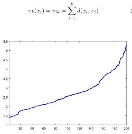
Cumulative proximity, πk is a representation of the close-ness of a certain data point to all other data points, which is obtained in a direct way by summing the distance or dissimilarity measures between all points, see Fig.1 as an example of the cumulative proximity for a dataset which has
100 data samples per cluster:
πk(xi) =πik= k
X
j=1
[image:2.612.330.554.57.283.2]d(xi, xj) (1)
Fig. 1: Example of cumulative proximity
For the case of Euclidean type of distance, we have [1], [6], [7]:
πk(xi) =k((x−µk)T(x−µk) +Xk−µTkµk) (2)
For Mahalanobis type of distance, we have [1], [6], [7]:
πk(xi) =k((x−µk)TΣk−1(x−µk) +Xk−µTkΣ −1
k µk) (3)
whereXk =1kPki=1xTi
P−1
k xi
Normally, the data points which are close to the centre of the group will have much lower cumulative proximity than the data points close to the edge of the group. Thus, naturally, outliers will have high πk value and a point with minimum
πk is a natural candidate to be a cluster centre.
B. Eccentricity
Eccentricity [1], [7] is another very important indicator of the ensemble properties of the data. It plays a critical role in the proposed method.
Eccentricity can be considered as normalized cumulative proximityπk and is defined as follows [6]:
ξk(x) =
2πk(x)
Pk
i=1πk(xi)
,
k
X
i=1
πk(xi)>0 k >1 (4)
where the normalization coefficient 2 is due to the fact that, in the sum, each distance is counted twice [1], [7]. Obviously, the range of eccentricity values is from 0 to 1 and it sums to 2 [1], [7].
problem, the standardized eccentricity is also introduced [6] as:
k(x) =kξk(x) =
2πk(x)
E(πk(x))
, E(πk(x))>0 k >1 (5)
where E(πk(x)) = 1k
Pk
i=1πk(x) is the mean cumulative proximity. Correspondingly, the range of possible values for
k(x)is1< k(x)< k
and the sum of all k(x)values is
k
X
i=1
k(xi) = 2k (6)
C. Data Density
Density plays a very important role in the proposed algo-rithm. Data density is inversely proportional to the eccentricity and is defined in [6] as:
Dk(xi) = 1
k(xi)
=E(πk(x)) 2πk(xi)
(7)
Obviously, the closer a particular data point is to other points, the smaller its cumulative proximity is, and the higher its density is. Although, cumulative proximity and density can both provide effective information about the data pattern, density is comparatively superior because it is: 1) Monotonic; 2) Maximum value is 1; 3) Asymptotically tends to zeros when
πk tends to infinity. Therefore, it has properties similar to a likelihood and probability [6].
IV. ADD CLUSTERINGALGORITHM
ADD clustering is a novel method based entirely on the empirical observations (discrete data samples) and the density of this data. The proposed method does not require any user-or problem- specific threshold to be predefined and can extract the cumulative proximity, eccentricity and density of the data samples. Compared with other previously published methods, the proposed ADD clustering algorithm has the following advantages:
• No priorknowledge of the dataset is needed; • No initial user input is required;
• Entirely based on the data and its mutual distribution in the data space;
• No need to choose a model of the data distribution (e.g. Gaussian, etc.).
In the remaining part of this section we will explain in detail the three stages of our method: 1) initial centre and radius formation; 2) centre and radius updating; 3) clusters final adjustment.
A. Stage 1. Initial Centre and Radius
The first stage of our method consists in finding out the initial centre and radius of the new cluster in the particular datasets {x1, x2, . . . , xk}. The global cumulative proximity
πk(x), eccentricity ξ (or standardised eccentricity k(x)), density Dk(x) of every data point are obtained by formulas
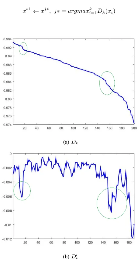
(1),(4),(5), and (7). By ranking the global density values of all data points in descending order, the data point with the highest density is selected as the initial centre of the newly formed cluster:
x∗1←xj∗, j∗=argmaxki=1Dk(xi) (8)
(a)Dk
[image:3.612.324.551.103.530.2](b)Dk0
Fig. 2: Examples of ranked global density(Dk) and smoothed differential density(D0k)
Because, the density is higher closer to the cluster centres and lower towards the edges, there would always be a change in the gradient of the density when data samples belonging to different clusters are grouped together. It is well known that the change of gradient is an indication of an inflexion point and change of the sign of the second derivative [8]. As we can see in the example in Fig.2a (based on the dataset as previously described), there are several inflexion points in the rate of density reduction, which indicate the end/edge of a cluster.
should be further processed by applying a moving window average difference operation to zoom in as follows:
D0k(x) = 1
N
N−1 X
i=0
[Dk(x+i+N)−Dk(x+i)] (9)
where 2N is the width of the moving window, a value of
N = 6 can be used for all problems and data sets. It has to be stressed that the value 6 is not a problem- or user- specific parameter and is the same for all problems. Moreover, its slight variations do not influence the result. It is merely a way to zoom in and focus on the changes of Dk.
Compared with regular difference operation [2] , the average difference operation is less susceptible to the influence of noise and different data patterns, namely it is more robust.
After the moving window average difference operation is applied, the smoothed differential density D0
k(x) will have larger drops/jumps as shown in Fig. 2b (based on the same data as previously).
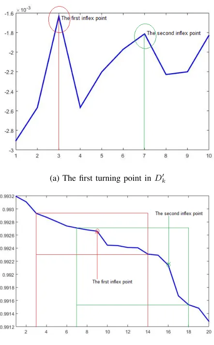
To ensure the purity [9] of the initial members of the new cluster, we select the first turning point of D0k(x), which indicates that there is a change in the speed of the descent of the densities in the data points shown in Fig. 3.
Then, the initial radius of the new cluster can be defined by calculating the distance between the initial centre and the first inflexion point point,Dk(x+ 2N−1). By finding all data points within the distance of the initial radius from the initial centre, the prototype of a new cluster is obtained, and the first step is finished.
B. Stage 2. Centre and Radius Updating
At the end of the previous stage, a prototype of the newly formed cluster is built, but the cluster is not fully formed yet; we should update the centre and radius to let in more samples belong to the new cluster.
Again, formulas (2), (4), (5) and (7) are used to calculate the local density and the equation (9) is used for smoothing and differencing the localdensity after it is ranked in descending order. We denote the smoothed differential local density as
D0L(x).
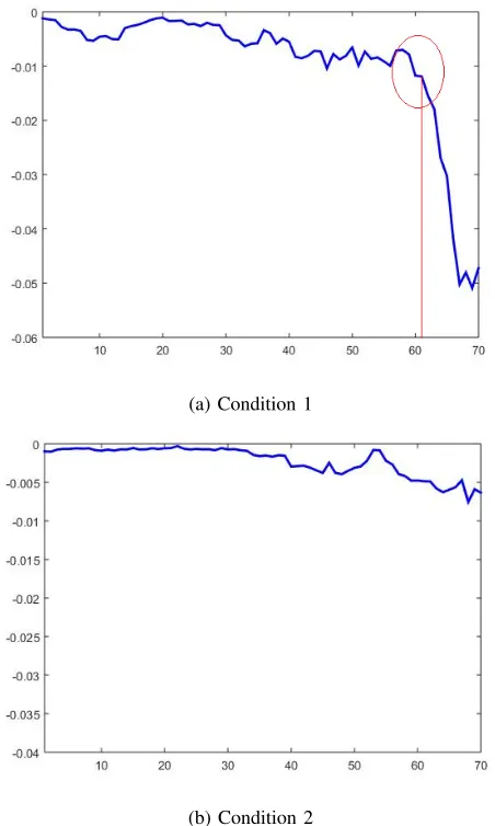
There are two conditions that can occur in regards to the smoothed differential localdensity.
Condition 1. There is a big drop in DL0(x);
Condition 2. There is only a steady drop with normal fluctuations inD0L(x).
Examples of Conditions 1 and 2 are shown in Fig. 4a and 4b respectively using the same data as the previous.
The well-known Chebyshev inequality [10] describes the probability that certain data samplexis more thannσdistance away from the mean value. For Euclidean type of distance it has the following form:
P(kµ−xk2≤n2σ2)≥1− 1
n2 (10)
Here, we use the Chebyshev inequality to help us distinguish the two conditions:
(a) The first turning point inD0k
[image:4.612.329.550.50.406.2](b) The corresponding changing area inDk
Fig. 3: Examples of the first turning point in the smoothed differential density(D0k) and the ranked global density(Dk)
Condition 1:(D0L(xm)−µL)2≥n2σ2L (11)
Condition 2:(D0L(xm)−µL)2< n2σ2L (12)
wherexm is the data point having the maximum value in
DL0(xm)in the new cluster, theµL andσL are the mean and standard deviation ofD0L(x1), D0L(x2). . . DL0(xm−1).n= 3
is used for all problems and is well known from the literature [10].
If condition 1 is met, it means that the new cluster actually contains samples from two or more clusters. The transition between the two clusters is exactly the point when DL0(x) drops. The centre of the new cluster is updated based on the points that belong to this cluster, and the radius of the newly formed cluster is updated by:
r=kx1−xmk (13)
(a) Condition 1
[image:5.612.63.289.59.436.2](b) Condition 2
Fig. 4: Illustrative examples of the smoothed differentiallocal density
enlarged letting all samples of this initial cluster to be included in the new cluster.
After the centre and radius become stable during updating and the members of the newly formed cluster do not change any more, we can declare that the centre and radius updating operation is finished and a new cluster is formally formed. Then, we can remove all the data points belonging to the new cluster from the dataset and go back to stage 1 to form another cluster.
C. Stage 3. Clusters Final Adjustment
When all the possible clusters have already been formed and the data points left in the dataset are not available to form a new cluster, stages 1 and 2 are finished, but the clusters formed are not always ideal. Because of the fact that the clusters are formed one by one sequentially, and in each time only one new cluster is formed, sometimes there will be overlaps between the spreads of influences of some clusters. Therefore,
the clusters should be adjusted before the whole clustering process is finished.
First of all, we define several conditions:
Condition 3. If the distance between the centres of two clusters satisfies the following inequality:
x∗i −x∗j
≤min(ri, rj) (14)
Then the two clusters are defined as double-centres-overlapped.
Here x∗
i and x∗i denote the centres of the i-th and j-th clusters, ri andrj are the radii correspondingly.
Condition 4. If the distance between the centres of two clusters satisfies the following inequality:
min(ri, rj)<
x∗i −x∗j
≤max(ri, rj) (15)
Then the two clusters are defined as single-centre-overlapped.
Condition 5. If the distance between the centres of two clusters satisfies the following inequality:
max(ri, rj)<
x∗i −x∗j
≤ri+rj (16)
Then the two clusters are defined asslightly-overlapped. Condition 6. If more than half of the members of a cluster are closer to the centres of its neighbouring clusters than to their own centre, namely for them
x
k i −x∗j
<
x
k i −x∗i
(17)
Then the cluster is defined as a loose cluster. Here xk i is thek-th member of thei-thcluster.
Condition 7. If more than half of the members of a cluster are in the area of influences of two or more clusters, namely:
x
k i −x∗j
< rj (18)
Then we regard this cluster as being group-covered by others.
Condition 8. If the average distance of the members of a cluster to the centre of a nearby cluster is smaller than its radius, namely:
1
Mi Mi X
k=1 xki −x∗j
< rj (19)
Then we regard this cluster as beingsingle-coveredby some other cluster(s). Here M is the member number of the i-th cluster.
If there are loose clusters, clusters being double-centres-overlapped, clusters being single-centre-overlapped by more than two clusters or clusters beinggroup-covered, we call these significantly overlapping cases.
If there are clusters being slightly-overlapped or clusters being single-centre-overlapped by one cluster, we call these slightly overlapping cases.
The final adjustment is divided into three steps.
Step 1: in this step, we will eliminate all the significantly overlapping cases.
Firstly, we check Rule 1.
Rule 1: If cluster Ci meets condition 6, and is double-centres-overlapped or single-centre-overlapped with most other clusters, thenCi should be split and all its members are re-assigned to the nearest clusters according to the following formula:
Cluster label=argmini=1,2,...,Kkx−x∗ik (20)
whereK is the number of clusters. Then, Rule 2 and Rule 3 are executed:
Rule 2: If clustersCi, Cj, . . .meet Condition 3 in regard to them, then clusters Ci, Cj, . . . should merge together.
Rule 3: If cluster Ci meets condition 3 with Cj, Ck, . . . whileCj, Ck, . . .only meets condition 4, then the largest one in Ci, Cj, Ck, . . .should be split and all its members are re-assigned to the nearest clusters using equation (20).
Because of the execution of the three rules above, the original structure of existing clusters is being changed largely, most of the significantly overlappingclusters have been split or merged, Rule 4 is used further to clear the remaining cases. Rule 4: If clusterCi meets Condition 6 or Condition 7, or is single-centre-overlapped by more than three clusters, then clusterCi should be split and all its members are re-assigned to the nearest clusters using equation (20).
Once Rules 1-4 are not used any more, Step 1 is finished and the final adjustment comes to Step 2.
Step 2: Since thesignificantly overlapping caseshave been resolved, the moderately overlapping cases are eliminated in this step, here, Rule 5 and Rule 6 are used.
Rule 5: If cluster Ci is single-centre-overlapped by two clusters then cluster Ci should be split and all its members are re-assigned to the nearest clusters using equation (20).
Rule 6: If clusterCiissingle-centre-overlappedand single-covered by cluster Cj, then Ci and Cj should be merged together.
Once there is one cluster that meets Rules 5 and 6 any more, all themoderately overlapping cases have been removed and the final adjustment comes to the last step.
Step 3: In this step, we simply find all the slightly over-lapping cases and reassign the members of the overlapping clusters, which meet equation (18), to the nearest clusters using equation (20).
Finally, for the remaining data points, we assign them to the nearest clusters using equation (20), which concludes the final adjustment.
D. Overall Clustering Process
The overall clustering process is summarised as follows Algorithm ADD clustering:
• A. Whileremaining data points in the dataset are available (or able to form a new cluster):
1) Calculate the global density,Dk of each data point by equation (7);
2) Rank the global density,Dkin descending order and smooth the ranked densities by equation (8); 3) Detect the first inflexion point, see Fig.3a;
4) Declare the initial centre x∗i and radiusri and find the initial cluster members;
5) While the members of the new cluster are still changing their allocation
– Calculate the local density,DL, of the new clus-ter;
– Rank the local density in descending order and smooth the ranked densities;
– If(Condition 1 or Condition 2 is met) Then: ∗ Update the radius and all data points that
belong to the new cluster; – End If
6) End While
7) A new cluster is formed;
8) Remove from the dataset the data points that belong to the new cluster;
• End While
• B. Whilethe existing clusters exhibit overlaps 1) Whilethere are significantly overlapping cases
– If(Rule 1 is met)Then
∗ Split the cluster and reassign the members to the nearest cluster by equation (20);
– End If
– If(Rule 2 is met)Then ∗ Merge the clusters; – End If
– If(Rule 3 is met)Then
∗ Split the cluster and reassign the members to the nearest cluster by equation (20);
– End If
– If(Rule 4 is met)Then
∗ Split the cluster and reassign the members to the nearest cluster by equation (20);
– End If 2) End While
3) Whilethere is nosignificantly overlapping caseany more
– If(Rule 5 is met)Then
∗ Split the cluster and reassign the members to the nearest cluster by equation (20);
– End If
– If(Rule 6 is met)Then ∗ Merge the clusters; – End If
5) While there is nosignificantly overlapping case or moderately overlapping caseany more
– If (slightly overlapping caseis found)Then ∗ Reassign the overlapping members to the
near-est clusters by equation (20); – End If
6) End While
• C.Assign remaining unclustered data points to the nearest clusters by equation (20);
• End ADD clustering
V. EXPERIMENTAL RESULTS AND ANALYSIS
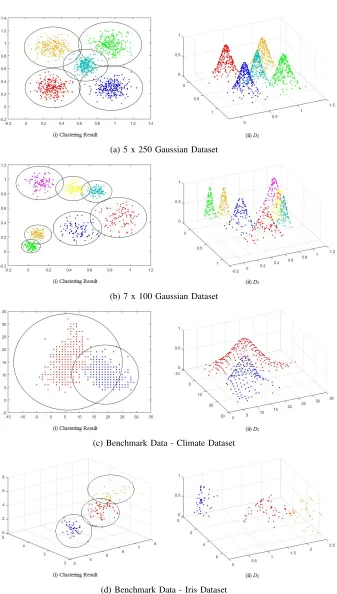
In order to test the performance of the newly proposed ADD clustering method, several artificial and benchmark datasets were used in numerical experiments. The artificial datasets were used to test the accuracy of the method, and the benchmark datasets were used to ensure that the method is applicable to real cases.
A. Datasets
Two artificial and two benchmark datasets were used in experiments with Euclidean type of distance:
1) The first dataset contained 5 clusters with 250 samples per cluster.
2) The second dataset had 7 clusters with 100 samples in each one.
3) Climate Dataset [11]. 4) Iris Dataset [12].
The datasets include clusters with very close proximity and chains of noise. The clustering results and the data density values are shown in Fig. 5.
B. Results
For further comparing, the quality of the proposed ADD clustering method with different existing methods in-cluding Mean-shift clustering, K-means clustering, DDCAR and eClustering, a number of measures of the performance were considered:
1) Input: the parameters that have to be predefined. 2) NoC: is the number of clusters in the result.
3) Accuracy: is a measure of the number of samples that are correctly assigned to their original clusters.
4) AverPurity: is a measure of the average purity of the clusters but can disguise poor results [9].
5) MaxPurity: is the maximum cluster purity [9]. 6) MinPurity: is the minimum cluster purity [9].
In this paper, the quality of clustering and the number of clusters in the results together directly decide the correctness and effectiveness of the proposed ADD clustering method. In order to get the most accurate result, the number of clusters should be exactly the same with the original dataset, and the clustering accuracy should be as high as possible. Therefore, clustering accuracy and NoC both are the most important measures. In this paper, the focus is on a new method for data
analytics, which is based entirely on the empirical observations of data samples and the cumulative proximity of these data.
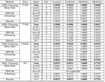
The comparative results for the artificial and benchmark datasets with Euclidean type of distance are shown in Table I, whereks denotes the kernel size in the mean shift clustering method; mcs denotes the minimum cluster size in DDCAR method;rdenotes the initial radius in eClusteringmethod;N denotes the number of clusters in theK-meansalgorithm.
Analysing the results, we can compare ADD clustering method with the other techniques listed above as follows:
• Mean shiftclustering method: Although, there are no re-quirement regarding thepriorinformation of the number of clusters and the embedded assumptions on the shape of the clusters, Mean shift clustering method actually needs users to predefine the kernel size. As we can see from the table, different kernel sizes can largely influence the clustering result. To exhibit good clustering performance using the mean shift clustering method, users have to decide the kernel size first either based on priorknowledge or trying many times before finding the ultimate one.
• K-meansclustering method has quite high accuracy com-pared with other algorithms, and can additionally work with different types of distance metrics. However, the high accuracy is based on the prior knowledge of the number of clusters in the datasets, which normally is unknown for users. With enough prior-knowledge, K-means clustering is quite accurate.
• DDCAR algorithm is comparable with ADD Clustering in terms of user input, but needs users to predefine the minimum size of clusters, which requires some prior knowledge about the datasets compared with other tech-niques. However, ADD Clustering is totally free of any user input. The results of DDCAR algorithm normally contain many clusters with few members. The distribution of the datasets can be misrepresented largely. In contrast, ADD Clustering can give clustering results with fewer and much more accurate clusters, which effectively reflect the distribution of datasets. In addition, DDCAR is not applicable for clustering the datasets with more than 2 di-mensions, which is also a serious disadvantage compared with ADD Clustering.
• eClusteringalgorithm requires users to select the original radius of clusters. As we can see in the Table 1, the selection of the initial radius can influence the clustering results largely. Choosing the most suitable initial radius can be a very hard task for users without any prior knowledge of the datasets. In addition, accuracy and purity is not as high as all other methods.
(a) 5 x 250 Gaussian Dataset
(b) 7 x 100 Gaussian Dataset
(c) Benchmark Data - Climate Dataset
[image:8.612.142.479.42.636.2](d) Benchmark Data - Iris Dataset
Fig. 5: The four datasets (two artificial, Climate and Iris) used in the experimentation.
VI. CONCLUSION
A novel, fully autonomous clustering method, ADD clustering, is introduced in this paper. The proposed
TABLE I: Clustering Results Comparison with Euclidean Type of Distance
Methods Data Inputs NoC Accuracy AverPurity MaxPurity MinPurity
ADD Clustering 5*250 None 5 0.9928 0.9928 1.0000 0.9690
Mean Shift ks=0.1 9 0.9640 0.9864 1.0000 0.9394
ks=0.2 5 0.9928 0.9928 1.0000 0.9690
DDCAR mcs=10 24 0.9125 0.9152 1.0000 0.5000
eClustering r=0.05 2 0.2712 0.2712 0.6692 0.2238
r=0.01 2 0.2712 0.2712 0.6692 0.2238
Kmeans N=5 5 0.9928 0.9928 1.0000 0.9840
ADD Clustering 7*100 None 7 0.9986 0.9986 1.0000 0.9615
Mean Shift ks=0.1 11 0.9029 0.9914 1.0000 0.9709
ks=0.2 5 0.7114 0.7114 1.0000 0.4975
DDCAR mcs=10 17 0.9571 0.9786 1.0000 0.9259
eClustering r=0.05 5 0.4771 0.5129 1.0000 0.3636
r=0.01 1 0.4771 0.5300 1.0000 0.3636
Kmeans N=7 7 0.7929 0.8529 1.0000 0.5025
ADD Clustering Climate None 2 0.9824 0.9824 0.9883 0.9764
Mean Shift ks=4 7 0.7141 0.9741 1.0000 0.9474
ks=6 2 0.9474 0.9474 0.9976 0.9773
DDCAR mcs=10 7 0.5141 0.5224 1.0000 0.5149
eClustering r=0.5 1 0.5071 0.5071 0.5071 0.5071
r=0.01 1 0.5071 0.5071 0.5071 0.5071
Kmeans N=2 2 0.9824 0.9824 0.9883 0.9764
ADD Clustering Iris None 3 0.8933 0.8933 1.0000 0.7742
Mean Shift ks=0.8 5 0.6867 0.8133 1.0000 0.5455
ks=1.2 2 0.6667 0.6667 1.0000 0.5000
DDCAR mcs=10 Not applicable
eClustering r=0.5 4 0.6067 0.6733 1.0000 0.5797
r=0.01 4 0.5533 0.6733 1.0000 0.5246
Kmeans N=3 3 0.8933 0.8933 1.0000 0.7742
Numerical experiments show that, without any user input, this method can exhibit excellent clustering performance compared with other methods that use various kinds ofprior knowledge or assumptions. Because of the advantages of no requirement for user inputs and self-generating the estimators of ensemble data properties of the clustered datasets, this new method is a very attractive and effective tool in the field of data analytics.
ACKNOWLEDGMENT
The first author would like to acknowledge the partial sup-port through The Royal Society grant IE141329/2014 Novel Machine Learning Paradigms to address Big Data Streams and the Chair of Excellence Programme of the Carlos III University of Madrid for the support of this work. This work has been partially supported by the Spanish Government under project TRA2013-48314-C3-1-R.
REFERENCES
[1] A. Plamen, “Outside the box: an alternative data analytics framework,”
Journal of Automation, Mobile Robotics and Intelligent Systems, vol. 8, no. 2, pp. 29–35, 2014.
[2] R. Hyde and P. Angelov, “A fully autonomous data density based clustering technique,” inEvolving and Autonomous Learning Systems (EALS), 2014 IEEE Symposium on, 2014, pp. 116–123.
[3] P. Angelov and D. Filev, “An approach to online identification of takagi-sugeno fuzzy models,”Systems, Man, and Cybernetics, Part B: Cybernetics, IEEE Transactions on, vol. 34, no. 1, pp. 484–498, Feb 2004.
[4] K. Fukunaga and L. Hostetler, “The estimation of the gradient of a density function, with applications in pattern recognition,”Information Theory, IEEE Transactions on, vol. 21, no. 1, pp. 32–40, 1975.
[5] J. MacQueen, “Some methods for classification and analysis of multi-variate observations,” inProceedings of the Fifth Berkeley Symposium on Mathematical Statistics and Probability, Volume 1: Statistics. Berkeley, Calif.: University of California Press, 1967, pp. 281–297.
[6] P. Angelov, J. Principe, D. Kangin, and X. Gu, “A generalized methodol-ogy for data analysis,”Submitted to Information Sciences, vol. 0, no. 00, pp. 000–000, 0000.
[7] P. Angelov, “Anomaly detection based on eccentricity analysis.” in
EALS. IEEE, 2014, pp. 1–8.
[8] B. Galpin and A. Graham,Calculator Statistics. AB Books, 2002. [9] R. Baruah and P. Angelov, “Evolving local means method for clustering
of streaming data,” inFuzzy Systems (FUZZ-IEEE), 2012 IEEE Inter-national Conference on, June 2012, pp. 1–8.
[10] T. C. M. John G. Saw, Mark C. K. Yang, “Chebyshev inequality with estimated mean and variance,”The American Statistician, vol. 38, no. 2, pp. 130–132, 1984.