warwick.ac.uk/lib-publications
Original citation:
Schillings, Claudia and Stuart, A. M.. (2017) Analysis of the ensemble Kalman filter for inverse
problems. SIAM Journal on Numerical Analysis, 55 (3). pp. 1264-1290.
Permanent WRAP URL:
http://wrap.warwick.ac.uk/96051
Copyright and reuse:
The Warwick Research Archive Portal (WRAP) makes this work by researchers of the
University of Warwick available open access under the following conditions. Copyright ©
and all moral rights to the version of the paper presented here belong to the individual
author(s) and/or other copyright owners. To the extent reasonable and practicable the
material made available in WRAP has been checked for eligibility before being made
available.
Copies of full items can be used for personal research or study, educational, or not-for-profit
purposes without prior permission or charge. Provided that the authors, title and full
bibliographic details are credited, a hyperlink and/or URL is given for the original metadata
page and the content is not changed in any way.
Publisher’s statement:
© 2017
SIAM Journal on Numerical Analysis
http://dx.doi.org/10.1137/16M105959X
A note on versions:
The version presented here may differ from the published version or, version of record, if
you wish to cite this item you are advised to consult the publisher’s version. Please see the
‘permanent WRAP URL’ above for details on accessing the published version and note that
access may require a subscription.
PROBLEMS
CLAUDIA SCHILLINGS∗ AND ANDREW M. STUART†
Abstract. The ensemble Kalman filter (EnKF) is a widely used methodology for state estimation
in partial, noisily observed dynamical systems, and for parameter estimation in inverse problems. Despite its widespread use in the geophysical sciences, and its gradual adoption in many other areas of application, analysis of the method is in its infancy. Furthermore, much of the existing analysis deals with the large ensemble limit, far from the regime in which the method is typically used. The goal of this paper is to analyze the method when applied to inverse problems with fixed ensemble size. A continuous-time limit is derived and the long-time behavior of the resulting dynamical system is studied. Most of the rigorous analysis is confined to the linear forward problem, where we demonstrate that the continuous time limit of the EnKF corresponds to a set of gradient flows for the data misfit in each ensemble member, coupled through a common pre-conditioner which is the empirical covariance matrix of the ensemble. Numerical results demonstrate that the conclusions of the analysis extend beyond the linear inverse problem setting. Numerical experiments are also given which demonstrate the benefits of various extensions of the basic methodology.
Key words. Bayesian Inverse Problems, Ensemble Kalman Filter, Optimization
AMS subject classifications. 65N21, 62F15, 65N75
1. Introduction. The Ensemble Kalman filter (EnKF) has had enormous im-pact on the applied sciences since its introduction in the 1990s by Evensen and
cowork-ers; see [11] for an overview. It is used for both data assimilation problems, where
the objective is to estimate a partially observed time-evolving system sequentially in
time [17], and inverse problems, where the objective is to estimate a (typically
dis-tributed) parameter appearing in a differential equation [25]. Much of the analysis of
the method has focussed on the large ensemble limit [24,23,13,20,10,22]. However
the primary reason for the adoption of the method by practitioners is its robustness
and perceived effectiveness when used with small ensemble sizes, as discussed in [2,3]
for example. It is therefore important to study the properties of the EnKF for fixed ensemble size, in order to better understand current practice, and to suggest future directions for development of the method. Such fixed ensemble size analyses are
start-ing to appear in the literature for both data assimilation problems [19,28] and inverse
problems [15,14,16]. In this paper we analyze the EnKF for inverse problems, adding
greater depth to our understanding of the basic method, as formulated in [15], as well
as variants on the basic method which employ techniques such as variance inflation
and localization (see [21] and the references therein), together with new ideas
(intro-duced here) which borrow from the use of sequential Monte Carlo (SMC) method for
inverse problems introduced in [18].
LetG:X → Y be a continuous mapping between separable Hilbert spacesX and
Y. We are interested in the inverse problem of recovering unknownufrom observation
y where
y=G(u) +η.
Hereηis an observational noise. We are typically interested in the case where the
in-∗Mathematics Institute, University of Warwick, Coventry CV4 7AL, UK ([email protected]).
†Mathematics Institute, University of Warwick, Coventry CV4 7AL, UK ([email protected]).
1
version is ill-posed onY, i.e. one of the following three conditions is violated: existence of solutions, uniqueness, stability. In the linear setting, we can think for example of a compact operator violating the stability condition. Indeed throughout we assume
in all our rigorous results, without comment, thatY=RK forK∈Nexcept in a few
particular places where we explicitly state thatY is infinite dimensional. A key role
in such inverse problems is played by the least squares functional
Φ(u;y) =1
2kΓ
−1
2(y− G(u))k2
Y.
Here Γ>0 normalizes the model-data misfit and often knowledge of the covariance
structure of typical noiseηis used to define Γ.
When the inverse problem is ill-posed, infimization of Φ in X is not a
well-behaved problem and some form of regularization is required. Classical methods
include Tikhonov regularization, infimization over a compact ball inX and truncated
iterative methods [9]. An alternative approach is Bayesian regularization. In Bayesian
regularization (u, y) is viewed as a jointly varying random variable in X × Y and,
as-suming thatη∼N(0,Γ) is independent ofu∼µ0, the solution to the inverse problem
is theX −valued random variableu|y distributed according to measure
(1) µ(du) = 1
Zexp −Φ(u;y)
µ0(du),
whereZ is chosen so thatµis a probability measure:
Z:=
Z
X
exp −Φ(u;y)
µ0(du).
See [7] for details concerning the Bayesian methodology.
The EnKF is derived within the Bayesian framework and, through its ensemble properties, is viewed as approximating the posterior distribution on the random
vari-able u|y. However, except in the large sample limit for linear problems [23, 13, 20]
there is little to substantiate this viewpoint; indeed the paper [10] demonstrates this
quite clearly by showing that for nonlinear problems the large ensemble limit does
not approximate the posterior distribution. In [22], a related result is proved for the
EnKF in the context of data assimilaion; in the large ensemble size limit the EnKF is proved to converge to the mean-field EnKF, which provides the optimal linear estima-tor of the conditional mean, but does not reproduce the filtering distribution, except in the linear Gaussian case. A different perspective on the EnKF is that it consti-tutes a derivative-free optimization technique, with the ensemble used as a proxy for
derivative information. This optimization viewpoint was adopted in [15,14] and is the
one we take in this paper: through analysis and numerical experiments we study the properties of the EnKF as a regularization technique for minimization of the least-squares misfit functional Φ at fixed ensemble size. We do, however, use the Bayesian perspective to derive the algorithm, and to suggest variants of it.
In section 2 we describe the EnKF in its basic form, deriving the algorithm by
means of ideas from SMC applied to the Bayesian inverse problem, together with
in-vocation of a Gaussian approximation. Section 3describes continuous time limits of
the method, leading to differential equations, and in section4we study properties of
the differential equations derived in the linear case and, in particular, their long-time behavior. Using this analysis we obtain clear understanding of the sense in which the
the continuous time limit of the EnKF corresponds to a set of preconditioned gradient flows for the data misfit in each ensemble member. The common preconditioner is the empirical covariance matrix of the ensemble which thereby couples the ensemble members together and renders the algorithm nonlinear, even for linear inverse
prob-lems. Section5 is devoted to numerical studies which illustrate the foregoing theory
for linear problems, and which also demonstrate that similar ideas apply to nonlinear
problems. In section6 we discuss variants of the basic EnKF method, in particular
the addition of variance inflation, localization or the use of random search methods based on SMC, within the ensemble method; all of these methods break the invariant
subspace property of the basic EnKF proved in [15] and we explore numerically the
benefits of doing so.
2. The EnKF for Inverse Problems. Here we describe how to derive the iterative EnKF as an approximation of the SMC method for inverse problems. Recall
the posterior distributionµ given by (1) and define the probability measuresµn by,
forh=N−1,
µn(du)∝exp −nhΦ(u;y)µ0(du).
The measuresµnare intermediate measures defined via likelihoods scaled by the step
sizeh=N−1. It follows thatµN =µthe desired measure onu|y.Then
(2) µn+1(du) =
1
Zn
exp −hΦ(u;y)µn(du),
for
Zn =
Z
exp(−hΦ(u;y))µn(du).
Denoting byLnthe nonlinear operator corresponding to application of Bayes’ theorem
to map fromµn toµn+1we have
(3) µn+1=Lnµn .
We have introduced an articial discrete time dynamical system which maps the prior
µ0 into the posteriorµN =µ.A heuristic worthy of note is that although we look at
the datay at each ofN steps, the effective variance is amplified byN = 1/hat each
step, compensating for the redundant, repeated use of the data. The idea of SMC is
to approximate µn by a weighted sum of Dirac masses: given a set of particles and
weights{u(nj), w
(j)
n }Jj=1 the approximation takes the form
µn'
J
X
j=1
w(nj)δu n(j),
with δun(j) denoting the delta-Dirac mass located at un(j). The method is defined
by the mapping of the particles and weights at time n to those at timen+ 1. The
method is introduced for Bayesian inverse problems in [18] where it is used to study
the problem of inferring the initial condition of the Navier-Stokes equations from data.
In [4] the method is applied to the inverse problem of determining the coefficient of a
divergence form elliptic PDE from linear functionals of the solution; furthermore the
method is also proved to converge in the large particle limitJ → ∞.
In practice the SMC method can perform poorly. This happens when the weights
are negligible. The EnKF aims to counteract this by always seeking an approximation in the form
µn'
1 J
J
X
j=1
δu(jn)
and thus
µn+1'
1 J
J
X
j=1
δu(j)
n+1.
The method is defined by the mapping of the particles at time ninto those at time
n+ 1. Letun ={u
(j)
n }Jj=1. Then using equation (25) in [15] with Γ7→h−1Γ shows
that this mapping of particles has the form
(4) u(nj+1) =u(nj)+Cup(un)(Cpp(un) +h−1Γ)−1 y
(j)
n+1− G(u
(j)
n )
, j= 1,· · ·, J,
where
y(nj+1) =y+ξ(nj+1)
and, foru={u(j)}J
j=1, we define the operatorsCpp andCup by
Cpp(u) = 1
J J
X
j=1
G(u(j))− G
⊗ G(u(j))− G
,
Cup(u) = 1
J J
X
j=1
u(j)−u⊗ G(u(j))− G
, (5)
u= 1
J J
X
j=1
u(j), G= 1
J J
X
j=1
G(u(j)).
We will consider both the cases where ξ(nj+1) ≡ 0 and where, with respect to bothj
andn, theξ(nj+1) are i.i.d. random variables distributed according toN(0, h−1Γ). We
can unify by considering the i.i.d. family of random variablesξn(j+1) ∼N(0, h−1Σ) and
focussing exclusively on the cases where Σ = Γ and where Σ = 0. The theoretical
results will be solely derived for the setting Σ = 0, i.e. no artificial noise will be added to the observational data.
The derivation of the EnKF as presented here relies on a Gaussian
approxima-tion, which can be interpreted as a linearization of the nonlinear operatorLn in the
following way: in the large ensemble size limit, the EnKF estimate corresponds to
the best linear estimator of the conditional mean. See [12] for a general discussion of
Bayes linear methods and [22] for details in the context of data assimilation. Thus,
besides the approximation of the measures µn by aJ particle Dirac measure, there
is an additional uncontrolled error resulting from the Gaussian approximation, and
analyzed in [10]. In [27], the EnKF in combination with an annealing process is used
to account for nonlinearities in the forward problem by weight-correcting the EnKF. For data assimilation problems, similar techniques can be applied to improve the
per-formance of the EnKF in the nonlinear regime, see e.g. [5] and the references therein
In summary, except in the Gaussian case of linear problems, there is no
conver-gence to µn as J → ∞. Our focus, then, is on understanding the properties of the
algorithm for fixedJ, as an optimization method; we do not study the approximation
of the measureµ. In this context we also recall here the invariant subspace property
of the EnKF method, as established in [15]:
Lemma 1. If S is the linear span of {u(0j)}J
j=1 then u
(j)
n ∈ S for all (n, j) ∈ Z+× {1, . . . , J}.
3. Continuous Time Limit. Here we study a continuous time limit of the EnKF methodology as applied to inverse problems; this limit arises by taking the
parameter h, appearing in the incremental formulation (2) of the Bayesian inverse
problem (1), to zero. We proceed purely formally, with no proofs of the limiting
process, as our main aim in this paper is to study the behavior of the continuous time limits, not to justify taking that limit. However we note that the invariant
subspace property of Lemma1 means that the desired limit theorems are essentially
finite dimensional and standard methods from numerical analysis may be used to establish the limits. In the next section all the theoretical results are derived under
the assumption that G is linear and Σ = 0. However in this section we derive the
continuous time limit in a general setting, before specifying to the linear noise-free case.
3.1. The Nonlinear Problem. Recall the definition of the operatorCupgiven
by (5). We recall thatun ={u
(j)
n }Jj=1, and assume thatun≈u(nh) in (4) in the limit
h→0.The update step of the EnKF (4) can be written in the form of a time-stepping
scheme:
u(nj+1) =u(nj)+hC up
(un)(hCpp(un) + Γ)−1 y− G(u(nj))
+hCup(un)(hCpp(un) + Γ)−1ξ
(j)
n+1
=u(nj)+hCup(un)(hCpp(un) + Γ)−1 y− G(u(nj))
+h12Cup(un)(hCpp(un) + Γ)−1
√ Σζn(j+1) ,
where ζn(j+1) ∼ N(0, I) i.i.d.. If we take the limith→0 then this is clearly a tamed
Euler-Maruyama type discretization of the set of coupled Itˆo SDEs
du(j)
dt =C
up(u)Γ−1(y− G(u(j))) +Cup(u)Γ−1√ΣdW (j)
dt .
(6)
Using the definition of the operatorCup we see that
du(j)
dt =
1 J
J
X
k=1
G(u(k))− G, y− G(u(j)) +√ΣdW
(j)
dt
Γ u
(k)−u
, (7)
where
u= 1
J J
X
j=1
u(j), G= 1
J J
X
j=1
G(u(j))
and h·,·iΓ = hΓ−
1
2·,Γ−12·i with h·,·i the inner-product on Y. The W(j) are
inde-pendent cylindrical Brownian motions on X. The construction demonstrates that,
provided a solution to (7) exists, it will satisfy a generalization of the subspace
prop-erty of Lemma 1 to continuous time because the vector field is in the linear span of
3.2. The Linear Noise-Free Problem. In this subsection we study the linear
inverse problem, for whichG(·) =A·for someA∈ L(X,Y). We also restrict attention
to the case where Σ = 0. Then the continuous time limit equation (7) becomes
(8) du
(j)
dt =
1 J
J
X
k=1
A(u(k)−u), y−Au(j)Γ u(k)−u, j= 1,· · ·, J.
Foru={u(j)}J
j=1 we define the empirical covariance operator
C(u) = 1
J J
X
k=1
u(k)−u
⊗ u(k)−u
.
Then equation (8) may be written in the form
(9) du
(j)
dt =−C(u)DuΦ(u
(j);y)
where, in this linear case,
(10) Φ(u;y) = 1
2kΓ
−1
2(y−Au)k2.
Thus each particle performs a preconditioned gradient descent for Φ(·;y), and all the
individual gradient descents are coupled through the preconditioning of the flow by
the empirical covarianceC(u). This gradient flow is thus nonlinear, even though the
forward map is linear. Using the fact thatC is positive semi-definite it follows that
d
dtΦ u(t);y
= d
dt 1
2kΓ
−1
2(y−Au)k2≤0.
This gives an a priori bound on kAu(t)kΓ, but does not give global existence of a
solution when Γ−12A is compact. However, global existence may be proved as we
show in in the next section, using the invariant subspace property.
4. Asymptotic Behavior in the Linear Setting. In this section we study the
differential equations (8). Although derivation of the continuous time limit suggests
stopping the integration at timeT = 1 it is nonetheless of interest to study the
dynam-ical system in the long-time asymptoticT → ∞as this sheds light on the mechanisms
at play within the ensemble methodology, and points to possible improvements of the algorithm.
In the first subsection4.1we study the case where the data is noise-free. Theorem
2 shows existence of a solution satisfying the subspace property; Theorem 3 shows
collapse of all ensemble members towards their mean value at an algebraic rate;
The-orem4decomposes the error, in the image space underA, into an error which decays
to zero algebraically (in a subspace determined by the initial ensemble) and an error
which is constant in time (in a complementary space); Corollary 5 transfers these
results to the state space of the unknown under additional assumptions. We assume throughout this section that the forward operator is a bounded, linear operator. The
convergence analysis presented in Theorem4additionally requires the operator to be
injective. For compact operators, the convergence result in the observational space does not imply convergence in the state space. However, assuming the forward op-erator is boundedly invertible, the generalization is straightforward. Note that this assumption is typically not fulfilled in the inverse setting, but opens up the
perspec-tive to use the EnKF as a linear solver. Subsection4.2briefly discusses the noisy data
4.1. The Noise-Free Case. In proving the following theorems we will consider
the situation where the data y is the image of a truth u† ∈ X under A. It is then
useful to define
e(j)=u(j)−u,¯ r(j)=u(j)−u†
Elj =hAe(l), Ae(j)iΓ, Rlj=hAr(l), Ar(j)iΓ, Flj=hAr(l), Ae(j)iΓ.
We view the last three items as entries of matricesE, RandF. The resulting matrices
E, R, F ∈RJ×J satisfy the following: (i) E, R are symmetric; (ii) we may factorize
E(0) = XΛ(0)XT where X is an orthogonal matrix whose columns are the
eigen-vectors of E(0), and Λ(0) is a diagonal matrix of corresponding eigenvalues; (iii) if
l= (1, . . . ,1)T, then El=Fl= 0. Note that e(j) measures deviation of thejth
en-semble member from the mean of the entire enen-semble, andr(j)measures deviation of
thejthensemble member from the truthu† underlying the data. The matrices E, R
and F contain information about these deviation quantities, when mapped forward
under the operatorA. The following theorem establishes existence and uniqueness of
solutions to (8).
Theorem 2. Assume thatyis the image of a truthu†∈ X underA. Letu(j)(0)∈
X for j = 1, . . . , J and define X0 to be the linear span of the {u(j)(0)}Jj=1. Then
equation (8)has a unique solution u(j)(·)∈C([0,∞);X
0)forj = 1, . . . , J.
Proof. It follows from (8) that
(11) du
(j)
dt =−
1 J
J
X
k=1
Fjke(k)
The right-hand side of equation (9) is locally Lipschitz in u as a mapping from
X0 to X0. Thus local existence of a solution in C([0, T);X0) holds for someT > 0,
since X0 is finite dimensional. Thus it suffices to show that the solution does not
blow-up in finite time. To this end we prove in Lemma7, which is presented in the
Appendix7, that the matricesE(t) andF(t) are bounded by a constant depending on
initial conditions, but not on timet. Using the global bound onF it follows from (11)
thatuis globally bounded by a constant depending on initial conditions, and growing
exponentially witht. Global existence forufollows and the theorem is complete.
The following theorem shows that all ensemble members collapse towards their mean value at an algebraic rate; and it demonstrates that the collapse slows down linearly as ensemble size increases.
Theorem 3. Assume thatyis the image of a truthu†∈ X underA. Letu(j)(0)∈
X forj = 1, . . . , J. Then the matrix valued quantity E(t) converges to0 for t→ ∞
and, indeedkE(t)k=O(J t−1).
Proof. Lemma7, which is presented in the Appendix7, shows that the quantity E(t) satisfies the differential equation
d
dtE=−
2
JE
2
with initial condition E(0) =XΛ(0)X>, Λ(0) = {λ0(1), . . . , λ(0J)} and orthogonal X.
Using the eigensystemXgives the solutionE(t) =XΛ(t)X>, where the entries of the
diagonal matrix Λ(t) are given by (J2t+ 1
λ(0j))
−1 ifλ(j)
0 6= 0 and 0 otherwise. Then,
We are now interested in the long-time behavior of the residuals with respect to the
truth. Theorem4characterizes the relation between the approximation quality of the
initial ensemble and the convergence behavior of the residuals.
Theorem 4. Assume that y is the image of a truth u† ∈ X under A and the
forward operatorAis one-to-one. LetYk denote the linear span of the{Ae(j)(0)}J j=1 and let Y⊥ denote the orthogonal complement of Yk in Y with respect to the inner
product h·,·iΓ and assume that the initial ensemble members are chosen so that Yk has the maximal dimension min{J −1,dim(Y)}. Then Ar(j)(t) may be decomposed uniquely as Ark(j)(t) +Ar(⊥j)(t) with Ar(kj) ∈ Yk and Ar(j)
⊥ ∈ Y⊥. Furthermore, for
all j ∈ {1,· · · , J}, Ar(kj)(t) → 0 as t → ∞ and, for all j ∈ {1,· · ·, J} and t ≥0,
Ar(⊥j)(t) =Ar(⊥j)(0) =Ar(1)⊥ (0).
Proof. Lemma8, which is presented in the Appendix7, shows that the matrixL,
the linear transformation which determines how to write{Ae(j)(t)}J
j=1in terms of the
coordinates{Ae(j)(0)}J
j=1, is invertible for allt≥0 and hence that the linear span of
the{Ae(j)(t)}J
j=1 is equal toYk for allt≥0.Lemma8 also shows thatAr(j)(t) may
be decomposed uniquely asAr(kj)(t) +Ar⊥(j)(t) withAr(kj)∈ Yk and Ar(j)
⊥ ∈ Y⊥ and
thatAr(⊥j)(t) =Ar⊥(j)(0) for allt≥0.It thus remains to show thatAr(kj)(t) converges
to zero ast→ ∞.
From Lemma8we know that we may write
(12) Ar(j)(t) =
J
X
k=1
αkAe(k)(t) +Ar
(1)
⊥ ,
for some (j-dependent) coefficients α = (α1, . . . , αJ)T ∈ RJ. Furthermore Lemma
8 shows that if we initially choose αto be orthogonal to the eigenvectors x(k), k =
1, . . . , J −J˜ofE with corresponding eigenvaluesλ(k)(t) = 0, k= 1, . . . , J−J˜, then
this property will be preserved for all time. This is since we haveQL−1x(k)=Qx(k)=
0, k = 1, . . . , J−J˜and the matrix Υ withjth row given by αsatisfies Q= ΥL so
that Υx(k)= 0, k= 1, . . . , J−J .˜ Finally we choose coordinates in whichAr⊥(j)(0) is
orthogonal toYk.
Define the seminorms
|α|21:=|E
1/2α
|2 |α|2
2:=|Eα| 2.
Note that that these norms are time-dependent becauseE is. On the subspace ofRJ
orthogonal to span{x(1), . . . , x(J−J˜)
},
|α|2
2≥λmin(t)|α|21,
where λmin(t) = (J2t+ λmin1
0
)−1 is the minimal positive eigenvalue of E, see (25).
Furthermore, for the Euclidean norm| · |, we have
|α|21≥λmin(t)|α|2
Now note that the following differential equation holds for the quantitykAr(j)k2 Γ:
1 2
d
dtkAr
(j)k2 Γ =−
1 J
J
X
r=1
hAr(j), Ae(r)iΓhAr(j), Ae(r)iΓ.
We also have
J
X
r=1
hAr(j), Ae(r)i2 Γ = J X r=1 h J X k=1
αkAe(k), Ae(r)iΓh
J
X
l=1
αlAe(l), Ae(r)iΓ
= J X k=1 J X l=1 αk J X r=1
EkrElr
!
αl
=|α|2 2.
Using (12), the norm of the residuals can be expressed in terms of the coefficient
vector of the residuals as follows:
kAr(j)k2Γ =h
J
X
k=1
αkAe(k)+Ar
(j)
k (0),
J
X
l=1
αlAe(l)+Ar
(j)
k (0)iΓ
= J X k=1 J X l=1
αkEklαl+kAr
(j)
k (0)k
2 Γ
=|α|21+kAr
(j)
k (0)k
2 Γ .
Thus, the coefficient vector satisfies the following differential equation
1 2
d dt|α|
2 1=−
1 J|α|
2 2≤ −
λmin(t)
J |α|
2 1,
which gives
1 |α|2
1
d dt|α|
2 1≤ −
2 J
2
Jt+
1
λmin
0 −1
Hence, using that ln|α(t)|2
1 −ln|α(0)|21 ≤ lnλmin1 0
−ln2
Jt+
1
λmin 0
, the coefficient
vector can be bounded by
|α(t)|2
1≤
1
λmin
0
|α(0)|2
1λmin(t).
In the Euclidean norm, we have
λmin(t)|α(t)|2≤
1
λmin
0
|α(0)|2
1λmin(t)
and thus
|α(t)|2≤ 1
λmin
0
|α(0)|21≤
λ(0J)
λmin
0
kα(0)k2.
Since αis bounded in time, and since thee(k)→ 0 by Lemma8, the desired result
Corollary 5 generalizes the convergence results of the preceding theorem to the
infinite dimensional setting, i.e. to the case dimY =∞under the additional
assump-tion that the forward operatorAis boundedly invertible. This implies thatAcannot
be a compact operator. However, this result allows to use the EnKF as a linear solver, since the convergence results can be transferred to the state space under the stricter
assumptions onA.
Corollary 5. Assume that y is the image of a truth u† ∈ X under A, the
forward operator A is boundedly invertible and the initial ensemble is chosen such that the subspaceX0= span{e(1), . . . , e(J)}has maximal dimensionJ−1. Then, there exists a unique decomposition of the residualr(j)(t) =r(kj)(t) +r⊥(j)(t) withr(kj)∈ X0
and r(⊥j) ∈ X1, where X =X0LX1. The two subspaces X0 and X1 are orthogonal
with respect to the inner product h·,·iX⊥ := hΓ−
1
2A·,Γ−12A·i. Then, r(j)
k (t)→ 0 as
t→ ∞andr(⊥j)(t) =r⊥(j)(0) =r⊥(1)(0).
Proof. The assumption that the forward operator is boundedly invertible ensures that the range of the operator is closed. Furthermore, the invertibility of the operator
A allows to transfer results from the observational space directly to the state space.
Thus, the same arguments as in the proof of Theorem4prove the claim.
4.2. Noisy Observational Data. Very similar analyses to those in the previous
subsection may be carried out in the case where the observational datay† is polluted
by additive noiseη† ∈RK:
y† =Au†+η†.
Global existence of solutions, and ensemble collapse, follow similarly to the proofs
of Theorems 2 and 3. Theorem 4 is more complex to generalize since it is not the
mapped residualAr(j)which is decomposed into a space where it decays to zero and
a space where it remains constant, but rather the quantityϑ(j)=Ar(j)−η†.Driving
this quantity to zero of course leads to over-fitting. Furthermore, the generalization
to the infinite dimensional setting as presented in Corollary5is no longer valid, since
the noise may take the data out of the range of the forward operator.
5. Numerical Results. In this section we present numerical experiments both with and without data, illustrating the theory of the previous section for the lin-ear inverse problem. We also study a nonlinlin-ear groundwater flow inverse problem, demonstrating that the theory in the linear problem provides useful insight for the nonlinear problem.
5.1. Linear Forward Model. We consider the one dimensional elliptic equa-tion
(13) −d
2p
dx2 +p=u inD:= (0, π), p= 0 in∂D ,
where the uncertainty-to-observation operator is given byG=O ◦G=O ◦A−1with
A =−d2
dx2 +id and D(A) = H
2(I)∩H1
0. The observation operator O consists of
K = 24−1 system responses at K equispaced observation points at x
k = 2k4, k =
1, . . . ,24−1, o
k(·) := δ(· −xk), i.e. (O(·))k = ok(·). The forward problem (13)
is solved numerically by a FEM using continuous, piecewise linear ansatz functions
on a uniform mesh with meshwidth h = 2−8 (the spatial discretization leads to a
discretization ofu, i.e. u∈R2
8−1
The goal of the computation is to recover the unknown dataufrom noisy obser-vations
y† =p+η=OA−1u†+η .
(14)
The measurement noise is chosen to be normally distributed, η ∼ N(0, γI), γ ∈
R, γ >0, I ∈ RK×K. The initial ensemble of particles is chosen to be based on
the eigenvalues and eigenfunctions {λj, zj}j∈N of the covariance operator C0. Here
C0=β(A−id)−1,β = 10. Although we do not pursue the Bayesian interpretation of
the EnKF, the reader interested in the Bayesian perspective may think of the prior
as being µ0 =N(0, C0), which is a Brownian bridge. In all our experiments we set
u(j)(0) = p
λjζjzj with ζj ∼ N(0,1) forj = 1, . . . , J. Thus the jth element of the
initial ensemble may be viewed as thejthterm in a Karhunen-Lo`eve (KL) expansion
of a draw fromµ0which, in this case, is a Fourier sine series expansion.
5.1.1. Noise-Free Observational Data. To numerically verify the theoretical
results presented in section 4.1, we first restrict the discussion to the noise-free case,
i.e. we assume thatη = 0 in (14) and set Γ =id. The study summarized in Figures
1-4shows the influence of the number of particles on the dynamical behavior of the
quantitieseandr, the matrix-valued quantities and the resulting EnKF estimate.
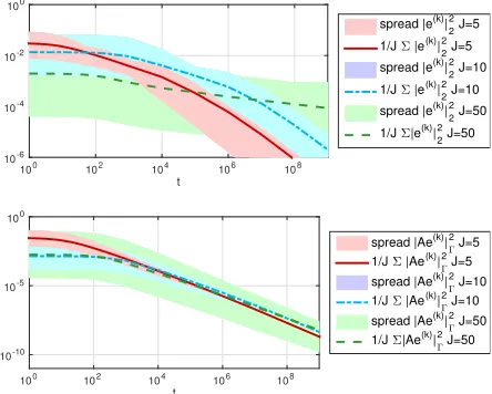
t
100 102 104 106 108
[image:12.612.146.368.357.535.2]10-6 10-4 10-2 100
spread |e(k)| 2 2
J=5
1/J Σ |e(k)| 2 2 J=5
spread |e(k)| 2 2
J=10
1/J Σ |e(k)| 2 2
J=10
spread |e(k)| 2 2
J=50
1/J Σ|e(k)| 2 2
J=50
t
100 102 104 106 108
10-10 10-5 100
spread |Ae(k)|
Γ
2 J=5 1/J Σ |Ae(k)|
Γ
2 J=5
spread |Ae(k)|
Γ
2 J=10 1/J Σ |Ae(k)|
Γ
2 J=10 spread |Ae(k)|
Γ
2 J=50
1/J Σ|Ae(k)|
Γ
2 J=50
Fig. 1. Quantities |e|2
2, |Ae|2Γ w.r. to time t, J = 5
(red), J = 10(blue) and J = 50 (green), β = 10, K =
24−1, initial ensemble chosen based on KL expansion of
C0=β(A−id)−1.
As shown in Theorem3, the rate of convergence of the ensemble collapse is algebraic
(cf. Figure 1) with a constant growing with larger ensemble size. Comparing the
dynamical behavior of the residuals, we observe that, for the ensemble of size J=5, the estimate can be improved in the beginning, but reaches a plateau after a short
time. Increasing the number of particles toJ = 10 improves the accuracy of the
esti-mate. For the ensemble sizeJ = 50, Figure2shows the convergence of the projected
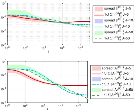
residuals, i.e. the observations can be perfectly recovered. The same behavior can be observed by comparing the EnKF estimate with the truth and the observational data
t
100 102 104 106 108
[image:13.612.145.369.117.300.2]10-3 10-2 10-1 100
spread |r(k)|
2 2
J=5
1/J Σ |r(k)|
2 2
J=5
spread |r(k)|
2 2
J=10
1/J Σ|r(k)|
2 2
J=10
spread |r(k)| 2 2 J=50
1/J Σ|r(k)|22 J=50
t
100 102 104 106 108
10-6 10-4 10-2 100
spread |Ar(k)|
Γ 2
J=5 1/J Σ |Ar(k)|
Γ 2 J=5
spread |Ar(k)|
Γ 2
J=10 1/J Σ |Ar(k)|
Γ 2
J=10
spread |Ar(k)|
Γ 2
J=50 1/J Σ|Ar(k)|
Γ 2
J=50
Fig. 2. Quantities |r|2
2, |Ar|2Γ w.r. to time t,J = 5
(red), J = 10(blue) and J = 50 (green), β = 10, K =
24−1, initial ensemble chosen based on KL expansion of
C0=β(A−id)−1.
The results derived in this paper hold true for each particle, however, for the sake of presentation, the empirical mean of the quantities of interest is shown and the spread indicates the minimum and maximum deviations of the ensemble members from the empirical mean.
t
100 102 104 106 108
10-7
10-6
10-5
10-4
10-3
10-2
10-1
100
101
102
|R|
F J=5
|E|F J=5 |F|
F J=5
|R|F J=10 |E|F J=10 |F|F J=10 |R|F J=50 |E|F J=50 |F|F J=50
Fig. 3. QuantitieskEkF,kFkF, kRkF
w.r. to timet,J= 5(red),J= 10(blue) and
J= 50 (green),β= 10,K= 24−1, initial
ensemble chosen based on KL expansion of
C0=β(A−id)−1.Comparison of the EnKF
t
0 0.5 1 1.5 2 2.5 3 3.5
-0.4 -0.2 0 0.2 0.4 0.6
utruth EnKF est. J=5 EnKF est. J=10 EnKF est. J=50
t
0 0.5 1 1.5 2 2.5 3
0 0.02 0.04 0.06 0.08 0.1 0.12
observations EnKF est. J=5 EnKF est. J=10 EnKF est. J=50
Fig. 4. Comparison of the EnKF
esti-mate with the truth and the observations,J=
5(red), J = 10 (blue) and J = 50(green),
β= 10,K= 24−1, initial ensemble chosen
based on KL expansion ofC0=β(A−id)−1.
Due to the construction of the ensembles in the example, the subspace spanned by the ensemble of size 5 is a strict subset of the subspace spanned by the larger ensembles.
Thus, due to Theorem 4, which characterizes the convergence of the residuals with
respect to the approximation quality of the subspace spanned by the initial ensem-ble, the EnKF estimate can be substantially improved by controlling this subspace.
[image:13.612.112.437.425.559.2]monotonically, but levels off after a short time. Similar convergence properties can
be observed forJ = 10. The same behavior is expected for the larger ensemble, when
integrating over a larger time horizon. This can be also observed for the matrix-valued
quantities depicted in Figure3.
We will investigate this point further by comparing the performance of two en-sembles, both of size 5: one based on the KL expansion and one chosen such that the
contribution ofAr⊥(j)(t) in Theorem 4 is minimized. Since we use artificial data, we
can minimize the contribution ofAr(⊥j)(t) by ensuring thatAr(1)=PJ
k=1αkAe(k)for
some coefficientsαk ∈R. Givenu(2), . . . , u(J) and coefficients α1, . . . , αJ, we define
u(1)= (1−α
1+P
J
k=1αk/J)−1(u†−α1/JP
J j=2 u
(j)+PJ
k=2αku(k)−αk/JP J j=2u
(j)),
which gives the desired property of the ensemble. Note that this approach is not feasible in practice and has to be replaced by an adaptive strategy minimizing the
contribution of Ar⊥(j)(t). However this experiment serves to illusrate the important
role of the initial ensemble in determining the error and is included for this reason. The convergence rate of the mapped residuals and of the ensemble collapse is
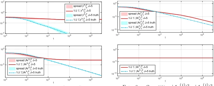
alge-braic in both cases, with rate 1 (in the squared Euclidean norm). Figure 5 shows
the convergence of the projected residuals for the adaptively chosen ensemble. The
decomposition of the residuals (cf. Figure6) numerically verifies the presented theory,
which motivates the adaptive construction of the ensemble. Methods to realize this strategy, in the linear and nonlinear case, will be addressed in a subsequent paper.
t
100 102 104 106 108
10-4 10-2 100 102
spread |rk| 2 2 J=5
1/J Σ |rk|22 J=5 spread |rk|
2 2 J=5 truth
1/J Σ|rk| 2 2 J=5 truth
t
100 102 104 106 108
10-5 100
spread |Ark|
Γ
2 J=5 1/J Σ |Ark|
Γ
2 J=5
spread |Ark|
Γ
2 J=5 truth 1/J Σ|Ark|
Γ
2 J=5 truth
Fig. 5. Quantities |r|2
2, |Ar|2Γ w.r. to
timet,J= 5based on KL expansion ofC0=
β(A−id)−1 (red) andJ= 5minimizing the
contribution ofAr⊥(j)(t)(blue), β= 10,K=
24−1. Comparison of the EnKF estimate
t
100 102 104 106 108
10-10
10-5
100
spread |Ark II|Γ
2 J=5
1/J Σ |Ark II|Γ
2 J=5
spread |Ark II|Γ
2 J=5 truth
1/J Σ |Ark II|Γ
2 J=5 truth
t
100 102 104 106 108
10-10
10-5
100
1/J Σ |Ark
⊥|Γ
2 J=5
1/J Σ |Ark
⊥|Γ
2 J=5 truth
Fig. 6. Quantities |Ark(j)|2 Γ, |Ar
(j) ⊥ |2Γ
w.r. to timet,J= 5based on KL expansion
ofC0 =β(A−id)−1 (red) andJ = 5
min-imizing the contribution of Ar⊥(j)(t) (blue),
β= 10,K= 24−1.
5.1.2. Noisy Observational Data. We will now allow for noise in the
obser-vational data, i.e. we assume that the data is given by y† =OA−1u†+η†, whereη†
is a fixed realization of the random vectorη∼ N(0,0.012id). Note that the standard
deviation is chosen to be roughly 10% of the (maximum of the) observed data. Besides
the quantities e and r, the misfit ϑ(j) =Au(j)−y† = Ar(j)−η† of each ensemble
member is of interest, since, in practice, the residual is not accessible and the misfit is used to check for convergence and to design an appropriate stopping criterion.
Besides the two ensembles with 5 particles introduced in the previous section, we
define an additional one minimizing the contribution ofϑ(⊥j)to the misfit, analogously
[image:14.612.90.439.360.501.2]mo-tivated by the analogue of Theorem 4 in the noisy data case. Note that the design of an adaptive ensemble based on the decomposition of the projected residual is, in
general, not feasible without explicit knowledge of the noiseη†.
t
100 102 104 106 108 1010
10-4
10-3
10-2
[image:15.612.90.441.144.325.2]10-1
spread |rk| 2 2 J=5
[image:15.612.91.437.399.535.2]1/J Σ |rk| 2 2 J=5
spread |rk| 2 2 J=5 truth
1/J Σ|rk| 2 2 J=5 truth
t
100 102 104 106 108 1010
10-2
10-1
100
101
spread |Ark|
Γ
2 J=5
1/J Σ |Ark|
Γ
2 J=5
spread |Ark|
Γ
2 J=5 truth
1/J Σ|Ark|
Γ
2 J=5 truth
Fig. 7.Quantities|r|2
2,|Ar|2Γw.r. tot,
J= 5based on KL expansion ofC0=β(A−
id)−1 (red),J= 5 adaptively chosen (blue),
β= 10,K= 24−1,η∼ N(0,0.012id).
t
100 102 104 106 108
10 12 14 16 18 20 22 24 26 28 30
spread |ϑ|Γ2 J=5 1/J Σ|ϑ|Γ2 J=5 spread |ϑ|
Γ
2 J=5 truth
1/J Σ|ϑ|
Γ
2 J=5 truth
Fig. 8.Misfit|ϑ|2
2w.r. to timet,J= 5
based on KL expansion ofC0=β(A−id)−1
(red), J = 5 adaptively chosen (blue), β =
10,K= 24−1,η∼ N(0,0.012id).
Figure 7 illustrates the well-known overfitting effect, which arises without using
ap-propriate stopping criteria. The method tries to fit the noise in the measurements, which results in an increase in the residuals. This effect is not seen in the misfit
functional, cf. Figure8 and Figure9.
t
100 102 104 106 108 1010
10-8 10-6 10-4 10-2 100 102
1/J Σ|ϑ II|Γ
2 J=5
1/J Σ|ϑ II|Γ
2 J=5 truth
t
100 102 104 106 108 1010
10-4
10-2
100
102
1/J Σ|ϑ ⊥|Γ
2 J=5
1/J Σ|ϑ ⊥|Γ
2 J=5 truth
Fig. 9. Quantities |ϑ(kj)| 2 Γ,|ϑ
(j) ⊥|2Γ w.r.
to time t,J = 5based on KL expansion of
C0 =β(A−id)−1 (red),J = 5 minimizing
the contribution of Ar(⊥j)(t) (blue), β = 10,
K= 24−1,η∼ N(0,0.012id).
t
0 0.5 1 1.5 2 2.5 3 3.5
-0.4 -0.2 0 0.2 0.4 0.6 utruth EnKF est. J=5 EnKF est. J=5 truth
t
0 0.5 1 1.5 2 2.5 3
0 0.02 0.04 0.06 0.08 0.1 0.12 observations EnKF est. J=5 EnKF est. J=5 truth
Fig. 10.Comparison of the EnKF
esti-mate with the truth and the observations,J=
5based on KL expansion ofC0=β(A−id)−1
(red), J = 5 minimizing the contribution
of Ar(⊥j)(t) (blue), β = 10, K = 24 −1,
η∼ N(0,0.012id).
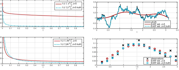
However, the comparison of the EnKF estimates to the truth reveals, in Figure10, the
strong overfitting effect and suggests the need for a stopping criterion. The Bayesian
setting itself provides a so-called a priori stopping rule, i.e. the SMC viewpoint
motivates a stopping of the iterations at timeT = 1. Another common choice in the
deterministic optimization setting is the discrepancy principle, which accounts for the
realization of the noise by checking the following conditionkG(¯u(t))−ykΓ ≤τ, where
t
0 0.1 0.2 0.3 0.4 0.5 0.6 0.7 0.8 0.9 1
0 0.02 0.04 0.06 0.08 0.1 0.12 0.14
1/J Σ |rk|2 2 J=5 1/J Σ|rk|2
2 J=5 truth
t
0 0.1 0.2 0.3 0.4 0.5 0.6 0.7 0.8 0.9 1
0 20 40 60 80 100
1/J Σ |Ark|Γ2 J=5 1/J Σ|Ark|
Γ
[image:16.612.94.439.115.251.2]2 J=5 truth
Fig. 11. Quantities|r|2
2, |Ar|2Γ w.r. to
time t, J = 5 based on KL expansion of
C0 =β(A−id)−1 (red), J = 5 minimizing
the contribution of Ar(⊥j)(t) (blue), β = 10,
K = 24−1, η ∼ N(0,0.012id), Bayesian
stopping rule.J= 5minimizing the
contribu-tion ofAr(j)⊥ (t)(
t
0 0.5 1 1.5 2 2.5 3 3.5
-0.4 -0.2 0 0.2 0.4 0.6 utruth EnKF est. J=5 EnKF est. J=5 truth
t
0 0.5 1 1.5 2 2.5 3
0 0.02 0.04 0.06 0.08 0.1 0.12 observations EnKF est. J=5 EnKF est. J=5 truth
Fig. 12.Comparison of the EnKF
esti-mate with the truth and the observations,J=
5based on KL expansion ofC0=β(A−id)−1
(red), J = 5 minimizing the contribution
of Ar⊥(j)(t) (blue), β = 10, K = 24 −1,
η∼ N(0,0.012id), Bayesian stopping rule.
Figures 11- 12 show the results obtained by employing the Bayesian stopping rule,
i.e. by integrating up to timeT = 1. The adaptively chosen ensemble leads to much
better results in the case of the Bayesian stopping rule. Since we do not expect to have explicit knowledge of the noise, the adaptive strategy as presented above is in general not feasible. However an adaptive choice of the ensemble according to the
misfit may lead to a strong overfitting effect, as shown in Figures13-14.
t
100 102 104 106 108
[image:16.612.141.434.438.573.2]10-16 10-14 10-12 10-10 10-8 10-6 10-4 10-2 100 102
spread |ϑ|Γ2 J=5
1/J Σ|ϑ|Γ2 J=5 spread |ϑ|Γ2 J=5 truth
1/J Σ|ϑ|
Γ
2 J=5 truth
spread |ϑ|Γ2 J=5 truth mis.
1/J Σ|ϑ|
Γ
2 J=5 truth mis.
Fig. 13.Misfit|ϑ|2
Γw.r. to timet,J= 5
based on KL expansion ofC0=β(A−id)−1
(red),J= 5adaptively chosen (blue),J= 5
minimizing the contribution of ϑ⊥ w.r. to
misfit (gray), β = 10, K = 24 −1, η ∼
N(0,0.012id).
t
0 0.5 1 1.5 2 2.5 3 3.5
-1 -0.5 0 0.5 1 utruth EnKF est. J=5 EnKF est. J=5 truth EnKF est. J=5 truth mis.
t
0 0.5 1 1.5 2 2.5 3
0 0.02 0.04 0.06 0.08 0.1 0.12 observations EnKF est. J=5 EnKF est. J=5 truth EnKF est. J=5 truth mis.
Fig. 14. Comparison of the EnKF
es-timate with the truth and the observations,
J = 5 based on KL expansion of C0 =
β(A−id)−1 (red), J = 5adaptively chosen
(blue),J= 5minimizing the contribution of
ϑ⊥w.r. to misfit (gray),β= 10,K= 24−1,
The overfitting effect is still present in the small noise regime as shown below. The
standard deviation of the noise is reduced by 100, i.e. η ∼ N(0,0.0012id).
t
100 102 104 106 108
[image:17.612.90.438.148.287.2]10-16 10-14 10-12 10-10 10-8 10-6 10-4 10-2 100 102
spread |ϑ|
Γ
2 J=5
1/J Σ|ϑ|
Γ
2 J=5
spread |ϑ|
Γ
2 J=5 truth
1/J Σ|ϑ|Γ2 J=5 truth
spread |ϑ|
Γ
2 J=5 truth mis.
1/J Σ|ϑ|Γ2 J=5 truth mis.
Fig. 15.Misfit|ϑ|2
Γw.r. to timet,J= 5
based on KL expansion ofC0=β(A−id)−1
(red),J= 5adaptively chosen (blue),J= 5
minimizing the contribution of ϑ⊥ w.r. to
misfit (gray), β = 10, K = 24 −1, η ∼
N(0,0.0012id).
t
0 0.5 1 1.5 2 2.5 3 3.5
-1 -0.5 0 0.5 1
utruth EnKF est. J=5 EnKF est. J=5 truth EnKF est. J=5 truth mis.
t
0 0.5 1 1.5 2 2.5 3
0 0.02 0.04 0.06 0.08 0.1 0.12
observations EnKF est. J=5 EnKF est. J=5 truth EnKF est. J=5 truth mis.
Fig. 16. Comparison of the EnKF es-timate with the truth and the observations,
J = 5 based on KL expansion of C0 =
β(A−id)−1 (red), J = 5adaptively chosen
(blue),J= 5minimizing the contribution of
ϑ⊥w.r. to misfit (gray),β= 10,K= 24−1,
η∼ N(0,0.0012id).
The ill-posedness of the problem leads to the instabilities of the identification problem and requires the use of an appropriate stopping rule.
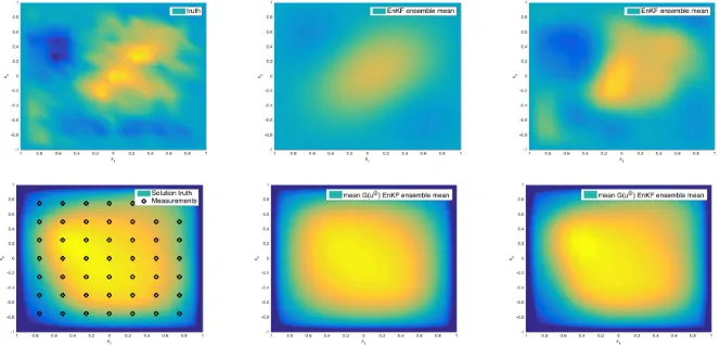
5.2. Nonlinear Forward Model. To investigate the numerical behavior of the EnKF for nonlinear inverse problems, we consider the following two-dimensional el-liptic PDE:
−div(eu∇p) =f inD:= (−1,1)2, p= 0 in ∂D.
We aim to find the log permeability u from 49 observations of the solution p on
a uniform grid in D. We choose f(x) = 100 for the experiments. The mapping
from uto these observations is now nonlinear. Again we work in the noise-free case,
and take Γ = I, Σ = 0 and solve (6) to estimate the unknown parameters. The
prior is assumed to be Gaussian with covariance operator C0 = (−4)−2, employing
homogeneous Dirichlet boundary conditions to define the inverse of −4. We use
a FEM approximation based on continuous, piecewise linear ansatz functions on a
uniform mesh with meshwidthh= 2−4. The initial ensemble of size 5 and 50 is chosen
based on the KL expansion ofC0 in the same way as in the previous subsection.
The results given in Figure 17 and Figure 18show a similar behavior as in the
linear case. The approximation quality of the subspace spanned by the initial ensemble clearly influences, also in the nonlinear example, the accuracy of the estimate. Taking a look at the EnKF estimate in this nonlinear setting, we observe a satisfactory approximation of the truth and a perfect match of the observational data in the case
t
100 102 104 106 108
10-5 100
spread |ek| 2 2 J=5
1/JΣ |ek| 2 2 J=5
spread |ek| 2 2 J=50
1/JΣ |ek|22 J=50
t
100 102 104 106 108
10-10 10-5
spread |G(uk)-1/J Σ G(uj)|
Γ
2 J=5
1/JΣ |G(uk)-1/J
Σ G(uj)|
Γ
2 J=5
spread |G(uk)-1/J Σ G(uj)|
Γ
2 J=50
1/JΣ |G(uk)-1/J
Σ G(uj)|
Γ
[image:18.612.91.442.107.245.2]2 J=50
Fig. 17. Quantities|e(k)|2
2, |G(u(k))− 1
J
PJ
j=1G(u(j)|2Γ w.r. to timet,J= 5(red)
andJ = 50(green), initial ensemble chosen
based on KL expansion ofC0= (−4)−2.
t
100 102 104 106 108
10-6 10-4 10-2 100
spread |rk| 2 2 J=5
1/JΣ |rk| 2 2 J=5
spread |rk| 2 2 J=50
1/JΣ |rk| 2 2 J=50
t
100 102 104 106 108
10-2 100 102 104
spread |G(uk)-G(u+)|
Γ
2 J=5
1/JΣ|G(uk)-G(u+)|
Γ
2 J=5
spread |G(uk)-G(u+)|
Γ
2 J=50
1/JΣ|G(uk)-G(u+)|
Γ
[image:18.612.89.421.313.472.2]2 J=50
Fig. 18. Quantities |r(k)|2
2 |G(u(k))−
G(u†)|2
Γw.r. to timet,J= 5(red) andJ=
50(green), initial ensemble chosen based on
KL expansion ofC0= (−4)−2.
Fig. 19. Comparison of the truth (left above) and the EnKF estimate w.r. tox, J=5 (middle
above) ,J = 50(right above) and comparison of the forward solutionG(u†) (left below) and the
estimated solutions of the forward problemJ= 5(middle below),J= 50(right below).
6. Variants on EnKF. In this section we describe three variants on the EnKF, all formulated in continuous time in order to facilitate comparison with the preceding studies of the standard EnKF in continuous time. The first two methods, variance inflation and localization, are commonly used by practitioners in both the filtering
and inverse problem scenarios [8,1]. The third method, random search, is motivated
by the SMC derivation of the EnKF for inverse problems, and is new in the context of the EnKF. For all three methods we provide numerical results which illustrate the behavior of the EnKF variant, in comparison with the standard method. In the following, we focus on the linear case with Σ = 0. The methods from the first two subsections have generalizations in the general nonlinear setting, and indeed are widely used in data assimilation and, to some extent, in geophysical inverse problems; but
The method in the final subsection is implemented through an entirely derivative-free MCMC method, and is hence automatically defined, as is, for nonlinear as well as linear inverse problems.
6.1. Variance Inflation. The empirical covariancesCupandCpp all have rank
no greater thanJ−1 and hence are rank deficient whenever the number of particles
J is less than the dimension of the spaceX. Variance inflation proceeds by correcting
such rank deficiencies by the addition of self-adjoint, strictly positive operators. A
natural variance inflation technique is to add a multiple of the prior covarianceC0to
the empirical covariance which gives rise to the equations
(15) du
(j)
dt =− αC0+C(u)
DuΦ(u(j);y), j = 1, . . . , J ,
where Φ is as defined in (10). Taking the inner-product in X withDuΦ(u(j);y) we
deduce that
dΦ(u(j);y)
dt ≤ −αkC
1 2
0DuΦ(u(j);y)k2,
This implies that all ω−limit points of the dynamics are contained in the critical
points of Φ(·;y).
6.2. Localization. Localization techniques aim to remove spurious long
dis-tance correlations by modifying the covariance operators Cup and Cpp, or directly
the Kalman gain Cnup+1(Cnpp+1+h−1Γ)−1. Typical convolution kernels reducing the
influence of distant regions are of the form
ρ:D×D→R
ρ(x, y) = exp(−|x−y|r),
where D⊂Rd, d∈Ndenotes the physical domain and| · |is a suitable norm in D,
r∈N, cf. [21]. The continuous time limit in the linear setting then reads as
(16) du
(j)
dt =−C
loc
(u)DuΦ(u(j);y), j= 1, . . . , J ,
whereCloc(u)φ(x) =R
Dφ(y)k(x, y)ρ(x, y)dy withkdenoting the kernel ofC(u) and
φ∈ X.
6.3. Randomized Search. We notice that the mapping on probability
mea-sures given by (3) may be replaced by
µn+1=LnPnµn.
wherePnis any Markov kernel which preservesµn.For example we may takePnto be
the pCN method [6] for measure µn. One step of the pCN method for given particle
u(nj)in iterationnis realized by
• Proposevn(j)=
p
(1−β2)u(j)
n +βι(j), ι(j)∼ N(0, C0).
• Set ˜u(nj)=v
(j)
n with probability a(u
(j)
n , v
(j)
n ).
• Set ˜u(nj)=u
(j)
n otherwise
assuming the prior is Gaussian, i.e. N(0, C0). The acceptance probability is given by
The particles ˜u(nj) are used to approximate the measure ˜µn = Pnµn, which is then
mapped toµn+1by the application of Bayes’ theorem, i.e. µn+1=Lnµ˜n.
Using the continuous-time diffusion limit arguments from [26, Theorem 4], which
apply in the nonlinear case, and combining with the continuous time limits described for the EnKF earlier in this paper, we obtain
du(j)
dt =
1 J
J
X
k=1
G(u(k))− G, y− G(u(j))
Γ u (k)
−u
−u(j)−tC0DuΦ(u(j);y) +
p
2C0
dW(j)
dt .
(17)
Although the limiting equation involves gradients of Φ, and hence adjoints for the for-ward model, the discrete time implementation above avoids the gradient computation by using the accept-reject step, and remains a derivative free optimizer.
6.4. Numerical Results. In the following, to illustrate behavior of the EnKF variants, we present numerical experiments for the linear forward problem in the
noise-free case: (13) and (14) withη = 0. The performance of the EnKF variants is
compared to the basic algorithms shown in Figure2and Figure4.
6.4.1. Inflation. We investigate the numerical behavior of variance inflation of
the form given in (15) with α = 0.01. Figures 20 and 21 show that the variance
inflated method becomes a preconditioned gradient flow, which, in the linear case, leads to fast convergence of the projected iterates. It is noteworthy that in this case there is very little difference in behavior between ensemble sizes of 5 and 50.
t
100 102 104 106 108
10-3
10-2
10-1
100
101
102
spread |rk| 2 2 J=5 VI
1/J Σ |rk| 2 2 J=5 VI
spread |rk|22 J=50 VI
1/J Σ|rk| 2 2 J=50 VI
t
100 102 104 106 108
10-6
10-4
10-2
100
spread |Ark|
Γ
2 J=5 VI
1/J Σ |Ark|
Γ
2 J=5 VI
spread |Ark|
Γ
2 J=50 VI
1/J Σ|Ark|
Γ
[image:20.612.135.369.171.222.2]2 J=50
Fig. 20. Quantities|r|2
2, |Ar|2Γ w.r. to
timet, J = 5 with variance inflation (red)
and J = 50with variance inflation (green),
β= 10,K= 24−1, initial ensemble chosen
based on KL expansion ofC0=β(A−id)−1.
Comparison of the EnKF
t
0 0.5 1 1.5 2 2.5 3 3.5
-0.6 -0.4 -0.2 0 0.2 0.4
utruth EnKF est. J=5 VI EnKF est. J=50 VI EnKF est. J=5 orig. EnKF est. J=50 orig.
t
0 0.5 1 1.5 2 2.5 3
0 0.02 0.04 0.06 0.08 0.1 0.12
observations EnKF est. J=5 VI EnKF est. J=50 VI
Fig. 21. Comparison of the EnKF es-timate with the truth and the observations,
J= 5with variance inflation (red) and J=
50with variance inflation (green), β = 10,
K= 24−1, initial ensemble chosen based on
KL expansion ofC0=β(A−id)−1.
6.4.2. Localization. We consider a localization of the form given by equations
(16), (16) with r = 2 and Euclidean norm inside the cut-off kernel. Figures 22
-23 clearly demonstrate the improvement by the localization technique, which can
[image:20.612.91.434.425.560.2]t
100 102 104 106 108
10-3
10-2
10-1
100
101
102
spread |rk| 2 2 J=5 loc
1/J Σ |rk| 2 2 J=5 loc
spread |rk| 2 2 J=50 loc
1/J Σ|rk|22 J=50 loc
t
100 102 104 106 108
10-6
10-4
10-2
100
spread |Ark|
Γ
2 J=5 loc
1/J Σ |Ark|
Γ
2 J=5 loc
spread |Ark|Γ2 J=50 loc 1/J Σ|Ark|
Γ
2 J=50
Fig. 22. Quantities|r|2
2, |Ar|2Γ w.r. to
timet,J= 5with localization (red) andJ=
50 with localization (green), β = 10, K =
24−1, initial ensemble chosen based on KL
expansion ofC0=β(A−id)−1. Comparison
of the EnKF
t
0 0.5 1 1.5 2 2.5 3 3.5
-0.6 -0.4 -0.2 0 0.2 0.4
utruth EnKF est. J=5 loc EnKF est. J=50 loc EnKF est. J=5 orig. EnKF est. J=50 orig.
t
0 0.5 1 1.5 2 2.5 3
0 0.02 0.04 0.06 0.08 0.1 0.12
[image:21.612.90.439.119.254.2]observations EnKF est. J=5 loc EnKF est. J=50 loc
Fig. 23. Comparison of the EnKF es-timate with the truth and the observations,
J= 5with localization (red) andJ= 50with
localization (green),β= 10,K= 24−1,
ini-tial ensemble chosen based on KL expansion
ofC0=β(A−id)−1.
6.4.3. Randomized Search. We investigate the behavior of randomized search
for the linear problem withG(·) =A·. For the numerical solution of the continuous
limit (17), we employ a splitting scheme with a linearly implicit Euler step, namely
˜
u(nj+1) =√1−2hu(nj)+p2hC0ζn
Kun(j+1) = ˜un(j+1) +h(C(˜un+1)A∗Γ−1y†+nhC0A∗Γ−1y†),
where ζn ∼ N(0, id) and K := I+h(C(˜un+1)A∗Γ−1A+nhC0A∗Γ−1A). In all
nu-merical experiments reported we take h= 2−8. Figure24 and Figure 25show that
the randomized search leads to an improved performance compared to the original EnKF method. Due to the fixed step size and the resulting high computational costs,
the solution is computed up to time T = 100. In order to accelerate the numerical
solution of the limit (17), implicit schemes can be considered. Note that the limit
requires the computation of the gradients, which is in practice undesirable. However, the limit reveals from a theoretical point of view important structure, whereas the discrete version is more suitable for applications. The advantage of the randomized search is apparent.
6.4.4. Summary. The experiments show a similar performance for all discussed variants. The variance inflation technique and the localization variant both lead to gradient flows, which are, in the noise-free case, favorable due to the fast convergence. On the other hand, these strategies also accelerate the convergence of the ensemble to the mean (ensemble collapse) and may be considered less desirable for this reason. The randomized search preserves by construction the spread of the ensemble. A similar
regularization effect is achieved by perturbing the observational data, see (6). The
t
100 102 104 106 108
10-3
10-2
10-1
100
101
102
spread |rk| 2 2 J=5 MM 1/J Σ |rk|
2 2 J=5 MM spread |rk|
2 2 J=50 MM 1/J Σ|rk|
2 2 J=50 MM
t
100 102 104 106 108
10-6
10-4
10-2
100
spread |Ark|
Γ
2 J=5 MM 1/J Σ |Ark|
Γ
2 J=5 MM spread |Ark|
Γ
2 J=50 MM 1/J Σ|Ark|
Γ
2 J=50
Fig. 24. Quantities|r|2
2, |Ar|2Γ w.r. to
timet,J = 5 with randomized search (red)
andJ = 50with randomized search (green),
β= 10,K= 24−1, initial ensemble chosen
based on KL expansion ofC0=β(A−id)−1.
Comparison of the EnKF
t
0 0.5 1 1.5 2 2.5 3 3.5
-0.6 -0.4 -0.2 0 0.2 0.4
utruth EnKF est. J=5 MM EnKF est. J=50 MM EnKF est. J=5 orig. T=100 EnKF est. J=50 orig. T=100
t
0 0.5 1 1.5 2 2.5 3
0 0.02 0.04 0.06 0.08 0.1 0.12
[image:22.612.102.438.108.242.2]observations EnKF est. J=5 MM EnKF est. J=50 MM
Fig. 25. Comparison of the EnKF es-timate with the truth and the observations,
J= 5with randomized search (red) andJ=
50with randomized search (green),β = 10,
K= 24−1, initial ensemble chosen based on
KL expansion ofC0=β(A−id)−1.
We study the same test case as in section5.1.2, with the same realization of the
measurement noise (cf. Figure 11 and Figure 12), to allow for a comparison of the
three methods introduced in this section. Combining the various techniques with the Bayesian stopping rule for noisy observations, we observe the following behavior given
in Figure26and Figure27.
t
0 0.2 0.4 0.6 0.8 1 0.02
0.04 0.06 0.08 0.1 0.12 0.14
1/J Σ |rk| 2 2 J=5 VI
1/J Σ |rk| 2 2 J=5 loc
1/J Σ |rk| 2 2 J=5 MM
t
0 0.2 0.4 0.6 0.8 1 5
10 15 20 25 30
1/J Σ |Ark| Γ
2 J=5 VI 1/J Σ |Ark|
Γ
2 J=5 loc
1/J Σ |Ark| Γ
[image:22.612.119.395.393.617.2]2 J=5 MM
Fig. 26. Quantities|r|2
2,|Ar|2Γw.r. to timet,J= 5(red) for the discussed variants,β= 10,
β= 10,K= 24−1, initial ensemble chosen based on KL expansion ofC0=β(A−id)−1.
better estimate of the unknown data. In Figures26and27, one path of the solution
of (17) is shown, similar performance can be observed for further paths. This strategy
has the potential to significantly improve the performance of the EnKF and will be investigated in more details in subsequent papers.
t
0 0.5 1 1.5 2 2.5 3 3.5 -0.4
-0.2 0 0.2 0.4 0.6
utruth
EnKF est. J=5 VI EnKF est. J=5 loc EnKF est. J=5 MM EnKF est. J=5 orig.
t
0 0.5 1 1.5 2 2.5 3
0 0.02 0.04 0.06 0.08 0.1 0.12
[image:23.612.117.396.166.391.2]observations EnKF est. J=5 VI EnKF est. J=5 loc EnKF est. J=5 MM
Fig. 27. Comparison of the EnKF estimate with the truth and the observations,J = 5(red)
for the discussed variants,β= 10,K= 24−1, initial ensemble chosen based on KL expansion of
C0=β(A−id)−1.
7. Conclusions. Our analysis and numerical studies for the ensemble Kalman filter applied to inverse problems demonstrate several interesting properties: (i) the continuous time limit exhibits structure that is hard to see in discrete time implemen-tations used in practice; (ii) in particular, for the linear inverse problem, it reveals an underlying gradient flow structure; (iii) in the linear noise-free case the method can be completely analyzed and this leads to a complete understanding of error propaga-tion; (iv) numerical results indicate that the conclusions observed for linear problems carry over to nonlinear problems; (v) that the widely used localization and inflation techniques can improve the method, but that the (introduced here for the first time) use of ideas from SMC hold considerable promise for further improvement; (vi) that importing stopping criteria and other regularization techniques is crucial to the
ef-fectiveness of the method, as highlighted by the work of Iglesias [14,16]. Our future
work in this area, both theoretical and computational, will reflect, and build on, these conclusions.