Risk Return Relationship in the Portfolio Selection Models

http://www.scirp.org/journal/tel ISSN Online: 2162-2086

ISSN Print: 2162-2078

DOI: 10.4236/tel.2018.83025 Feb. 12, 2018 358 Theoretical Economics Letters

Risk Return Relationship in the Portfolio

Selection Models

Ken Hung

, C. W. Yang

, Yifan Zhao

, Kuo-Hao Lee

1_{Texas A & M International University, Laredo, TX, USA} 2_{Clarion University of Pennsylvania, Clarion, PA, USA}

3_{Department of Finance, Zeigler College of Business, Bloomsburg University of Pennsylvania, Bloomsburg, PA, USA}

Abstract

In this paper, we calculate four different kinds of means—AM, GM, HM, and GDM—to investigate the risk-return contour using Markowitz risk minimiza-tion and Sharpe’s angle maximizaminimiza-tion models. For a given k value (target portfolio return), the rank order of risk or variance-covariance (υ) can change. In the vertical segment of an efficient frontier curve, we observed v(GDM) > v(HM) > v(GM) > v(AM). At higher k values, the rank changes to v(GDM) > v(HM) > v(AM) > v(GM). That is to say, ranking a portfolio using different kinds of means may well give different rankings depending on what

k value one is evaluating. It is also shown the harmonic mean should not be used in the case of a small negative growth rate in stock prices.

Keywords

Arithmetic Mean, Geometric Mean, Golden Mean, Harmonic Mean, Markowitz Risk Minimization, Sharpe’s Angle Maximization

1. Introduction and Literature Reviews

The foundation of modern investment theory is laid upon the quadratic pro-gram portfolio selection model developed more than half century ago by Harry Markowitz [1] [2] [3]. The optimization (risk-minimization) process over mean- variance-covariance space can trace out the efficient frontier curve, which pro-vides the solution space for investors. However, an exact solution cannot be found without the knowledge of a risk free rate on a government bond and an investor’s attitude toward risk. To this end, Sharpe [4] formulated and solved the angle-maximization model in which the risk (standard deviation) adjusted port-How to cite this paper: Hung, K., Yang,

C.W., Zhao, Y.F. and Lee, K.-H. (2018) Risk Return Relationship in the Portfolio Selec-tion Models. Theoretical Economics Letters, 8, 358-366.

https://doi.org/10.4236/tel.2018.83025

Received: October 12, 2017 Accepted: February 9, 2018 Published: February 12, 2018

Copyright © 2018 by authors and Scientific Research Publishing Inc. This work is licensed under the Creative Commons Attribution International License (CC BY 4.0).

http://creativecommons.org/licenses/by/4.0/

DOI: 10.4236/tel.2018.83025 359 Theoretical Economics Letters folio return (net of risk free rate) was maximized. The Sharpe model provides a convex combination of risk free government bonds and a portfolio of stocks se-lected based on the criterion of risk minimization. Attitude toward risk such as 20% on bond and 80% on stocks will give investor an exact solution without the knowledge of the indifference (isoutility) curve. Soto and Su [5] proposed a “sparse” estimator of the inverse covariance matrix that achieves significant out- of-sample risk reduction and improves certainty equivalent returns after trans-action costs. Yang et al.[6] proved that Markowitz risk minimization and Sharpe angle-maximization models are mathematically equivalent given some required portfolio returns and risk free bond rate. Gil-Bazo [7] found the return dynamics is related to the investor’s portfolio choice for different investment horizons and that return predictability under stationarity which may induce both positive and negative horizon effects in the optimal allocation to the risky asset. Best and Grauer [8] investigated and revealed when only a budget constraint is imposed on the investment problem, the analytical results indicate that an MV-efficient portfolio’s weights, mean, and variance can be extremely sensitive to changes in asset means.

Does the choice of mean returns of stocks in the portfolio matter in the selec-tion process? If so, how different are the optimum soluselec-tion sets? In this note, we first apply the well-known means: arithmetic, geometric and harmonic means to five companies stocks. In addition, we add a golden mean to the simulation for comparison. The organization of the paper is as follows. Next section introduces the Markowitz risk minimization and Sharpe angle maximization models. Sec-tion III describes data and four different means. SecSec-tion IV performs computer simulations via LINGO [9] to trace out corresponding efficient frontier curves. Section V gives a conclusion.

2. Portfolio Selection Models with Different Means

Given a set of n selectable stocks, the purpose of the Markowitz portfolio model is to minimize the weighted risk in terms of variance and covariance of n stock returns, or

Minimize 2 2

i i i j ij

i i i j

x x x

υ σ σ

≠

=

∑

∑∑

Subject to i i i

x R ≥k

∑

1

i i

x =

∑

0

i

x ≥ (4)

where xi = the weight or proportion of investment in stock i;

2

i

σ

ij

σ _{= covariance of return between stock i and j;}

i

R = expected or average rate of return of stock i;

DOI: 10.4236/tel.2018.83025 360 Theoretical Economics Letters Note that rate of return is frequently calculated as 1

1 t t t P P P − − −

on which mean,

variance and covariance are calculated. Optimum weights ( * * * 1, 2, , n x x  x ) for

* 0

i

x ≥ are the framework under which weighted risk υ can be calculated. Along

with a set of k values, we have geometric means calculated according to the growth rate formula (next section) and a set of risk-return values on which an efficient frontier curve can be traced.

However, the exact location cannot be determined with a risk-free bond rate

F

R . To expand to risk minimization model, Sharpe [4] proposed an angle-

maximizing model with a highest straight line from RF that is tangent to the

efficient frontier derived from the Markowitz model.

Maximize

(

)

2 2

tan

i i F

i

i i i j ij

i i j

x R R

x x x

θ σ σ − =   +    

∑

∑

∑∑

Subject to _i 1

i x =

∑

0

i

x ≥ (7)

As is shown by Yang et al. [6], a given RF corresponds to a k value in

equa-tion (2) of the Markowitz model. Furthermore, the denominaequa-tion of Equaequa-tion (5) is the square root of the objective function of Equation (1). Thus, the Mar-kowitz and Sharpe models exhibit reciprocal relations for a given set of Ri, RF

and k value.

3. Description of Data and Characteristics of Different Mean

Returns

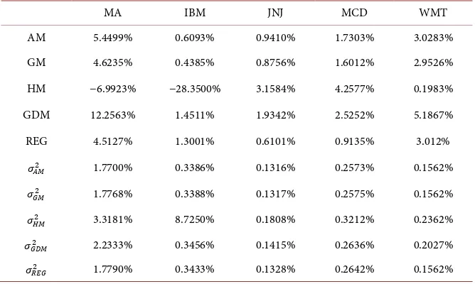
Monthly stock price of 5 companies, Mastercard Incorporated (MA), Interna-tional Business Machines Corp. (IBM), Johnson & Johnson (JNJ), McDonald’s Corp. (MCD), Wal-Mart Stores Inc. (WMT), from September of 2007 to August of 2008 are calculated to obtain 55 (11*5) rates of return [10]. The arithmetic means (AM) and associated variance and covariance of stock returns are re-ported in Table 1.

An examination on five arithmetic means indicates the highest return is by Masters Charge (MA), followed by Wal-Mart (WMT), McDonalds (MCD), Johnson & Johnson (JNJ) and International Business Machine (IBM). As an al-ternative to arithmetic mean is the often used geometric mean:

1 1

3

2 4

1 2 3 1 1

1 1

n n

n n

n

P P P

P P

P P P P− P

   

⋅ ⋅ ⋅⋅⋅ − = −

   

 

  . Note that when

1

i

i P

P

+ _{exceeds (falls short}

of) one it implies a position (negative) growth rate as is measured by

1 1

1

i i i

i i

P P P

P P

+ _{− =} + − _{. Viewed in this light, an arithmetic mean (AM) is derived}

DOI: 10.4236/tel.2018.83025 361 Theoretical Economics Letters

Table 1. Means (%) and variances (%) of five stock returns.

MA IBM JNJ MCD WMT

AM 5.4499% 0.6093% 0.9410% 1.7303% 3.0283%

GM 4.6235% 0.4385% 0.8756% 1.6012% 2.9526%

HM −6.9923% −28.3500% 3.1584% 4.2577% 0.1983%

GDM 12.2563% 1.4511% 1.9342% 2.5252% 5.1867%

REG 4.5127% 1.3001% 0.6101% 0.9135% 3.012%

𝜎𝜎𝐴𝐴𝐴𝐴2 1.7700% 0.3386% 0.1316% 0.2573% 0.1562%

𝜎𝜎𝐺𝐺𝐴𝐴2 1.7768% 0.3388% 0.1317% 0.2575% 0.1562%

𝜎𝜎𝐻𝐻𝐴𝐴2 3.3181% 8.7250% 0.1808% 0.3212% 0.2362%

𝜎𝜎𝐺𝐺𝐺𝐺𝐴𝐴2 2.2333% 0.3456% 0.1415% 0.2636% 0.2027%

𝜎𝜎𝑅𝑅𝑅𝑅𝐺𝐺2 1.7790% 0.3433% 0.1328% 0.2642% 0.1562%

AM = arithmetic mean; GM = geometric mean; HM = harmonic mean; GDM = golden mean; REG =

re-gression-based mean; 2

AM

σ = variance of stock returns using AM as the central location; MA = Mastercard

Incorporated; IBM = International Business Machines Corp; JNJ = Johnson & Johnson; MCD = McDo-nald’s Corp.; WMT = Wal-Mart Stores Inc.

the same measure of rate of return, 1 1

i

i P

P

+ _{− . Well-known in statistics, AM is}

more sensitive to outliers than is GM and as such GM may be preferred in such cases. During the sample period, the five stock prices underwent substantial changes. For example, the greatest monthly price change was 28.4% while the largest drop registered 13.97% for Masters Charge. From the perspective of risk averseness, AM might not be preferred. Calculated geometric mean returns fol-low the same rank order as that of arithmetic mean returns (Table 1).

A harmonic mean may be appropriate for a variable that measures rates of change (e.g., velocity). In business applications, number of shares of stocks of a national fund, a unit of price (e.g., $1,000,000) can purchase could fit into this

category. The harmonic mean (HM) is calculated as 1

1 1

HM

n

i xi n

=

=

∑

represents rate of return for stock i. For n = 2 and xi>0, the geometric mean is the square root of arithmetic and harmonic means or 2

GM =AM HM⋅ . For a

set of clustered numbers, the three means produce very similar values. However, HM can be very biased toward a negative value in the presence of a small negative return, i.e., xi= −0.02 implies

1 50

i

x = − which will dominate other

positive regular returns. This is the case we encounter in calculating HM for IBM and MA (e.g., x11= −0.66% for MA and x4= −0.91% for IBM). For comparison, we report the HM return in Table 1 as well.

DOI: 10.4236/tel.2018.83025 362 Theoretical Economics Letters A location B between points A and C such as AC AB

AB = BC which leads to the

solution 1 5 0.618034 2

− + ₌

. In another word, it is the range (xmax−xmin) that determines the value of golden mean (GDM) since it is hinged calculated as

(

)

min 0.618034 max min

x + ∗ x −x . For instance, the GDM return for MA is

(

)

(

)

13.97% 0.618034

28.47%

13.97%

12.256%

−

+

∗

− −

=

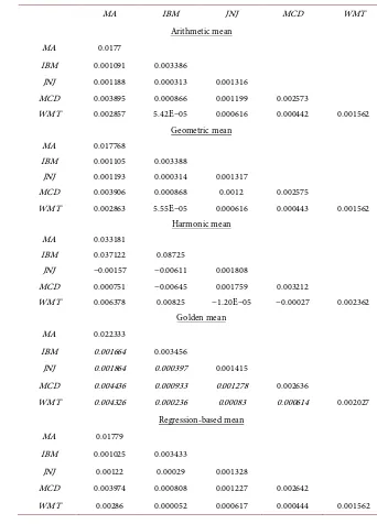
key role in determining a representative value, GDM may be a viable candidate and are reported in Table 1. The corresponding variances and covariances of stock returns using the AM, GM, HM, and GDM are shown in Table 2.

Table 2. Variance and covariance using five means.

MA IBM JNJ MCD WMT

Arithmetic mean

MA 0.0177

IBM 0.001091 0.003386

JNJ 0.001188 0.000313 0.001316

MCD 0.003895 0.000866 0.001199 0.002573

WMT 0.002857 5.42E−05 0.000616 0.000442 0.001562 Geometric mean

MA 0.017768

IBM 0.001105 0.003388

JNJ 0.001193 0.000314 0.001317

MCD 0.003906 0.000868 0.0012 0.002575

WMT 0.002863 5.55E−05 0.000616 0.000443 0.001562 Harmonic mean

MA 0.033181

IBM 0.037122 0.08725

JNJ −0.00157 −0.00611 0.001808

MCD 0.000751 −0.00645 0.001759 0.003212

WMT 0.006378 0.00825 −1.20E−05 −0.00027 0.002362 Golden mean

MA 0.022333

IBM 0.001664 0.003456

JNJ 0.001864 0.000397 0.001415

MCD 0.004436 0.000933 0.001278 0.002636

WMT 0.004326 0.000236 0.00083 0.000614 0.002027 Regression-based mean

MA 0.01779

IBM 0.001025 0.003433

JNJ 0.00122 0.00029 0.001328

MCD 0.003974 0.000808 0.001227 0.002642

DOI: 10.4236/tel.2018.83025 363 Theoretical Economics Letters

4. A Comparison of Simulation Results

An efficient frontier generally consists of two parts: a vertical section and a con-cave part. The vertical part indicates Equation (2) holds with strict inequality (> k). That is the portfolio return at optimality exceeds the minimum required rate

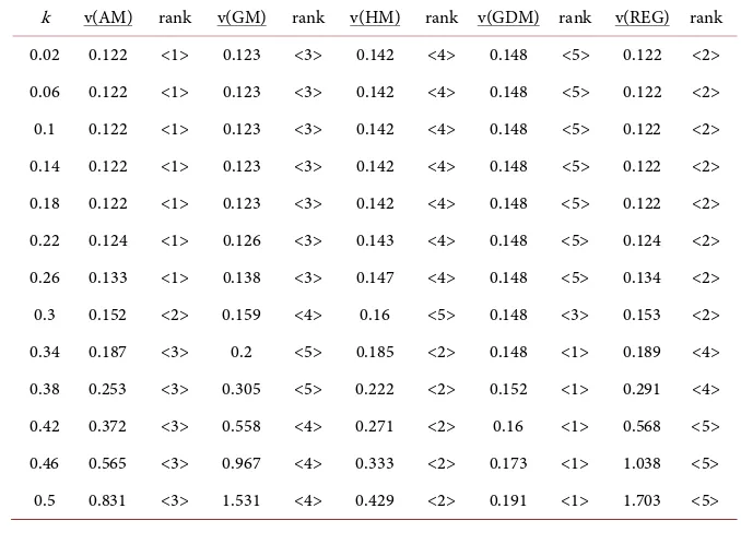
k. For k = 2% (annualized), which is obviously too low. The optimum portfolio return far exceeds k = 2% in the case of AM. If we arbitrarily impose Equation (2) with an equality sign (k = 2%), there will exist no feasible solution, for the lowest annual average rate of return is 7.317% (IBM), and as such the vertical sections of the efficient frontier curve starts to bend at k ≈ _{20%, k = 19%, k =} 18%, and k = 31% in the cases of AM, GM, HM and GDM respectively (Table 3). A perusal of Table 3 indicates that for range of k < 18%, the portfolio risks in the Markowitz model manifest the following rank order 0.1225 (AM) < 0.1226 (GM) < 0.1421 (HM) < 0.1481 (GDM) for each given k value.

As far as minimum risk level where efficient frontier is vertical is concerned, the risk levels of GM and HM are bounded by that AM curve and GDM. Given that GDM are highest in all four means, its variance-covariance is greatest at lower level of k values. The variances of HM are even greater because of negative mean returns. However, five of ten covariances in HM are negative and thus the portfolio risk could be reduced from proper diversification. The high values of the GDM returns translate into higher variances and covariances when com-pared to that of AM and GM. It is little wonder that the efficient frontier has the largest risk in the vertical segment or v(GDM) > v(HM) > v(GM) > v(AM). As k

value increases to 30% the risk become the greatest for HM that has 5 largest va-riances of all the four means. The rank of the portfolio risk become v(HM) > v(GM) > v(AM) > v(GDM). Note that v(GDM) is still at its vertical segment at

Table 3. Risk-return combination using five means.

DOI: 10.4236/tel.2018.83025 364 Theoretical Economics Letters

k = 0.30% (see Table 3).

From k≥0.34 and on the risk in the case of GM become the greatest

be-cause the choice set has dwindled: only WMT (35.436%) and MA (55.477%) have the mean return greater than 34% and as such most of the weights go to WMT and MA regardless of their risk levels. On the contrary risk of GDM as-sumes its smallest value since most of the five stocks have higher returns: 147%, 22.24%, 30.3%, 23.208% and 17.412% for MA, WMT, MCD, JNJ and IBM re-spectively. HM has shown smallest risk due to negative covariance. However, it must be pointed out that small negative returns are biased and misleading in the sense that the double reciprocity formula assigns too much weight to small neg-ative return (slight price decrease in stock). The risk associated with AM for

34%

k≥ is slightly less than that of GM since GM is less sensitive to outliers than is AM, and as such AM has a slightly larger choice set (smaller risk) at high

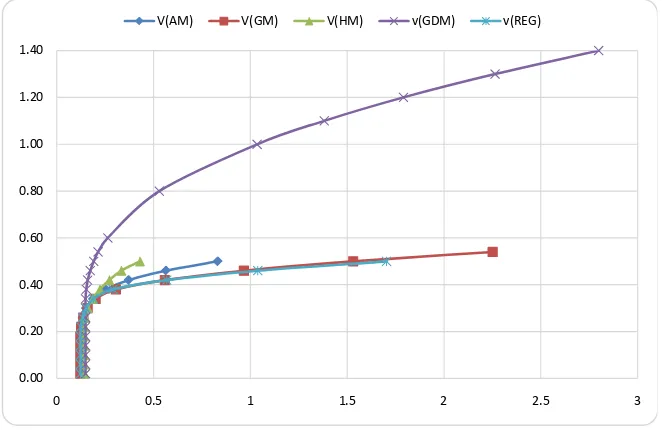
k value. The four efficient frontiers are shown in Figure 1.

For a given risk free rate RF, the greatest tangent angle attainable between

the ray from RF and the efficient frontier curve can be calculated from

Equa-tion (5). By verifying RF we find the optimal tangent angle via LINGO and

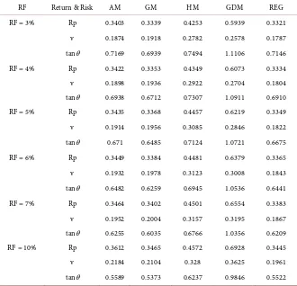
report the portfolio returns portfolio risk (υ) and tangent angles (tan θ) in Table 4. An inspection of Table 4 reveals that Sharpe’s solutions with GDM dominates that with HM for RF = 3%, 4%, 5% and 6% because return under GDM are

greater but risks smaller than that under HM. For RF =7% and 10%, returns and risks are both greater under GDM in comparison to HM. Hence we calcu-late Sharpe’s index orits tan

θ

A comparison between AM and GM indicates that risk-return combinations using AM dominate that using GM: higher return with less risk from RF =3% through 7%. At RF =10%, both the portfolio return and risk are greater using AM: 0.3612 > 0.3465 and 0.2184 > 0.2104. As a consequence, we compare tan θ

Figure 1. Efficient frontier curves using five different means.

0.00 0.20 0.40 0.60 0.80 1.00 1.20 1.40

0 0.5 1 1.5 2 2.5 3

DOI: 10.4236/tel.2018.83025 365 Theoretical Economics Letters

Table 4. Angle maximization solutions using five means.

RF Return & Risk AM GM HM GDM REG

RF = 3% Rp 0.3403 0.3339 0.4253 0.5939 0.3321

v 0.1874 0.1918 0.2782 0.2578 0.1787 tanθ 0.7169 0.6939 0.7494 1.1106 0.7146

RF = 4% Rp 0.3422 0.3353 0.4349 0.6073 0.3334

v 0.1898 0.1936 0.2922 0.2704 0.1804 tanθ 0.6938 0.6712 0.7307 1.0911 0.6910

RF = 5% Rp 0.3435 0.3368 0.4457 0.6219 0.3349

v 0.1914 0.1956 0.3085 0.2846 0.1822 tanθ 0.671 0.6485 0.7124 1.0721 0.6675

RF = 6% Rp 0.3449 0.3384 0.4481 0.6379 0.3365

v 0.1932 0.1978 0.3123 0.3008 0.1843 tanθ 0.6482 0.6259 0.6945 1.0536 0.6441

RF = 7% Rp 0.3464 0.3402 0.4501 0.6554 0.3383

v 0.1952 0.2004 0.3157 0.3195 0.1867 tanθ 0.6255 0.6035 0.6766 1.0356 0.6209

RF = 10% Rp 0.3612 0.3465 0.4572 0.6928 0.3445

v 0.2184 0.2104 0.328 0.3625 0.1961

tanθ 0.5589 0.5373 0.6237 0.9846 0.5522

i i

Rp=

∑

( )

tanθ=

∑

and find that under AM is greater 0.5589 > 0.5373.

5. Concluding Remarks

In this paper, we calculate four different kinds of means—AM, GM, HM, and GDM—to investigate the risk-return contour using Markowitz risk minimiza-tion and Sharpe’s angle-maximizaminimiza-tion models. For a given k value (target portfo-lio return), the rank order of risk or variance-covariance (υ) can change. In the vertical segment of an efficient frontier curve, we observed v(GDM) > v(HM) > v(GM) > v(AM). At higher k values, the rank changes to v (GDM) > v(HM) > v(AM) > v(GM). That is to say, ranking a portfolio using different kinds of means may well give different rankings depending on what k value one is eva-luating.

DOI: 10.4236/tel.2018.83025 366 Theoretical Economics Letters and AM over HM and GM respectively for greater angle translates into high portfolio return (net of Rf) per risk. Care must be exercised though; the results from this paper are limited to the stocks that we take in the sample. However, comparative evaluations are needed for a comprehensive analysis on a portfolio performance. In sum, GM is less sensitive to outliers and hence is more suitable for conservative strategy. GDM is determined by the size of its range and tends to offer an optimistic forecast on mean return especially when there exist a few unusually large positive returns. Finally, HM is not appropriate if some of the returns (%) are small and negative. In that case, HM ought to be removed from the analysis.

References

[1] Markowitz, H. (1952) Portfolio Selection. Journal of Finance, 7, 77-91.

[2] Markowitz, H. (1952) The Optimization of a Quadratic Function Subject to Linear Constraints. Naval Research Logistics Quarterly, 3, 111-133.

https://doi.org/10.1002/nav.3800030110

[3] Markowitz, H. (1959) Portfolio Selection: Efficient Diversification of Investment. John Wiley & Sons, Inc., New York.

[4] Sharpe, W.F. (1964) Capital Asset Prices: A Theory of Market Equilibrium under Condition of Risk. Journal of Finance, 19, 425-442.

[5] Goto, S. and Xu, Y. (2015) Improving Mean Variance Optimization through Sparse Hedging Restrictions. Journal of Financial & Quantitative Analysis, 50, 1415-1441.

https://doi.org/10.1017/S0022109015000526

[6] Yang, C.W., Hung, K. and Yang, F.A. (2002) A Note on the Markowitz Risk Mini-mization and the Sharpe Angle MaxiMini-mization Models. In: Lee, C.F., Ed., Advances in Investment Analysis and Portfolio Management, Vol. 9, Elsevier Science, Amster- dam.

[7] Gil-Bazo, J. (2006) Investment Horizon Effects. Journal of Business Finance & Ac-counting, 33, 179-202. https://doi.org/10.1111/j.1468-5957.2006.01098.x

[8] Best, M.J. and Grauer, R.R. (1991) On the Sensitivity of Mean-Variance-Efficient Portfolios to Changes in Asset Means: Some Analytical and Computational Results. The Review of Financial Studies, 4, 315-342. https://doi.org/10.1093/rfs/4.2.315

[9] LINGO 8.0 Linear and Nonlinear Optimizer. LINGO System Inc., Chicago, IL, 2003.

[10] Elton, E.J., Gruber, M.J., Brown, S.J. and Goetzmann (2007) Modern Portfolio Theory and Investment Analysis. 7th _{Edition, John Wiley and Sons, Inc., Hoboken,}