Convective instabilities in binary fluids

warwick.ac.uk/lib-publications

A Thesis Submitted for the Degree of PhD at the University of Warwick

Permanent WRAP URL:

http://wrap.warwick.ac.uk/102295

Copyright and reuse:

This thesis is made available online and is protected by original copyright.

Please scroll down to view the document itself.

Please refer to the repository record for this item for information to help you to cite it.

Our policy information is available from the repository home page.

T H E B R I T I S H L I B R A R Y D O C U M E N T SUPPLY C EN TR E

TITLE

_{Convective instabilities in binary fluids}

A tten tio n is drawn to the fact that the copyright of

this thesis rests with its author.

T h is copy of the thesis has been supplied on condition

that anyone w h o consults it is understood to recognise

that its copyright rests with its author and that no

information derived from it may be published without

the author's p rior w ritten consent.

A U TH O R

David Holton

IN STITU TIO N

and DATE

u/uu/citvy

ih

»

s

I

M l" I 21 I 31 Boston Spa, W e t I W est Yorkshire — I United Kingdom

T H E B R I T IS H L I B R A R Y

D O C U M E N T S UPPLY C E N T R E

Boston Spa, W etherby

20

R E D U C T I O N X

C o n te n ts

A C K N O W L E G E M E N T S “

A B S T R A C T 1

C H A P T E R 1 - The physics o f double diffusive convection 2

1.1 A b s t r a c t ... 2

1.2 M echanism for in s t a b i lit y ... 2

1.3 Equations o f m o t i o n ... 4

1.3.1 Navier-Stokes e q u a t i o n s ... 4

1.3.2 In c o m p r e s s ib ility ... 6

1.3.3 Conservation o f e n e r g y ... 6

1.3.4 Conservation o f species ... 7

1.3.5 E quation o f s t a t e ... 7

1.3.6 Phenom enological effects-the Soret a n d D u fou r effects 8 1.3.7 E quations o f m otion : collated ... 10

1.4 Boundary c o n d it i o n s ... 12

1.5 S y m m e tr ie s ... 13

1.6 C o d im e n s i o n -2 ... 14

1.7 Therm ohaline, therm osolutal, doubly and m ultiply diffusive c o n v e c tio n ... 14

1.8 Nusselt n u m b e r ... 15

C H A P T E R 2 - Dynamical systems theory jy 2.1 A b s t r a c t ... n 2 .2 Dynam ical s y s te m s ... ig 2.3 An o v e r v ie w ... 19

2 .4 Bifurcation t h e o r y ... 21

2.5 Centre m anifold theory ... 23

2.6 E xam ple-the Lorenz m o d e l ... 26

2.7 Reductive perturbation theory ... 28

2.8 Hopf b i f u r c a t i o n ... 29

2.9 A pplications o f Lie g r o u p s ... 30

2.11 Extensions to the ñnne - dim ensional centre m anifold theory C H A P T E R 3 - T r i c r i t ic a l b ifu r c a t io n

3.1 Introduction to the tricritic&i bifurcation - ... - 32

3.2 The m echanical a n a l o g u e ... 33

3.3 Linear t h e o r y ... 34

3.4 Critical Rayleigh number with idealised b o u n d r i e s ... 35

3.5 Linear theory w ith real b o u n d a r ie s ... 36

3.6 The < h e ir a r c h y ... 36

3 ' 0 ( « ) ... 39

3.8 O ^ ) ... 40

3.9 0 (t> ) ... 41

3.10 0 ( « 4) ... 44

3.11 The am plitude e q u a t i o n ... 45

3.12 Calculation o f the Nusselt n u m b e r ... 46

3.13 Experimental e v i d e n c e ... 46

3.14 Slow spatial m o d u l a t i o n ... 47

3.15 Imperfect sym m etry ... 49

3.16 Steinberg a p p r o a c h ... 49

C H A P T E R 4 - T h e d e g e n e r a t e H o p f b ifu r c a tio n 4.1 H opf b i f u r c a t i o n ... 50

4.2 Linear t h e o r y ... 53

4.4 OÍ«3) 56 4.5 0 (« * ) ... 5 7 4.6 Cailculation o f the left eigenvector o f Lt ... 58

4.7 Am plitude equation at third o r d e r ... 59

4.8 Solution to third o r d e r ... 61

4.9 0 ( « 4) ... 62

4.10 Predictions versus r e a lity ... 65

4.11 Equivariant bifurcation theory for the degenerate a n d non­ degenerate H opf b ifu r c a t io n ... 68

4.12 * ( 3 ) - 0 ? ... 71

C h a p t e r 5 - S c h e m e s o f G a le rk in tr u n c a tio n s 73 5.1 The m ethod o f G a le r k in ... 73

5.2.1 How do we t r u n c a t e ? ... 77

5.3 The truncation hierarchy ... 79

5.4 Galerkin truncation o f Galerkin a n d Saltzm an... 80

_5.5 Aside: an alternative a p p r o a c h ... 82

5.6 The stationary b ifu r c a tio n ... 84

5.6.1 Five m ode m o d e l ... 84

5.6.2 5 -m ode minimal r e p r e s e n ta t io n ... 84

5.6.3 8 -m ode m o d e l ... 86

5.6.4 14-mode representation ... 88

5.7 The extended Galerkin m o d e l ... 89

5.8 Invariant su b sp a ces... 92

5.9 Linear t h e o r y ... 93

5.9.1 Pitchfork b ifu r c a t io n ... 93

5.9.2 H opf b i f u r c a t i o n ... 94

5.9.3 Tricritical bifurcation ... 95

5.9.4 Broken tncritical s t a t e ... 95

5.10 Basic properties o f the tru n cation s c h e m e ... 96

5.11 Far from c r i t i c a l i t y ... 97

C h a p t e r 8 - C o n c lu s io n s 99 C o n c lu s io n s ... 99

Appendix 1 101

Appendix 2 106

Appendix 3 1Q7

Appendix 4-, 5

110,111

Figure 1.

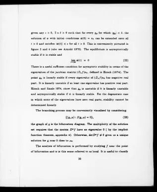
A single fluid in a cylindrical dish heated from b elow . Flow patterns at several values o f e, taken from V. Steinberg et a i.(1 98 5 ). T h e values o f e are (a ) 0.29; (b ) 0.18; (c ) 0.13; (d ) 0.08; (e ) 0.02; ( f ) -0.06. Patterns a and b represent concentric flow. For the rest, excep t ( f ) the concentric flow is unstable, but the evolution o f the pattern is slow and images do not represent a steady state. This figure dem onstrates the phenom ena o f critical slowing dow n near the point o f bifurcation.

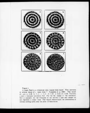
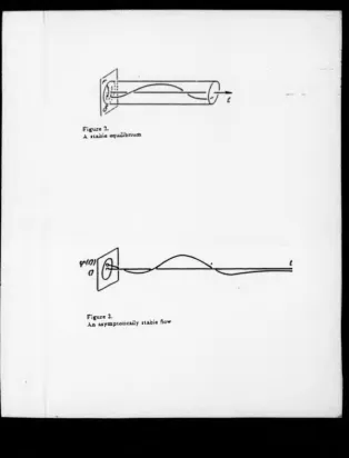
Figure 2. A stable equilibrium Figure 3.

A n asym ptotically stable flow Figure 4.

T h e roll configuration in a layer o f fluid. The various symmetries are shown.

Figure 5.

T h e pitchfork and broken pitchfork bifurcations. Figure 6.

Benjam in's apparatus for dem onstrating the buckling o f a viscoelastic arch o f wire (taken from D .D . Joseph (1983))

Figure 7.

T h e tricritical bifurcation, the arrows indicate the hysteretic phenom ena Figure 8.

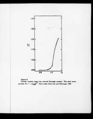
Nusselt num ber verses the reduced Rayleigh n um ber. The solid curve satisfies N u — 1 = (¡35-f*. D ata taken from G ao and Bellringer 1986.

Figure 9.

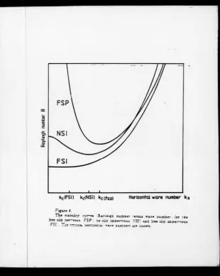
T h e stability curves (R ayleigh number versus w ave num ber) for the free slip pervious (F S P ), no slip im pervious (NSI) a n d free slip im pervious (F S I). The critical horizontal wave numbers are shown.

Figure 10.

X versus tim e at onset o f convection for the eight m od e problem . It shows the characteristic predp itious relaxation to the oscillatory state. This state becom es unstable to a fixed point.

Figure 11.

Figure 12.

A'! versus Y\ for the five m ode m odel before and after the period d o u ­ bling bifurcation.

Figure 13.

Schem atic representation o f the period doubling cascade to the h etero­ clinic explosion (M oore et al 1983).

Figure 14.

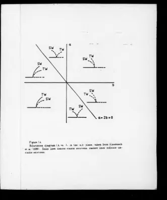
Bifurcation diagram (A vs. A) in the (a ,b ) plane, taken from K n o b lo ch et al (1986). Solid lines den ote stable solutions, dashed lines in dicate un­ stable solutions.

Figure 15.

M e m o r a n d u m

A c k n o w le d g e m e n ts

The author wishes to express his thanks to all who made the com pilation o f this thesis possible. I would especially like t o mention Dr. George Rowlands for his supervision and friendship throughout.

I also like to thank D r J.K . B hattacharjee and Dr. P Lucas at M anch­ ester University for useful correspondence a n d suggestions throughout the study o f the H op f bifurcation.

A b s t r a c t

The subject o f two-dimensional convection in a binary fluid is treated by analytical methods and through Galerkin models. The analysis will focus on describing the dynamics o f convection at onset of convection. Two independent dynamical parameters are present- one more degree o f freedom than single fluid convection.

We shall derive normal forms for the tricritical bifurcation - de­ scribing the transition between a forward and backward pitchfork bi­ furcation o f a two - dimensional array of rolls in a convecting bulk binary fluid mixture. A multiple time perturbation scheme is con­ structed to fifth order to describe this motion. The coefficients of the equation are determined as a function o f the Lewis number ( the ratio of the mass to thermal diffusivity ). The degenerate Hopf bifurca­ tion is also investigated using a similar perturbative scheme; with a prediction o f the coefficients involved.

A model system, using a ’minimal representation^ Veronis 1968) gives rise to a Galerkin truncated scheme (a set of 14 ordinary differ­ ential equations). It is claimed that the dynamical character of both the tricritical and degenerate Hopf bifurcation are included in the zo­ ology o f the bifurcation behaviour at onset o f convection. These and other dynamical aspects o f the equations are investigated.

In an attempt to improve upon free slip pervious boundaries a projection o f the equations is made onto a more appropriate subspace. A comparison with experimental evidence is given.

C h a p te r 1 - T h e P h y s ic s o f D o u b le D iffu ­

sive C o n v e c tio n

1.1

A b stra ct

This chapter contains the basic physics required to describe the convective process in a binary fluid. T h e two fluids will be taken to be com pletely miscible. The basic equations o f m otion for convection in binary fluids are presented.

1.2

M ech an ism for in stab ility

trying to equilibrate local com position. The critical observation is that when the stressed fluid undergoes a convective cycle the particle m ay end up with a m arkedly different com position. Hence, it may over o r under shoot its original position and undergo oscillatory behaviour. A t o n s e t o f convection (from the conductive state) we m ay observe oscillatory be­ haviour in dou ble diffusive systems (in contrast to a single fluid) due to the fluid m otion being unable settle in a steady state configuration due to the element o f fluid loosing bgGVancy through two u n e q u a l processes: ther­ m al diffusion and mass diffusion. The mass diffusion may act to enhance or retard convection.

T h e subsequent spatial pattern we observe is highly dependent upon m any factors. Geom etry o f the cell in which the fluid is contain ed, its size (asp ect ra tio) and shape all play an im portant role in determ ining the dynam ical flavour o f the flow. T h e geom etry o f the container, will effect the sym m etry, if any, o f the problem . A number o f flow patterns shadow- graphically visualised for a fluid heated from b elow in a cylindrical dish, ob tained from experiment o f Steinberg et al 1985, are shown in fig. 1, to show the dynam ical variety.

T o render analysis tractable, an infinite b o x or periodic b ou n d a ry con­ ditions are often used to m odel experiment. In a finite b o x , for instance, any translational invariance due to the im posed periodicity will b e lost. In the analysis that appears in this thesis the simplest possible configuration.

that o f a regular array o f roll solutions shown in fig. 4 will be considered, realisable in rectangular b oxes in which the rolls align themselves parallel to the shorter side. O ther configurations, such as hexagonal or Bénard type cells will not be treated.

T o summarise: the underlying mechanism o f oscillation is the discrep­ ancy between the relaxation times for thermal and concentration fluctua­ tions. This in turn gives rise to extra dynam ical behaviour at the onset o f convection.

1.3

E qu ation s o f m o tio n

1.3.1 The Navier-Stokes equations

W e shall consider a horizontally infinite layer o f binary fluid infinite in the lateral direction and o f constant thickness d . It will start with linear gradients o f tem perature and concentration in equilibrium; see equations (11) and (1 2 ). This we shall call this the conductive regime. A particle o f hom ogeneous fluid, binary o r otherwise, will ob ey the following equation o f Navier-Stokes:

‘¡2 - + Ç . V V

V P + j S - + v V ' V ,

1

(ft Pm pm

where V is the velocity, p ,p m »the density and mean density respectively. The other variables are the hydrostatic pressure P , gravitational constant

g, and u kinematic viscosity. We have used the usual Boussinesq approx­

imation ( Chandrasekar 1 981) in which all o f the physical parameters may

be regarded as constants except the density when it multiplies the bulk force term . This approximation seems to b e in keeping with m ost realistic, controlled experiments. Equation (1 ) is art expression o f the conservation of m om entum . The only ambiguity, as p oin ted out in the text b ook on fluid m echanics by Landau and Lifschitz [1959] is in the definition o f velocity for a bin a ry fluid, i.e. which fluid’s velocity axe we measuring? However, after a m om en t’s thought this ambiguity m ay b e overcom e by sim ply defining the velocity as the m om entum density per unit volume divided by density. The left-hand side o f eq u ation (l) m ay b e m ore concisely written in terms o f the usual Eulerian description o f an ’a dvective’ or total derivative:

D V

D t — + ? . v ? , (2)

as the velocity is a function o f space and tim e. The velocity is a vector quantity V = (u,v,w ). W e will eventually assume that the basic state we are interested in is a roll solution (schem atically represented in fig 4 ), in which we may regard v = 0 .

A three-dimensional description m ay b e developed through either de­ veloping the third dim ension as a spatial perturbation on the basic roll solution (Segal 1969) or through im p osing a physically realisable three di­ m ensional pattern, e.g. a hexagonal pattern (Hohenberg P.C . and Swift J.B . 1987).

1 .3 .2 I n c o m p r e s s i b il it y

We assume the fluid to be incompressible. W e also assume the fluids are non-reacting and hence, assume there are no chemical processes going on. Consequently, we obtain the result:

which makes our vector field solenoidal. At this point we m a y combine equations (1 ) and (3 ). T his results in expressing the velocity, in the two dim ensional case, in term s o f a stream function i>. The velocities in the

1.3.3 Conservation o f Energy

An equation for the tem perature m ay b e derived using conservation o f energy. W e use in its derivation various therm odynam ic relations, details o f which are given in appen dix 1. The equation for the tem perature T takes the particularly simple form :

V .V = 0,

₍₃₎

horizontal and vertical directions can then be written as = uj and ■

(4 )

1 .3 .4 C o n s e r v a t i o n o f s p e c ie s

For a binary fluid we define c to be the concentration o f the lighter fluid. The corresponding equation for c is;

D c 1 _ .

D t “

(5)

where j is the mass flux o f the lighter com p onent. This expression may be generalised to include internal generation o f heat. We will however restrict ourselves to realistic experim ental circum stances in which we may neglect these generalisations.

1.3.5 The equation o f state

One last expression we require to fully describe the equations for the bi- nary fluid is for the density. W e adopt the simplest non-trivial equation o f state for the density t o take into consideration its functional dependence on the tem perature and concentration (i.e. the lowest order nontrivial Taylor expansion):

? = ^ [ l - a ( r - r . ) - / 9 ( c - e o ) ]

(6)

where a = ( ! ? ) _ end 0 = —

J (S f)r

b ou n d a ry conditions in the lateral direction are taken as period ic. Period­ icity is specified purely for simplicity. Periodic boundary con d ition s may be th ou gh t to be valid for an infinite or sufficiently large b ox. T h is intuitive in terpretation o f the infinite box can b e misleading. The horizontal plates th a t b ou n d the fluid should be take t o be rigid and allow n o mass flux across the boundary. Rigidity ensures that the normal co m p on en t o f the velocity field at the top and b ottom boundaries is zero. T h ese conditions will b e relaxed to make the analysis tractable. These a pproxim ations will b e addressed after the fluxes i and q are given.

1 .3 .6 P h e n o m e n o lo g i c a l e ffe c ts - t h e S o r e t a n d D u f o u r e ffects

T h e m ass diffusion flux i, and the heat diffusion flux q, are due to the presence o f temperature and concentration variations in th e fluid. One m a y naively guess that the heat flux is linearly related to the gradient o f th e tem perature; this m ay be more familiar as a statement o f Fourier’s law in the conduction o f heat down, say a b a r o f metal. Analogously, the mass flu x m a y be considered proportional to the gradient o f the m ass distribution (th e gradient o f concentration). However, this picture is largely incomplete a n d inaccurate. Generally, each flux will depend on a linear com bination o f gradients o f tem perature and concentration. Using O nsa ger’ s (Onsager 1932) reciprocal relations this can be concisely stated as:

. » - « ( B V c - r - y i r r ) , (8 )

where.« = k r D . kj- is the thermal diffusion ratio. D the mass diffusion co­ efficient, n the difference in the chem ical potentials o f the two com ponents. k the thermal con d u ctivity and p the density o f the m ixture ( see Landau and Lifshitz 1958, D eG rout and M azur 1970 and Lee Lucas and Tyler 1983 )•

If pressure variations were im portant then the gradient o f pressure would appear in equation (8 ). T h e inclusion o f the terms proportional to V T in equation (8 ) was first recognised to b e im portant b y S cret' «. Its inclusion is now com m on ly refered to as the Soret effect. T h e converse effect-a flow o f heat due to the presence o f a concentration gradient is normally refered t o as the Dufour effect. The theoretical origins o f these effects are discussed in great detail in chapter X I in D eG root and Mazur (1962). Experim entally the Soret effect is observed to b e at least an order of magnitude larger tha n the Dufour effect (Lucas et al 1983). Consequently, the Dufour effect is largely neglected. Although they are related b y Onsager relations the gradient o f tem perature V T is much bigger than V c , suitably non-dim ensionalised.

In cryogenic H e 3 — H e* norm al fluid mixtures the D ufour effect can be significant, especially near the therm odynam ic tricritical point (Lucas et al 1985). T h e divergence o f several physical quantities near to the ther­ m odynam ic tricritical point may be utilised in exploring large regions of

param eter space. In the analysis th a t follows we shall include the Dufour effect until its inclusion becom es unm anageable. We will discover that the expression for the general binary fluid can b e simplified t o an uncoupled thermohaline type by a linear change o f coordinates, this was first pointed ou t by K nobloch (1980).

1.3.7 Equations o f motion : collated

I f we substitute equations (7 ) a nd (8 ) in to equations (4) and (5 ) we obtain:

(V.7 + ^ ) t . i V ' c + ^ n

(9)

(V .v + ¿ ) r = (i>T + X B )V ’ r + _{l7t K} (10)

t

where A = (| ^ )r /TCP is a m easure o f the Dufour effect.k r, the ther­ m al diffusion ratio is found to sm all experimentally. T h e D ufour effect is o f O(fcy) and the Soret effect is O (fc r ), consequently the D ufour effect is usually neglected. A ll o f the relevant experimental work on binary fluid m ixtures has been perform ed in th e absence o f an external field causing a significant pressure gradient. T h is is precisely why equation (10) lacks a term proportional to V 3P (see L a n d au and Lifshitz 1958). O ne would also expect in general that frictional fo r ce s w ould cause internal heating; this w e also consider to have negligible effect.

T h e analysis will concentrate on perturbations from criticality. T h e sub- critical state being characterised b y a non-convective, linear tem perature

and concentration distribution given by:

(12)

( 1 1 )

W e may collect together equations (1 )-(10 ) and consider the equations o f

In writing dow n equations (13-15) we have ch osen to neglect the Dufour effect, w is now the scaled vertical com ponent o f velocity, Dt — k — k rD

m om entum equation. The steps in its derivation are routine. The operator

j . V x V x , w hich serves to eliminate pressure fr o m th e m om entum equation,

is applied to equation (1 ). Equation (6 ) is used t o give the equation for the tem perature (in rescaled variables the tem perature perturbation is 0 ). T h e Prandtl num ber, a — -¡fa, the Lewis number L = = ¡^ , the Rayleigh number R = , V is the separation ratio = A j is the Lapladan, in its two dim ensional representation : A = ^ and A ] = ^ y.

m otion from the motionless quiesent state. W e scale time with velocity with tem perature with and concentration with A natural grouping o f param eters occurs for the tw o-dim ensional problem :

A ( - ^ - ) = <rA*t» + ctA 2(0 + e ), (13)

(14)

— = L A c — ij>LA0 + ivRw. (15)

and 0 is chosen interchangeably with T . Equation (1 3 ) is obtained from the

1.4

B o u n d a ry con d ition s

It is clear from the subsequent sections that the dynamics o f b in a ry fluids are govern ed by a set o f p .d .e .’s involving the dependent variables 9. c and w in a fluid domain D with coordinates i * . z). W e must sp ecify what happens at the boundary d D . T h e boundary o f the fluid is usually taken to be rigid, suffering no deform ation; so the normal com ponent o f the velocity field is taken to be zero. T h e concentration flux, must also vanish o n d D , indicating n o bodily movement o f fluid across the boundary-a c o n d itio n o f im perm eability. Impermeability and rigidity can be stated concisely as:

6 = i = v = D w = 0, z = 0 ,1 (1 6 )

The linearised version o f the equations can be solved for the stationary p rob ­ lem in closed form in terms o f hyperbolic functions (see G utkow itz-K rusin (1979) a n d in its corrected form by Lucas et al (1983)). T h e linearised form o f equations (13)-(15) have been studied extensively by S chechter et al 1974. T h e form o f the linear solution is straightforward, though la b oriou s to m a nipulate. Weakly nonlinear theory is rendered hopelessly tir e so m e if the im p erviou s rigid boundaries are used as a basis for the con s tru ction o f an a m p litu d e equation.

T o circum vent this problem we adopt free slip pervious b o u n d a ry con­ ditions:

9 = c = w = D 2w = 0, z - 0 ,1 . (1 7 )

T h e ’rigid’ condition D w = 0 c o m e s from the fact that u and v. the com p o­ nents o f the velocity perpendicular to w are identically zero on the b ou n d­ ary for all x and y. C onsequently, using the incompressibility condition V .V = 0, §jf = §J * 0 (as u a n d v are constants on the bounda ry), and hence D w = 0. For the ’slip’ con d ition D 2w = 0, we require the stress ten­ sor to vanish giving fi (|* + = 0. Differentiating the incompressibility condition with respect to z gives th e required result D 2w — 0.

The conditions in the lateral (x -d irection ) will be taken to be periodic.

1.5

S ym m etries

In a laterally infinite system , laterally periodic boundary conditions may be chosen. In a finite b o x , the system would no longer be translationally invariant.

W e shall asstime that the flow has the form o f a two-dimensional array o f rolls ( spatially periodic o f p e r io d j^ ). An additional requirement, which is supported by the equations them selves, is a refiectional sym m etry in any vertical plane. T h e totality o f these symmetries mean that the system possesses 0 ( 2 ) symmetry, the rota tion s and reflections o f the circle. It is the presence o f this sym m etry th a t determines the structure o f the normal form for a local bifurcation.

1.6

C o d im e n s io n 2

T h e reduced system as given by equations (1 3 )-(1 5 ) contains tw o experi­ mentally tunable parameters: the Rayleigh number R , and the separation ratio v . T h e tw o parameters are independently adjustable. The Rayleigh number is the nondimensionalised version o f the tem perature difference be­ tween the two bounding surfaces. The separation ra tio is a nondimension­ alised version o f the concentration gradient. The separation ratio contains the cross coupling between the tem perature and concentration gradients, the thermal expansion coefficient, and the derivative o f the density with respect to concentration.

The separation ratio can be m ade to change sign, for instance, by chang­ ing the relative com position o f the mixture.

A dynam ical system containing two independently adjustable parame­ ters is usually refered to as a two parameter family. T hen it is interesting to look for bifurcation phenom ena o f codimension 1 a nd 2, since they occur stably in two parameter families. C hapter 2 will clarify its usage.

1.7

T h erm oh a lin e, th erm osolu ta l, d o u b ly and m ulti­

p ly diffusive c o n v e c tio n

All o f the above terms are essentially manifestations o f the same phenom ­ ena. Therm ohaline and thermosolutal convection refer to solutions o f salt and solute respectively, in which case the Soret and Dtifour effects are ab­

sent. D ou bly and multiply diffusive convection are generalisations as they are ph enom ena that involve two and many diffusive processes respectively.

T o be m ore precise, dou bly diffusive convection is generally referred to as con vection in a fluid layer with a stabilising concentration gradient.

E xam ples o f experiments are quite diverse, the fluids in question vary from cryogenic 3 H e — 4H e normal fluid mixtures to alcohol-water systems. The excellent thermal properties o f 3H e — 4H e (Ahlers 1978) give this pair many advantages over salt-water and ethanol-water system s. T h e notice­ able draw back in the use o f low tem perature mixtures is that flow visuali­ sation b ecom es impossible.

1.8

N u sselt nu m ber

As it is im practical to visualise the flow in som e experim ents it is im ­ portant to have an alternative way o f confirming predictions from theory. The heat transported across the fluid layer is one quantity that can be measured and compared with the theory. The appropriate quantity is a □on-dim ensionalised version o f the heat flux called the Nusselt number and is given b y:

see Busse (1 9 79 ) for details.

T h e disadvantage with this is that it averages out spatial in h om o­ geneities a n d hence we receive incom plete information if we wish to in­

(18)

vestigate the spatial dynam ics o f the flow.

Physically, the Nusselt num ber m ay be understood as a ratio o f con d u c­ tivities, that is the heat transfered in a convecting state to heat transferred in a conducting state.

C h a p t e r - 2 D y n a m ic a l sy ste m s th e o r y

2.1

A b s t r a c t

T h e ob je c tiv e o f chapter 2 is to gather relevant mathematical material to answer, at least partially, the questions posed in chapter 1. Selection will be m ade from aspects o f dynam ical systems th eory and reductive perturbation theory.

W e m ust always have in mind: what is th e role of dynam ical systems in hydrodynam ics? This is a difficult a nd rather technical question to answer in general terms. W hen the R ayleigh number is sm all there is a unique correspondence between a given set o f boundary conditions and the subsequent flow; this can be proven rigorously by energy m ethods, see Joseph (1976) for details. W hen the Rayleigh number increases this uniqueness fails, a multiple solution state is now the rule. Bifurcation theory a ttem p ts to provide a substantial m ath em atical basis for this study.

2.2

D y n a m ica l system s

D ynam ical system s theory (D .S .T .) is a d iverse and rapidly evolving branch o f m a th em atics. D .S.T. has been used to d escrib e an apparently vast num­ ber o f phenom ena. This is perhaps why it has so much appeal. It has been used, for exam ple, to classify com m on and universal features in systems as disparate as the Belousov-Zhabotinskii reaction in a stirred flow reactor (Sim oyi R .H . 1982) and the Henon m ap. as the forced sim ple pendulum

(K adanoff L 1985) and the phospholipid m onolayer (Langer J.S. 1985).

2.3

A n ov erview o f dyn am ica l sy stem s

A state o f a physical system is information about the system at a given time, that may be contained in a collection o f variables. Suppose, for the mom ent. that the variables X ( t ) are finite in number X ( t ) = (ATi(t), X 2( t ) , ...,AT„(t)). The space o f states o f AT e U C I f 1 is called the phase or state space. Per­ haps X ( t ) is also dependent upon several parameters n = ...fi^). T h e collection o f such /x?s is the parameter or con trol space. W h en the time evolution o f X ( t ) may be expressed in terms o f X ( t ) and fi , we obtain a system o f ordinary differential equations;

f is appropriately called the v ector field, since at each point ( X ; ft) we assign a vector f ( X ; n ) . A solution o f (19) together with an initial condition at t= 0 , is called a trajectory,

is a dynam ical system. Although, studying the equation governing binary fluids one is not dealing with a dynamical system as described a bove but we (19)

X ( < ) = (20)

The collection o f mappings;

(

21

are dealing with, technically a m ore difficult ob je c t - a semi-flow in infinite dimensions. However, we shall see that much o f the interesting behaviour observed in experiments supports the thesis that we may think in terms o f low-dim ensional systems o f equations (L ib ch ab er 1981). This o f course skims over many o f the technical difficulties in m aking the transition from the infinite-dimensional system to the finite-dimensional.

2.4

B ifu rca tion th e o r y

Given a dynam ical system , defined by (19), we m ay wish to understand how qualitative changes in the flow occu r as we vary the param eter y . The variation o f the parameters correspond, for exam ple, to adjusting the tem ­ perature difference across an experimental cell, o r to increasing the available foodstuffs for a species in a population experim ent ( May 1976). T h e "b a ­ sic” state for the convection problem would b e the conductive solution in which the fluid is quiesent. In population dynam ics the basic state may correspond to the population remaining constant in time. A s we change parameters this state m ay lose stability.

W hen a loss o f stability o f the basic state is replaced by a branched or multiple state, resulting in a qualitative change in the flow, we shall call this a bifurcation. In the context o f the exam ples given the new state may be in the form o f an oscillating or time periodic state.

We m ust first address the problem o f what d o we mean by stability? W e take the Lyapunov view o f the flow: An equilibrium £. = 0 is stable if

given any e > 0, 3 a 6 > 0 such that for every Za for which < 6. the

solution o f v> with initial conditions 0 (0 ) = x0 can be extended o n to all

t > 0 and satisfies j0(f)| < 4 for all t > 0. This is conveniently pictured in

figure 3 and 4 (also see A rnold 1978). T h e equilibrium is asym ptotically stable if it is stable and

hm 0 ( f ) « 0 (22)

T h ere is a useful sufficient cond ition for a sym ptotic stability in term s o f the eigenvalues o f the jacobian m atrix ( D x f ) x 0, defined in Hirsch (1 9 74 ). The p oin t Za is linearly stable if every eigenvalue o f ( D af ) x0 has negative real pa rt. It is linearly unstable if at least one eigenvalue has positive real part. Hirsch and Smale 1974, show that Zo is unstable if it is linearly unstable and asym ptotically stable if it is linearly stable. For the degenerate case in which some o f the eigenvalues have zero real parts, stability ca n n ot be determ ined linearly.

T h e branching process m a y b e conveniently visualised by considering:

< ( l . « ) : / ( « . * 0 - 0 } , (23)

the graph o f £ is the bifurcation diagram . The multiplicity o f the solution set requires that the m atrix D Mf have an eigenvalue 0 ( b y the im plicit fu n ction theorem , appendix 4 ). Otherwise, d e t D * f # 0 gives us a unique solution for £ near 0 close t o

(¿o-T h e analysis o f bifurcation is perform ed by studying / near the point o f b ifurcation and is in this sense referred to as local. It is useful to classify

bifurcations and this m ay be most effectively done by classifying according to their codim ension class. Consistent with Guckenheimer and Holmes 1983 we will use cod im en sion to mean, in this context, the smallest number of parameters which contains the bifurcation in a persistent way. An unfolding o f a bifurcation is a fam ily which contains the bifurcation in a persistent way. The concept o f unfolding is central to discuss the structural stability o f a bifurcation p rocess. Perhaps an exam ple will demonstrate this: the pitchfork bifurcation,

* = - / * * + ** = M = 0. (24)

Equation (24) has a bifurcation as passes through zero. It is extremely n on-robu st, in the sense that if we perturb it by changing / ( £ , /x) to / ( t , (x, n , ), w here /(t,M »M *) = “ A** + ** + m«i there is a drastic change to the bifur­ ca tion diagram (see fig. 5). It is im portant to realise that the introduction o f unfolding param eters often corresponds in a physical application to the breaking o f som e underlying symmetry. The pitchfork example dem on­ strates how fragile these bifurcations can b e. However this bifurcation is persistent in m any physical applications. Symmetry forces it to be persis­ tent.

2 .5

C entre m a n ifold th e o r y

C entre manifold th eory ( C M T) gives a beautiful geometrical picture o f the flow in phase space (fo r detailed statements o f theorems see Guckenheimer

and H olm es 1983. Carr 1979. and m ore recently Yanderbauwhede A . 1988). H ow ever, because the approach is indirect it is com putationally unwieldy as w e shall hint at by example.

T h e behaviour o f the solutions to equation (19) is determ ined by the sp e ctra l properties o f D f ( 0). In general we may sub-divide the spectrum o f D f ( 0 ), call it a , in to three distinct pa rts, namely the stable spectrum a , = {A«a|R(A) < 0 } , the unstable sp ectru m a „ * {A«a|J?(A) > 0 }, and the cen tre spectrum a e w {A «a fR (A ) = 0 } . This gives rise to a natural sp littin g o f phase space R* into invariant subspaces:

RT * X . © X u © X t . (25) N o n ze ro solutions in the stable subspace X t decay exponentially, while th ose in the unstable subspace X v blow up exponentially. All bounded solu tion s belong to the centre subspace. T h e Hart m an-G robm an theorem (G uckenheim er and Holm es 1983) states th a t locally, near £ — 0, the flow o f the linearised system a nd equation (1 9 ) are the same via a hom eom orphism (p r o v id e d a non-resonance condition is satisfied ), when the centre subspace is e m p ty : in otherwords the singular p o in t £ = 0 is h yperbolic. For non­ zero hyperbolic points nonlinear term s in / ( £ ) will be im portant. Centre m a n ifo ld theory serves to prove the existen ce o f invaritfit manifolds within w h ich the trajectories reside.

bounded solutions, su ch u periodic solutions. T h e centre m anifold contains all such solutions s o it seems a ppropriate to study the flow on such an ob ject.

2.6

E x a m p le - th e L orenz m od el

Recall the Lorenz eq u ation s (Lorenz 1963) represent a cou p led set o f three quadratic differential equations representing three m odes ( on e for the ve­ locity and two for th e temperature) o f the Oberbeck- B oussinesq equation for fluid convection in a two dim ensional layer heated fr o m below. T h e equations are usually written:

X » * { Y - X ) (2 6 )

Y = p X - Y - X Z (2 7 )

Z = - 0 Z + X Y < r ,p ,0 > 0, (2 8 ) and contain three param eters a (the P randtl num ber), p ( the Rayleigh num ber) and 0 (th e a spect ratio). T h e three m ode truncation accurately reflects the dom ina nt convective properties o f the fluid for R ayleigh num bers

p 2i 1. T h e technique fo r deriving such a m odel will b e discussed in C hapter

5. The Jacobian derivative at Q is the m atrix:

W hen p — 1, this m a tr ix has eigenvalues 0, — (1 + <r) a nd —3 with eigen­ vectors (1 .1 ,0 ), (<r, —1 .0 ) and (0 .0 ,1 ). Using the eigenvalues as a basis for

By com paring coefficients we find ai = 0 and ¿>j = • Hence the dynamics on the centre manifold h (u ) = ( h\ (u), h2(u )) is given by the am plitude equation:

u = ( — + <T))US + O f« 4). (37)

Equations (1 ) and (2) give an expression fo r th e com plete dynam ics that go to determine the qualitative behaviour o f th e Lorenz equations at p = 1. This static problem gives us very little inform a tion about the dynamics o f the system other than at p * 1. W e w ish to approxim ate the centre m anifold (u,u>) = (h \ (u ,p ), h j(u ,p ) ) for the Lorenz equations when p is close to 1. T o d o this we use the same transform ation as given in equation (30) except keep p as a variable parameter. Carrying out this proceedure yields:

We seek a centre manifold that is a hom ogeneous polynom ial o f the variables o f the centre m anifold, p\ and u. Hence, ch oosin g

■+■ cxp>\ + 0 (3 ), (40)

M « » Pi) = + Ca P\ + 0 (3 ), (41)

by substituiton o f the power series (40) and (41) and com p arin g coefficients we obtain:

(1 t<t)3

Equation (42) describes the dynamics in the centre m a nifold.

2.7

R e d u c tiv e p ertu rb a tion th eory

As an alternative to centre m anifold theory, reductive p ertu rb ation theory or the m ethod o f multiple scales provides a substantial m e th o d o f deriving am plitude equations. The first step in performing red u ctive perturbation theory is, as in the centre m anifold approach, to identify the eigenvalues. We expand around p = 1. For p < 1 we know from H a rtm a n ’s theorem that the zero solution is stable. W e expand in a small pa ra m eter c:

and b y introducing many time scales r0 = t, rx = et, r2 — f* t, w e have to lowest order

X\ to be independent o f tx . T h e eigenvector o f L corresp onding to p\ = 1

(

x,

y,

z)

* « ( x , , y „ z ,) + «*(x,, y,,

zt)

+ ....

also,

p = 1 + epj + €2p i + ..., (44)

where D0 = 5 ^ , D x = e ^ j- ,... For p = 1 the stationary solution requires

u ( x „ y l , z l )r ~ (i.i,o ).

To 0 ( t a),

DoX^ + D xX± = L £

D xX , = L X i +

U . )

( i ) +( 4 ')

(46)

(47)

with adjoint or left eigenvector ( X x,Y x, Z x) = (l,<r, 0). The solvability con ­ dition requires (see Nayfeh and M ook 1973)

- ( D i X , + * D XYX) + <rpi X x = 0. (48)

A sufficient condition for solvability is that X x be independent o f rx and

px = 0. Solving to second ord er requires X3 = X x = Yx, Z j = T o 0 ( « * ) ,

1 0 \ ( 0 \

t » x , -K XxZ, ■ (40)

V o ) \ 0 )

This gives the solvability cond ition found from equation (49) by multiplying b y the a d join t derived from equation (45):

Finally,

= n X , +

BXt » , .

, A p — p\)X\ + &Ti (1 + * ) ” ' r w ~ (1 + < r)0

the required form o f the am plitude equation.

x f .

(50)

(51)

perturbative approach will prove to be m ore efficient in the derivation o f the am plitude equations. Details of the techniques are given in two excel­ lent b ooks. Guckenheimer and Holmes 1983 for the centre manifold theory and Nayfeh and Mook 1973 for the perturbative approach.

2.8

H o p f b ifu rca tion

There are many bifurcations that warrant discussion, perhaps the most im portant we shall encou nter, in the context o f convection in binary fluids is the H opf bifurcation. T h e theorem o f H op f we state is taken from Marsden and McCracken 1975 and is due primarily to Hopf 1932 (also Poincare and Andronov).

It states:

Theorem : Hopf b ifurcation theorem for vector fields

Let X H be a C k(k > 4 ) vector field on R2 such that * 0 for all

H. Let D Xm( 0 ,0 ) have distinct, simple com p lex conjugate eigenvalues A(/x) and A(/s) such that for n = 0, §i(A) = 0. Assume **ffi*^ \»mo > 0. Then there is a C k~* function : ( —« ,« ) — * R such that ( Xi, 0 ,m(-^i)) w on a closed orb it o f period as u ( i radius growing like y/Ji, o f the flow o f X for X\ yt 0 and such that /¿(0 ) = 0.

A H op f bifurcation is observed in the Lorenz system at parameter values

( p ,a ,0 ) = (24.7,10. |) (Sp arrow 1983).

2.9

A p p lic a tio n o f Lie groups

Bifurcations, associated with the qualitative change in fluid flow, provides fertile grou n d for the study o f pattern selection. The presence o f a contin­ uous sym m etry ( a Lie group ), forced through the presence o f internal and boundary constraints, has a remarkable effect on the expected dynamics.

From a mathematical point o f view sym m etry often increases the m ul­ tiplicity o f the eigenspectrum whilst decreasing the com plexity o f the non- linearities allowed (Olver 1982). The H o p f bifurcation in the presence o f sym m etry has been in a state o f vigorous stu d y both from a reductive per­ turbative viewpoint (K n ob loch 1985) and from a more form al approach b y using equivariant bifurcation theory. In the presence o f 0 ( 2 ) sym m e­ try a num ber o f interesting phenomena have been observed. Golubitsky and Stewart 1985 rederive the generalised form o f H opf theorem . A few definitions must be made before the theorem o f H opf can be stated.

Definition: T denotes the group o f sym m etries o f the set o f O .D .E .’s o f equation (1 9 ).

Definition: The symmetries o f a steady state solution form a sub group o f T, j r called the isotropy subgroup o f th a t solution.

Definition: The periodic solution X ( t ) has a spatial sym m etry 7 e T if for every t. y X ( t ) * AT(<).

T h eorem : Let I be an isotropy subgroup o f T such that the fixed point

subspace F ix (E ) is two-dim ensional. Assum e that D f(0 ) is such that

D m ~ { c l

£ ) •

<«>

together with the usual transversality condition on the eigenvalues. Then there is a unique branch o f small amplitude periodic solutions to equation (1 9 ) , o f period near 2ir, whose spatial symmetries are E.

2.10

H o p f w ith sy m m e try

Sym m etry also aids in the simplification o f the nonlinearities that are im­ portant. T h e basis o f the m ethod we shall use, called e q u iv a len t bifurca­ tion theory is best explained by example. Assume for the m om ent that the stream function o f a purely 2-D flow may be represented by a superposition o f left and right travelling waves

iH *» x ; <) * [(v + w )eikm + {V + ET)e~**"]«»n*\s. (53)

T h e condition v = w gives a stationary wave. Here,

v = iuf0v (54)

w = —¿wo to (55) where r and w are the com p lex amplitudes o f the left and right travelling waves. In the presence o f 0 ( 2 ) symmetry - the sym m etry o f the circle under reflections and rotations (occuring naturally in the Binary fluid convection

problem because o f the spatial periodicity o f the rolls) then there are three invariants o f the m otion

=

vv

ww

<Tj =

VW

<Tj =

VW

If we construct the vector field from the above invariants then the vector field will be equivariant under these sym m etry operations (see Chapter 4). A n additional sym m etry that arises in the H opf bifurcation 5 ( 1 ) is the phase shift sym m etry - this being due to the temporal sym m etry due to the periodic nature o f limit cycle ( a time shift o f r , t — * t + r , takes you back to the same place.

2.11

E xten sions to th e finite d im en sional C en tre M an­

ifold th eory

Although the theorem stated in section (2 .7 ) is finite dimensional there are possible generalisations. The assumptions that the eigenvalues o f the linearised problem all have non-positive real parts is not necessary (Carr 1979). The equations also need not be autonom ous.

It has been attem pted in this chapter to give a overview o f dynamical systems. Many, many aspects o f the theory have been om itted. It still remains an open question to what degree it has to play in hydrodynamics. However, the prospects look very promising.

C h a p te r 3 - T r icr itica l b ifu r ca tio n

3.1

In tr o d u ctio n to the tric r itic a l b ifu rca tion

For a vector field f with reflectional sym m etry we say that it has Z2 sym m e­ try. This term inology is used because the two element group Z2 = {» , ¿2} acts on the real line, where i is the identity and R x = — x is the reflection operator. Bifurcations o f this type arise often in physical applications. The effect o f this sym m etry group on a bifurcation in binary fluid convection will be explored. In this context the presence o f Z2 sym m etry im plies the presence o f up-dow n refiectional sym m etry o f the convective rolls.

Z2 makes all the terms in the stationary bifurcation od d . W e m a y expect to use equivariant bifurcation theory to the m odel problem . W e then expect t o express the stationary codim ension 1 problem as an expansion, assuming the vector field / to be sufficiently sm ooth:

^

=

(59)

where /x is a bifurcation parameter. For small amplitude A we m a y expect to b e able to expand f as an equivariant Taylor series , i.e. a Taylor series that is invariant under the sym m etry group. It will be the pu rpose o f the beginning o f this chapter to outline basic results we can e x p e c t, based u p on general considerations from equivariant bifurcation theory. Returning to equation (5 9 ), the expanded version takes on the form:

— = (A — a iA 2 — QjA4,....)A .

32

T o 0 ( A *) the a m plitude equation describes the usual pitchfork (bifurcation) provided a j < 0 see fig(2). In non-generic circumstances, or owing to the presence o f som e physical constraint, in which Qj > 0 the term 0( A l ) is

needed if the bifurcation is to be forward and supercritical. Clearly, if 0 3 ,0 4 , etc. > 0 then we cannot hope to describe the instability in terms o f a small am plitude expansion (in a local sense).

We consider, for the m om ent, equation (3.1) retaining term s up to 0 ( A ‘ ) with the coefficient o f A % normalised. W e expect the stationary bifurcation to differ from the usual pitchfork bifurcation, b y Ahlers (1 9 80 ). This is perhaps m ost easily visualised via the bifurcation diagrams depicted in fig 6, where the solid line denotes a stable branch and the broken line is an unstable branch. This bifurcation has been recently christened the tricriti- cal bifurcation. T h e experimental verification o f this bifurcation has been the subject o f som e controversy in the literature (Ahlers (1 9 86 ), G ao and R ehd berg(1986)). W e will address ourselves to the tricritical bifurcation, in detail, in this chapter.

3.2

T h e m ech an ical analogue

A simple m echanical analogue o f the tricritical bifurcation was given by Benjamin (see Joseph(19 7 7)). Consider an arch o f wire passed through a rigid board, buckling o f the wire is observed as the length o f wire. I is increased see F ig(6 ). This buc)4ng m ay occu r with equal probability to the left or right assuming exact symmetry.

W hen 1 is small, the arch o f wire remains upright, the angle measured from the vertical, 0 = 0 is stable. T h e solution 0 = 0 becom es unstable when the wire reaches a critical length, le, where upon the wire flops to a value 0e. A s the wire is shortened it remains in the sym m etry broken state until a p oin t 1* is reached where the wire flips back to the symmetric upright position. This example shows hysteresis, characteristic o f the tricritical bifurcation.

3.3

L inear th eory

W hen the am plitude o f convection is small enough that the advective terms V .V V , V .V 0 and V .V c can be neglected, equations (1 .5-1.7 ) become lin­ ear. The instability o f the static or conductive layer occu r in the form o f m onotonically (exponentially) growing disturbances. T h e analysis of con­ vection near marginal stability can b e restricted to the time-independent problem (fo r the single fluid); this is generally known classically as the "principle o f exchange o f stabilities” ( Chandrasekar 1954).

The usual stability problem associated with equations (13-15) together with the bou n da ry conditions (1 7 ) is to find the smallest temperature gra­ dient which allows undamped solutions o f the linearised equations. In the free-free (b o th bounding surfaces free slip), pervious perfectly conducting boundary situation a disturbance o f the form

exp( ik .x )s in ( ), (61)

will be a solution at criticality. It becom es unstable for R > Re, where Re is a critical value o f the Rayleigh number.

3.4

C r itic a l R ayleigh n u m b er w ith id ea lised b ou n d ­

aries

The linear operator A associated with the linearisation o f equation( 13-15) o f chapter 1 is;

with Wo = (w o, 6o, **o)» where A = dxx dtt is the tw o dimensional

Laplacian. T h e vector w*o is periodic in b oth x and z, that is, uTo oc

xvo sin k zz cos kxx . This in turn gives the matrix equation Au70 = L«50 = 0.

The critical Rayleigh number is determined from the cond ition for non­ trivial solvability, det(L ) = 0. T his gives when the period ic ansatz (61) is substituted in to equation (62):

We may represent this stability relation graphically. By fixing A and L the critical wave number which will b ecom e unstable is fc. = ^ , (found by calculating j p f ) , kx = n and gives,

A * ( 1 + * ) $ . . - r p d „ R A L A A

0 A 1 (1 + A ) A

(6 2 )

« * ( ( 1 + * ) ( ! + A ) + { ) '

(6 3 )

R,

4 « l + V - ) ( l - A ) + £ ) ' (6 4 )

3.5

Linear th e o r y w ith realistic bou ndaries

In experim ents, the above b oundary conditions are unrealistic. T h e b ou n d ­ aries are rigid and im pervious. However, away from the boundary layer for the rigid case we could possibly expect a situation that simulates the free- slip case. The linear theory for the more realistic boundaries have been treated by Hurle and Jakeman (1970), and subsequently by others, num eri­ cally. The stability diagram for the rigid im pervious case has the sam e fea­ tures as for the free, pervious case, except that the critical Rayleigh num ber is a fa ctor o f 2.1 times smaller than in the rigid case. Pseudo- variational techniques (Schecter et al 1970) have been used to circumvent unnecessary calculation in the H op f b ifurcation observed in linear theory. Linear theory utilising experimentally realistic boundary conditions accurately predicts cond itions for onset o f convection(Lee, Lucas and Tyler 1983). H owever, expanding about such a solution, as one would when using a weakly nonlin­ ear perturbative approach, is tedious. In a sense it is also unrewarding, fo r the expansion using the sim plified boundary conditions is straightforward and yet it yields qualitatively the correct results.

3.6

T h e

hierarchy

T h e basic strategy, involved in deriving an a m plitude equation o f the form o f (3 .1 ) directly from the P .D .E .’s (equations (1 .5 -1 .9 )), is to solve, perturba- tively, the weakly non-linear problem , associated with choosing a Rayleigh

n u m b er close to criticality. The am plitude equation then results when we d e m a n d the expansion to be consistent. This process is not as inexact as m a n y have made it o u t to be (for criticism s see Holmes 1977 on the virtues o f centre manifold theory versus perturbative methods).

T h e linearisation, Lwo — 0 is an eigenvalue problem that involves two independently chosen parameters R and ip. T h e Rayleigh n u m b e r , R . may th en b e chosen to assume a critical value, R*, forcing a one-dim ensional cen tre manifold (see section 2.4). If R is chosen to be exactly R*, then it is clea r horn the stability diagram, fig 9, that the binary fluid system selects uniquely a horizontal wavelength. W ith horizontal walls this assertion can b e false. This was demonstrated m ost strikingly in the Taylor-C ou ette sy stem (Benjamin and Mullin 1980) in which given a fixed speed o f rotation m a n y different kinds o f flow can be realised, each depending u p on how the system is started up. Taking into consideration these possibilities it is our in ten tion to expand a bou t this linearly unstable state as R is chosen to be m arginally greater than R!*.

W e expand the variables V , T , c a nd the parameter a b ou t the critical s ta te in the form o f a power series in a small dimensionless param eter e, w h ere, intuitively t m a y be regarded as a measure o f the strength o f the con vection . The velocity we write as:

V = (eui + <*uj + ewi + <*u>j + ....), (65) the basic state we recall is the stationary state given by V = 0. The

temperature we write as:

9 « $0 - e*i + e*92 + ... (66) similarly the con cen tra tion we express as;

c = co + eci -r e*ej + ... (67)

where 9o and Co are the linear solutions o f equations (11) and (1 2 ). Also, we m ay wish to ex p a n d , in a similar fashion to the tem poral scale the spatial scales. T h e reason for such an expansion is that we m ay have a slow spatial m od u la tion o f the basic purely 2-D roll state. A source of spatial m odulation is the forcing in duced b y the presence o f side walls (Segal 1969). Assuming a continuous band w id th o f modes a bou t criticality we may obtain a New ell-W hitehead type o f equation (1969). This possibility is explored later. F or the moment we restrict ourselves to the tem poral problem . We express the time, t in term s o f new independent variables, com m only referred t o as slow times according to:

r „ = ent , (68)

for n = 0, 1, 2, ... It follows that th e first derivative with respect to t b ecom es 2m expa n sion in terms o f the partial derivatives with respect to the r ’s:

I

(69)

* & +••••

One assumes u,, w „ 9, and c, are functions o f r0, t j... e tc. W e expect the number o f independent tim e scales to depend upon the ord er we wish to take the expansion.

3.7

0{c)

W e substitute all of the expansions given by the relations (6 5 — 69) into the basic equations and we equate pow ers o f c, to 0 ( e ) we find:

l

(1^V)0„

W

o

R

V 0 A L ( \ + A ) A ) 1 i> ) _{v ü ; /}

For R = Rc, w0 is independent o f r0, hence the R.H.S. o f (7 0 ) is identically zero. W e have, of course, assum ed the ansatz:

( 1 )

uT0 = I a I sinirzcosk ax , (71)

v

0)

assuming the horizontal wave n um ber, kx takes the critical value at kmc = T h e eigenvalue problem p osed b y equation (7 0 ) is solved by choosing a — and 0 — T h e undeterm ined m ultiplier w0 is called the am plitude o f convection. In the subsequent analysis we derive an amplitude equation describing the tem poral evolution o f

w0-For sake o f brevity 5 will den ote the sine function a nd C the cosine function. This will serve to cond ense som e o f the algebra. Proceeding to second order in e requires con trib u tion s from the advective terms. The advective nonlinearity in equation (1 3 ) vanishes identically in the case of

periodic boundary conditions. For terms o f the form wp = C ( a x )S (J r ) .' incompressibility requires up = — & S (a z )C ( 0 z ). Substitution o f these two expressions for wp and up in to the nonlinearity tnVu — u V w gives the re­ quired result:

tt>Vu — uVti7 = 0. (72)

3.8 Ofe*)

To second order in t we encounter en equation o f the form:

£ te(K .)

_|

_{j S(2‘ .-) +}

_^

_{( j | )}

where toi = W e notice that the second term on the right hand side resonates with the eigenvector associated with the linear operator L . W e may rescale time and the Rayleigh num ber to rem ove this secularity. For consistency we require R i and the variables V , 0 and c be independent o f Tj. W e have therefore eliminated the second term on the right hand side o f equation (13) completely, avoiding any resonant behaviour. W e express xvi as follows:

»1 - ( ) S (2 * ,r), (74)

this gives:

( - (2 i .)> a , -L A < 2k.)‘ 3,

V - (2 k ,) ’ a , —£(1 - A)(2k, )! 32 ) ~ \ 3 , ) (7 5 )

We solve for a . and

(2 *,)'■((1 + A ) o - A<3),

1

- 9 )

(7« )

(77)

(2 * , ) ’ £

A third equation does not appear in the two dimensional equation (7 5 ) since the ansatz is independent o f x. Reexpressing in terms o f the original variables gives:

Rcwl

‘

¿(1 + A + £)

(78)

3.9 0(e3)

We proceed iteratively. T o order 0(e*) we need to calculate all the con tri­ butions from the advective terms. However, wx is independent o f x , hence only term s o f the form wodt wi will be needed.

W e obtain,

(S (3 i,z ) - S ( t .x ) ) C ( M ) + j

S I

k »r, /

(79)

p = Z ^

p 81c’ ( j + ( ! + A)’ ) (80)

’ “ 8k‘ L

(— !)•

Cleskrly, we cannot rescale at this order to remove secular c o n tr ib u ­ tions. T h e solvability conditions require that the inhom ogeneous pa rt o f

each equation to be orthogonal to the homogeneous solution o f the adjoint operator L ' , associated with the linear operator L. The adjoint is defined by the relation: ----

---WqLw0 = WoL'w'o (82) A recipe for deriving w'0, or the left eigenvector o f L utilises integra­ tion by parts, see R oberts (1960). The equations in this matrix form are algebraic and hence the above condition reduces to m ultiplying the left eigenvector by a constant m atrix, and equating to zero. T h e row vector (t0, ,0 , , c t) denotes the left eigenvector. T h e consistency condition may be concisely written as:

1k ' -(1 - W l w * ( » ' . i ' . c ' ) R - k * —L A k3 f

V » - 4 * - w + A )k3 ) V c

we rearrange this to give:

( k

( « . , » , c ) - ( i + « ) * 2

R

- 4 * ) ( « ’ - ¿ ( 1 + A)k> J \ e<

V

« - (

41

.)

V - < i + * ) g + V /

(83)

(84)

(85)

The prescription for consistency demands multiplication on the left o f those terms proportional to S (k * x )C (k t z). This procedure gives:

„ \ , ( d€0 \ - 4 4

(■p‘ a r - J,H

1 + ( * r " ' j T

(86)

(«+***) ( 5 H

-rearranging and simplifying yields:

A — a w0 -r Qw\ — 0

err

where the constants are defined as,

A (1 + A )* +

* ( l ^ + 2(1 -r A )A

L

z)

0

*+ * ¥ ♦ * )

(87)

(88)

(89)

(90)

(9 1 )

(92)

W e notice that 0 can assume either sign according to the choice o f separa­ tion ratio, ip. The coefficient 0 vanishes identically when:

( ( n . A > » + M y a + » )

(i +

+ i) ((i + ■ <*)* + ¥ +

)

(93)

W e may therefore conclude that n o small amplitude description exist at this order for 0 > if> > V’e*

T o seek a higher order am plitude equation we must obviously take the perturbative expansion to higher order in e. However, ordering R — R* ~ 0(e2) and t = f : r2 ~ 0(e*) is inadequate, in as much as it brings in linear