Munich Personal RePEc Archive
Panel data models with grouped factor
structure under unknown group
membership
Bai, Jushan and Ando, Tomohiro
16 December 2013
Online at
https://mpra.ub.uni-muenchen.de/52782/
Panel data models with grouped factor structure
under unknown group membership
December, 2013
Tomohiro Ando
1and Jushan Bai
2Abstract
This paper studies panel data models with unobserved group factor structures. The group membership of each unit and the number of groups are left unspecified. The number of explanatory variables can be large. We estimate the model by minimizing the sum of least squared errors with a shrinkage penalty. The regressions coefficients can be homogeneous or group specific. The consistency and asymptotic normality of the estimator are established. We also introduce new Cp-type criteria for selecting
the number of groups, the numbers of group-specific common factors and relevant re-gressors. Monte Carlo results show that the proposed method works well. We apply the method to the study of US mutual fund returns under homogeneous regression coefficients, and the China mainland stock market under group-specific regression co-efficients.
Keywords: Clustering, penalization, lasso, SCAD, serial and cross-sectional error correlations, factor structure
JEL codes: C23, C52
1
The Graduate School of Business, Keio University, [email protected]. Financial support from the Japan Securities Scholarship Foundation is acknowledged.
2
1
Introduction
Individual heterogeneity is an important issue in panel data analysis. The degree of heterogeneity increases with larger data sets (more individuals or more time periods). The latter are increasingly available with the advancement in information technology. There are already many studies devoted to largeN and large T settings, for example, Arellano and Hahn (2005), Bester and Hansen (2012), Hahn and Kuersteiner (2004), Hahn and Newey (2004), Kapetanios et al. (2011), Moon and Weidner (2009), Pesaran (2006), Pesaran and Tosetti (2011). For panel data textbooks, we refer to Arellano (2003), Baltagi (2008), Hsiao (2003), and Wooldridge (2010).
This paper considers estimation of grouped panel data models with unobserved het-erogeneity, which has many attractive features. First, we allow time varying individual effects (factor error structure) as opposed to the usual individual fixed effects. Second, our method allows a large number of explanatory variables. The relevant variables are selected through a lasso approach. Third, the explanatory variables are allowed to be correlated with factors or factor loadings or both. Fourth, the group membership of each unit is unknown, and will be estimated along with other parameters of the model. Finally, the number of groups is unknown and is to be determined. There are a small number of papers that study panel data models with unobserved heterogeneity when group membership is unknown. Bonhomme and Manresa (2012), Lin and Ng (2012) and Sun (2005) investigated this challenging problem. In contrast to previous models, there is a factor structure in each group.
Bai (2009) estimated panel data models with interactive effects, permitting the predictor to be correlated with unobserved heterogeneity. Incorporating this idea, we model time-varying grouped patterns of heterogeneity in panel data by assuming a group-specific pervasive factor structure. Grouped factor structures have been consid-ered in a number of economic studies (Moench et al. (2012), Diebold et al. (2008), Kose et al. (2008), Wang (2010), Moench and Ng (2011)).
We allow the error term to be weakly correlated across units and over time; het-eroskedasticity is also allowed in both dimensions. A distinctive feature of the model is that group membership is not specified. Our method jointly estimates the optimal grouping of theN cross-sectional units, the regression coefficients and grouped patterns of heterogeneity. To improve the speed of computation, the lasso method (Tibshirani (1996)) is incorporated in the estimation algorithm. As the lasso method provides es-timates of zero for redundant parameters, the computational cost is considerably lower than that of traditional variable selection methods. Although the lasso method is widely used, the shrinkage introduced by the lasso results in bias toward zero for large regression coefficients. To diminish this bias, we use the smoothly clipped absolute deviation (SCAD) penalty approach (Fan and Li (2001)).
provide a novel argument for consistency. Given consistency, we further establish that the proposed estimator is asymptotically equivalent to the infeasible version of the estimator in which the population groups are known. This latter result is similar to that of Bonhomme and Manresa (2012), who deal with special known loadings (0 or 1 values). We also develop the asymptotic distribution of the proposed estimator for the regression coefficients. We show that asymptotic bias arises under interactive effects, leading to nonzero-centered limiting distributions. However, the asymptotic bias of the limiting distribution is zero for some cases, including: Case 1: where the error terms are independently, identically distributed, or Case 2: where there is an absence of serial correlation and heteroskedasticity and whereT /N →0 (N, T → ∞), and Case 3: where there is an absence of cross-sectional correlation and heteroskedasticity and whereN/T → 0 (N, T → ∞). In such cases, there is no need to perform higher-order bias correction.
In panel data modeling, an important issue is the selection of a proper model from among many candidates or, equivalently, determination of the number of group-specific pervasive factors, determination of the magnitude of the regularization parameter for implementing the SCAD approach (to be introduced), and determination of the number of groups. We develop a new Cp-type criteria for selecting a proper model from a
predictive perspective. Specifically, the panel data model is evaluated from a predictive point of view, and we propose an estimator of the expected mean squared error (MSE). The criterion is developed by correcting the asymptotic bias in the MSE as an estimate of the expected MSE. To prove the consistency of the selection of the number of group-specific pervasive factors, we extend the analysis of Bai (2009). There exist several references concerning model selection of panel data models with factor structures. Ando and Tsay (2013) investigated the model selection problem for large panel data models with the interactive fixed effects of Bai (2009), where the slope coefficients are common to each unit. Ando and Bai (2013) studied the panel data model selection problem under heterogeneous slopes and hierarchical factor error structures. These results are for panel data models where group membership is known. Therefore, our problem is different, as we need to further develop the criterion for selecting the number of groups. Panel data models with homogeneous regression coefficients between the groups involve parsimonious specifications that may be suitable for some applications. How-ever, there is evidence that homogeneity of the parameters is rejected (see for example Hsiao and Tahmiscioglu (1997), Lin and Ng (2012)). To deal with the presence of unobserved heterogeneity, we therefore extend the proposed model to the flexible yet parsimonious approach. This approach delivers estimates of group-specific regression parameters, together with interpretable estimates of unit-specific time patterns and group membership. After we describe the model estimation procedure, the consistency and asymptotic distribution of the proposed estimator are established. To determine the number of group-specific pervasive factors, the magnitude of the regularization parameter and the number of groups, we again develop a new Cp-type criterion for
ho-mogeneous regression coefficients are applied to the analysis of the US mutual fund styles. It is common that the financial institutions manage clients’ assets according to the investment style that defines the nature of the fund. We aim at grouping mu-tual funds and identifying their styles by analyzing the time series of past returns of individual mutual funds. The proposed panel data modeling procedures under hetero-geneous regression coefficients are applied to the analysis of the two Chinese mainland stock markets, the Shanghai and Shenzhen stock exchanges. We address the following questions. How many groups exist in the stock markets in mainland China? How many group-specific pervasive factors exist in the stock markets in mainland China? What type of observable risk factors explains the stocks in each group? Furthermore, how can the unobservable factors be understood in terms of observable variables in the economy? A number of interesting findings are reported.
The remainder of this paper is organized as follows. Section 2 describes the model assumptions and Section 3 develops the estimation procedure. Section 4 investigates the consistency of the proposed estimator. Its asymptotic behaviors are also investi-gated. Section 5 develops the model selection criterion from a predictive point of view. Section 6 reports the results of a Monte Carlo analysis. The Monte Carlo simulations confirm that the proposed criterion performs well. Applications to US mutual fund data are described in Section 7. Section 8 extends the developed results to the panel data models with heterogeneous regression coefficients. Section 9 applies the procedure to the analysis of Chinese mainland stock markets. Concluding remarks are provided in Section 10.
Notation. Let kAk = [tr(A′A)]1/2 be the norm of matrix A, where “tr” denotes
the trace of a square matrix. The equation an = O(bn) states that the deterministic
sequenceanis at most of orderbn,cn=Op(dn) states that the random variablecnis at
most of order dn in probability, and cn=op(dn) is of smaller order in probability. All
asymptotic results are obtained underN, T → ∞. Restrictions on the relative rates of convergence of N and T are specified in later sections.
2
Model
Let t = 1, ..., T be an index for time, i = 1, ..., N be an index for units. Let S
be the number of groups (which is unknown and fixed), and let G = {g1, ..., gN} be
any grouping of the cross-sectional units into S groups. Therefore, for each i, we
havegi ∈ {1, ..., S}. Let Nj be the number of cross-sectional units within the groupj,
j = 1, ..., S and thus the sum of them will equal the total number of unitsN =PS
j=1Nj.
In this section, we assume that the response variable of the i-th unit, observed at timet, yit, is expressed as
yit=x′itβ+f
′
gi,tλgi,i+εi,t, i= 1, . . . , N, t = 1, . . . , T, (1) where xit is a p× 1 vector of observable vectors, and fg
The p×1 vector β is the unknown regression coefficients, λgi,i is the factor loadings, and εit is the unit specific error. Our approach is useful in applications where time
invariance of the fixed effects is a problematic assumption. Furthermore, the factor structure has been used frequently in recent studies. In Section 8, we extend the model (1) to the heterogeneous regression coefficients, which vary over the groups.
In vector form, the model (1) can be expressed as yi =Xiβ+Fgiλgi,i+εi, i = 1, . . . , N, where (for gi =j, Fgi =Fj)
yi =
yi1
yi2
...
yiT
, Xi =
x′i1 x′i2
...
x′iT
, Fj =
f′j,1 f′j,2
...
f′j,T
, εi =
εi1
εi2
...
εiT
.
Depending on the researcher’s view, each of the unobserved heterogeneity compo-nents may be specified as a dynamic exact factor model (Geweke, 1977; Sargent and Sims, 1977), a static approximate factor model (Chamberlain and Rothschild, 1983), or a special model of the generalized dynamic factor model (Forni et al., 2000), also see, Forni and Lippi, 2001; Amengual and Watson, 2007; Hallin and Liska, 2007. Details of f′g
i,tλgi,i will be specified in the next section.
2.1
Assumptions
We first state the assumptions and then provide comments concerning these assump-tions below.
Assumption A: Group-specific pervasive factors
The group-specific pervasive factors satisfy Ekfj,tk4 <∞ j = 1, ..., S. Furthermore,
T−1
T
X
t=1
fj,tfj,t′ →ΣFj as T → ∞,
where ΣFj is an rj ×rj positive definite matrix. Although correlations between fj,t and fk,t (j 6=k) are allowed, they are not correlated perfectly.
Assumption B: Factor loadings
(B1): The factor loading matrix for the group-specific pervasive factors Λj= [λj,1, . . . ,λj,Nj]
′
satisfies Ekλ4j,ik < ∞ and kNj−1Λ′
jΛj −ΣΛjk →0 as Nj → ∞, where ΣΛj is an rj×rj positive definite matrix, j = 1, ..., S. We also assume that kλj,ik>0.
(B2): For each i and j, f′j,tλj,i is strongly mixing processes with mixing coefficients that satisfy r(t) ≤ exp(−a1tb1) and with tail probability P(|f′j,tλj,i| > z) ≤
Assumption C: Error terms
The error terms εt of the model in (1) have zero mean, but may have cross-sectional
dependence and heteroskedasticity. Furthermore, there exists a positive constantC <
∞such that for all N and T,
(C1): E[εit] = 0 for alli and t;
(C2): E[εitεjs] =τij,tswith|τij,ts| ≤ |τij|for someτij for all (t, s), andN−1PNi,j=1|τij|<
C; and |τij,ts| ≤ |ηts| for some ηts for all (i, j), and T−1
PN
t,s=1|ηts| < C. In
addition, (T N)−1P
i,j,t,s=1|τij,ts|< C.
(C3): For every (s, t), E[|N−1/2PN
i=1(εisεit−E[εisεit])|4]< C.
(C4): T−2N−1P
t,s,u,v
P
i,j|cov(εisεit, εjsεjt)|< CandT−1N−2
P
t,s
P
i,j,k,l|cov(εitεjt, εksεlt)|<
C.
(C5): For all i, εit is strongly mixing processes with mixing coefficients that satisfy
r(t) ≤ exp(−a1tb1) and with tail probability P(|εit| > z) ≤ exp{1−(z/b2)a2},
where a1, a2, b1 and b2 are positive constants.
(C6): εit is independent of xjs, λj,i and fj,s for all i, j, t, s.
Assumption D: Observable predictors
(D1): Define Dj = N T1 Pi;gi=jXi′MFjXi, Ej = diag{Ej1, ..., EjS}, Lj = (L
′
j1, ..., L′jS)′,
whereEjk, andLjkareEjk = N1 Pi;gi=j,g0
i=k(λ
0
k,iλ0k,i
′
)⊗IT,Ljk =Pi;gi=j,g0
i=k
1
N Tλ
0
k,i⊗
MFjXi with g
0
i denoting the true membership and λ0k,i the true factor loadings.
Let A={Fj :Fj′Fj/T =I, j = 1, ..., S}. We assume the matrix S
X
j=1
(Dj−L′jEj−Lj)
is positive definite for all (F1, ..., FS) ∈ A and for all groupings with a positive
fraction of membership for each group (Assumption E below), where Ej− is a generalized inverse of Ej. Note that if some components ofEj are zero, then the
corresponding components of Lj are also zero so that L′jEj−1Lj is well defined.
Further comments on this assumption is given below.
(D2): The vector of predictorxitsatisfies max1≤i≤NT−1kXik2 =Op(Nα) withα <1/8.
We also assume N/T2 →0.
Assumption E: Number of units in each group
All units are divided into a finite number of groupsS, each of them containingNj units
such that 0< a < Nj/N <¯a <1, which implies that the number of units in the Sj-th
group increases as the total number of unitsN grows.
weak serial and cross-sectional correlations onεit. Heteroskedasticity is allowed. These
assumptions are made in Bai (2009) except C5. Assumption C5 assumes that the error term is strongly mixing with a faster than polynomial decay rate and restricts the tail property. This condition is used to bound misclassification probabilities, and is used in Bonhomme and Manresa (2012).
Assumption D1 is similar to a condition used in Bai (2009), where only a single group exists. The assumption is used for proof of consistency. Assumption D1 is anal-ogous to the full rank condition in standard linear regression models, but it is stronger than that due to the unobservableness of factors and the membership groupings. An alternative and weaker assumption is that PS
j=1(Dj −Lj′E−Lj) is positive definite
when evaluated at the true factors and true groupings. This will correspond to the usual full rank condition. This alternative assumption is discussed in Bai (2009) and is also used by Ando and Bai (2013), in which group memberships are known. Under this assumption, one first proves the consistency of the estimated factors and membership groupings, and then proves the consistency of the estimated beta coefficient (the factor and membership grouping can be treated as known). This argument of consistency is more involved. The current assumption allows a simpler proof of consistency of ˆβ. Assumption D2 is a weaker condition than the assumption thatxit has exponentially
decaying tails. The regressors can be correlated with factors, factor loadings or both. This correlation is controlled for by treating both factors and factor loadings as pa-rameters. As in usual panel data analysis, the number of cross-sectional units N can be much greater than the number of time periodsT. In this paper, the true number of groups,S, is kept fixed. Bester and Hansen (2012) allowed the true number of groups in both dimensions of the panel to tend to infinity. In their setup, there are individual effects but no factor structure, and the group membership is assumed known.
3
Estimation
3.1
Estimation procedure
Under a given number of groupsS, number of factorsr1, ..., rS, and size of the penalty
κinpκ,γ(|β|), the estimator{βˆ,G,ˆ Fˆ1, ...,FˆS,Λˆ1, ...,ΛˆS}is defined as the minimizer of
LN T(β, G, F1, ..., FS,Λ1, ...,ΛS) = S
X
j=1
X
i;gi=j
kyi−Xiβ−Fgiλgi,ik
2+N T
·pκ,γ(|β|),
subject to the constraintsF′
jFj/T =Irj (j = 1, ..., S), Λ
′
jΛj (j = 1, ..., S) being
diago-nal. Here, Λj = (λj,1, ....,λj,Nj) is the rj ×Nj factor loading matrix (j = 1, ..., S) for the group-specific factors. These restrictions are needed to avoid the model identifica-tion problem and are commonly used in the literature (Connor and Korajzcyk (1986), Stock and Watson (2002), Bai and Ng (2002)).
For the penalty function,pκ,γ(|β|) is designed to identify the significant components
large and some regressors may be irrelevant. In this paper we use the SCAD penalty, which is formally given aspκ,γ(|β|) =Pkp=1pκ,γ(|βk|) with
pκ,γ(|βk|) =
κ|βk| (|βk| ≤κ)
γκ|βk| −0.5(βk2+κ2)
γ−1 (κ <|βk| ≤γκ)
κ2(γ2−1)
2(γ−1) (γκ <|βk|)
for κ > 0 and γ > 2. This penalty first applies the same rate of penalization as the
lasso method and then reduces the rate to zero as it moves further away from zero. Fan and Li (2001) showed that the valueγ = 3.7 minimizes a Bayesian risk criteria for the regression coefficients. We also used the SCAD penalty withγ = 3.7.
Given the group membership G and the value of the regression coefficient β, we define the variable Wj = (wj,1, . . . ,wj,Nj) with wj,i =yi −Xiβ for gi =j. Then the
original model (1) reduces to wj,i = Fjλj,i+εi, which implies that matrix Wj has a
pure factor structure. The least squares objective function with the penalty is
S
X
j=1
trn¡
Wj −FjΛ′j
¢ ¡
Wj −FjΛ′j
¢′o
+N T ·pκ,γ(|β|).
From the analysis of pure factor models estimated by the method of least squares (i.e., principal components; see Connor and Korajzcyk (1986) and Stock and Watson (2002)), by concentrating out Λj = Wj′Fj(Fj′Fj)−1 = Wj′Fj/T, the objective function
becomes
S
X
j=1
tr©
Wj′Wj
ª −
S
X
j=1
tr©
Fj′WjWj′Fj
ª
/T +N T ·pκ,γ(|β|). (2)
Noting that only Nj units are related to the factor structure Fj of the j-th group Sj
and that the penalty term is not related toFj, minimizing the objective function with
respect to Fj is equivalent to maximizing tr
©
F′
jWjWj′Fj
ª
. The principal components estimate ofFj subject to the constraint, ˆFj, is
√
T times the eigenvectors corresponding to the rj largest eigenvalues of the T ×T matrix WjWj′. Given ˆFj, the factor loading
matrix can be obtained as ˆΛj = ˆFjWj/T. See also Bai and Ng (2002, pp197∼198).
It is easy to see that, for any given values ofβ andFjλj,i (j = 1, ..., S), the optimal
assignment for each individual unit is
g∗i = argminj∈{1,...,S}kyi−Xiβ−Fjλj,ik2.
In this paper, the group membership of each unit is estimated through the observed panel data information only. We mention that some prior information can be incorpo-rated by using the Bayesian procedure (not considered in this paper). The estimates ofβ,{Fj,Λj; j = 1, ..., S}, andG∈ {g1, ..., gN}depend on each other. The estimators
Estimation algorithm
Step 1. Fix κ and {r1, ..., rS}. Initialize the unknown parameters β, {Fj(0),Λ
(0)
j ; j =
1, ..., S}, G(0) ∈ {g(0) 1 , ..., G
(0)
N }.
Step 2. Given the values ofβ and {Fj,Λj; j = 1, ..., S}, update G.
Step 3. Given the values ofβ and G, update {Fj,Λj} for j = 1, ..., S.
Step 4. Given the values ofG and {Fj,Λj; j = 1, ..., S}, update β.
Step 5. Repeat Steps 2 and 4 until convergence.
In Step 1, starting values for β, G, and {Fj,Λj; j = 1, ..., S} are needed. In the
next section, we discuss how to prepare initial values for these parameters.
3.2
Initial parameter values
First, we refer to the clustering literature in order to achieve fast initialization of group membershipG. For this purpose, the well-knownK-means algorithm (Forgy (1965)) is used. Given the number of groupsS, the algorithm finds a collection of centers of each group such that the sum of the Euclidean distances between each unit and the closest center is minimized. The K-means algorithm divides the data set {yi; i = 1, ..., N}
into S clusters that correspond to the number of groups. Thus an initial estimate of the group membership G(0) ∈ {g(0)
1 , ..., g (0)
N } is obtained this way. Second, given the
values ofG(0), an initial estimate ofβ(0) is obtained by the SCAD approach by ignoring
the group-specific factor structures {Fj,Λj; j = 1, ..., S}. Finally, given the values of
β(0) and G(0), we obtain the starting values {F(0)
j ,Λ
(0)
j } forj = 1, ..., S.
It is known that the least squares objective function is not globally convex (Bai 2009). In other words, an arbitrary starting value will not necessarily provide the global optimal solution. To maximize the chance of obtaining the global maximum, one may prepare several starting values. After convergence, one may choose the estimators that give a smaller value of the objective function. If the converged values are different, we select the one that minimizes the objective function.
4
Asymptotic properties
In Sections 2 and 3, we described the assumptions imposed on the model and proposed an estimation procedure. This section investigates some asymptotic properties of the parameter estimates. All proofs of the theorems, described below, are given in the Appendix. We use{F0
j, j = 1, ..., S}to denote the true parameter values of the
group-specific factorsFj obtained from the true data-generating process. AsT increases, the
number of elements ofFj (j = 1, ..., S) are also increasing. We claim that the estimated
Theorem 1 : Consistency. Under Assumptions A–E, κ→0and min{N, T} ×κ→
∞ as T, N → ∞, and the estimator βˆ is consistent
kβˆ−β0k=op(1),
where β0 denotes the true parameter value. In addition, {Fˆj, j = 1, ..., S} are
consis-tent in the sense of the following norm
T−1kFˆj −Fj0Hjk2 =op(1), j = 1, ..., S, (3)
where Hj−1 =Vj,NjT(F
0
jFˆj/T)−1(Λ0
′
j Λ0j/Nj)−1, and Vj,NjT satisfies
1
NjT Nj X
i;ˆgi=j
(yi−Xiβˆ)(yi−Xiβˆ)′
Fˆj = ˆFjVj,NjT.
The estimated individual membership satisfies ˆgi = argminj∈{1,...,S}kyi −Xiβˆ −
ˆ
Fjλˆj,ik2. The estimates of β, {Fj,Λj; j = 1, ..., S}, and G ∈ {g1, ..., gN} depend on
each other, and we therefore denote the estimator of group membership ˆgias ˆgi( ˆβ,F ,ˆ Λ)ˆ
in the following theorem. Here, ˆF = {Fˆ1, ...,FˆS} and ˆΛ ={Λˆ1, ...,ΛˆS}. Although the
group indicator is unknown in practice and needs to be estimated, the following theorem shows that the estimated group membership converges to the true group membership asT and N goes to infinity.
Theorem 2 : Consistency of the estimator of group membership. Suppose
that the assumptions in Theorem 1 hold. Then, for all τ >0 and T, N → ∞, we have
P
Ã
sup
i∈{1,...,N}
¯ ¯
¯gˆi( ˆβ,F ,ˆ Λ)ˆ −g
0
i
¯ ¯ ¯>0
!
=o(1) +o(N/Tτ).
The result of Theorems 2 shows that if for someb >0,N/Tb →0 as bothN and T
tend to infinity simultaneously, the true group membershipg0
i and the proposed group
membership estimator ˆgi are asymptotically equivalent. This holds becauseN/Tτ →0
forτ > b. Theorem 2 is similar to a result obtained by Bonhomme and Manresa (2012).
Our proof for this result relies on the assumption that factor loadingsλj,icannot be very
small or zero. If individuali’s factor loading is zero, then obviously this individual does not belong to any group. The uniform result holds over all individuals whose factor loadings are bounded away from zero. That is, we can always replace supi∈{1,2,...,N} in Theorem 2 over the set of individuals satisfyingkλ0
g0
i,ik ≥ a >0. Theorem 2 is a very strong result.
Let us define ˜β,F˜1, ...,F˜S,Λ˜1, ...,Λ˜S as the infeasible version of our estimator where
group membership G is fixed to its population G0. It is defined as the minimum of
LN T(β, G0, F1, ..., FS,Λ1, ...,ΛS) subject to the constraintsFj′Fj/T =Irj (j = 1, ..., S), and Λ′
Theorem 2 implies that our estimator{βˆ,G,ˆ Fˆ1, ...,FˆS,Λˆ1, ...,ΛˆS}is asymptotically
equivalent to the infeasible estimates {β˜,F˜1, ...,F˜S,Λ˜1, ...,Λ˜S} as N and T tend to
infinity. More precisely, if for some b >0,N/Tb →0 as both N and T tend to infinity
simultaneously, the proposed estimator ˆβ, ˆFj (j = 1, ..., S) and the infeasible estimator
˜
β, ˜Fj (j = 1, ..., S) with known population groups are asymptotically equivalent.
Our proposed method can identify the set of explanatory variables with nonzero coefficients. Letβ0 = (β01′,β02′)′ be the true parameter value, and ˆβ= ( ˆβ′
1,βˆ ′
2)′ be the
corresponding parameter estimate. Without loss of generality, assume that β02 = 0. We show that the estimator must possess the sparsity property, ˆβ2 = 0. We denote ˆ
β1 as the parameter estimate of non-zero true coefficients β01. To show the asymptotic normality of√N T( ˆβ1−β01), we impose the following assumption.
Assumption F
Let Xi,β6=0 be the submatrix of Xi corresponding to columns of nonzero elements of
the parameter vector β0, and q be the number of nonzero elements of β. For the nonrandom positive definite matrix J0(F10, ..., FS0),
1 √
N T
S
X
j=1
X
i:g0
i=j
Zj,i(Fj0)′εi →dN(0, J0(F10, ..., FS0)),
whereJ0(F10, ..., FS0) is the probability limit of
ˆ
J(F10, ..., FS0) = 1
N T
S
X
j=1
S
X
k=1
X
i:g0
i=j X
ℓ:g0
ℓ=k
Zj,i(Fj0)′E[εiε′ℓ]Zk,ℓ(Fj0)
with
Zj,i(Fj0) = Xi,β′ 6=0MF0
j − 1
Nj
X
k:g0
k=j
cj,kiXk,β′ 6=0MF0
j,
wherecj,ki=λ0
′
g0
k,k(Λ
0′
j Λ0j/Nj)−1λ0g0
i,i.
The notation J0(F10, F20, ..., FS0) does not mean it still depends on (F10, ..., FS0), but
rather the limit is taken under the true factors. We could have used the notationJ0 in
place of J0(F10, F20, ..., FS0). The same comments apply to D0(F10, ..., FS0) (the notation
D0 could be used).
Then we have the following theorem. Here, we emphasize that the regularization parameterκ depends on T, and thus denote it as κT.
Theorem 3 : Asymptotic normality and variable selection consistency.
√
N T( ˆβ1 −β01) →d N(v0, Vβ(F10, ..., FS0)). Moreover, the following variable selection
consistency holds:
P( ˆβ2 =0)→1, N, T → ∞.
Here, v0 is the probability limit of
v = r
T
N ×
S
X
j=1
ˆ
D(F10, ..., FS0, κ)−1ηj + r
N
T ×
S
X
j=1
ˆ
D(F10, ..., FS0, κ)−1ζj,
with
ηj =− 1
NjT
X
i:g0
i=j X
k:g0
k=j
(Xi−Vj,i)′Fj0
Ã
F0
j
′
F0
j
T
!−1Ã Λ0′
j Λ0j
Nj
!−1
λg0
k,k µ
E[ε′iεk]
T
,
(4)
ζj =− 1
NjT
X
i:g0
i=j X
k:g0
k=j
Xi′MF0
jΩkF
0
j
Ã
F0
j
′
F0
j
T
!−1Ã Λ0′
j Λ0j
Nj
!−1
λg0
i,i, (5)
ˆ
D(F10, ..., FS0, κT) =
1
N T
S
X
j=1
X
i:g0
i=j
Xi,β′ 6=0MF0
jXi,β6=0
−N T1
S
X
j=1
1
Nj
X
i:g0
i=j X
k:g0
k=j
Xi,β′ 6=0MF0
jXk,β6=0cj,ki+ 1
N TΣ(κT),
where Vj,i = Nj−1
P
k:g0
k=jcj,kiXk, Xi,β6=0 is the submatrix Xi corresponding to the
columns of the nonzero element of β0, cj,ki is defined in Assumption F, and Σ(κT)
is defined as
Σ(κT) = diag
©
p′κT,γ(|β10|)/|β10|, . . . , p′κT,γ(|βq0|)/|βq0| ª
,
where q is the number of nonzero elements of β0, and Ωk = E[εkε′k]. The asymptotic
covariance matrix Vβ(F10, ..., FS0) is given by
Vβ(F10, ..., FS0) = D0(F10, ..., FS0)−1J0(F10, ..., FS0)D0(F10, ..., FS0)−1,
where D0(F10, ..., FS0) is the probability limit of Dˆ(F10, ..., FS0, κT).
This indicates that we can perform statistical significance tests. Notice that the bias v0 can be consistently estimated as in Bai (2009), Hahn and Kuersteiner (2002),
and Hahn and Newey (2004) so bias correction can be performed. Also, the bias v0
will become zero in the absence of correlations and heteroskedasticity. In particular,
ηj = 0 when cross-sectional correlation and heteroskedasticity are absent in εit, and
similarlyζj =0 when serial correlation and heteroskedasticity are absent inεit. There
will be no bias if εit are i.i.d. over t and overi. Thus bias correction can be simplified
The estimation algorithm requires knowledge of the number of groups, the number of group-specific factors, and the size of the regularization parameter κ. In practice, however, we have to select these quantities. An informal but frequently used approach is to plot the value of the sum of squared errors for each S, and then try to find the “screen point” at which the objective function starts to flatten. However, the sum of squared errors depends also on the number of group-specific factors, and the size of the regularization parameter κ. Thus, the determination of these quantities is not a straightforward task. In the next section, we propose a new criterion to select these parameters.
5
A new
C
p-type criterion for model selection
5.1
Development of a new model selection criterion
Suppose that z1, . . . ,zN are replicates of the response variablesy1, . . . ,yN given true values of the factors Fj, factor loadings Λj and the design matrices Xi (i= 1, . . . , N).
To assess the predictive ability of the estimated model, we consider the expected MSE
η(S, k1, ..., kS, κ) :=Ez
1
N T
S
X
j=1
Nj X
i;ˆgi=j ¯ ¯ ¯ ¯ ¯
¯zi−Xi ˆ
β−Fˆgˆiλˆˆgi,i ¯ ¯ ¯ ¯ ¯ ¯
2
, (6)
where k1, ..., kS are the number of group-specific factors, κ is the regularization
pa-rameter and the expectation Ez[·] is taken with respect to the joint distribution of
z1, . . . ,zN conditional on the true factor structure and the set of predictors Xi. The
best model is chosen by minimizing the expected MSE.
A natural estimator of the expected MSE in (6) is the sample-based MSE
ˆ
η(S, k1, ..., kS, κ) :=
1
N T
S
X
j=1
Nj X
i;ˆgi=j ¯ ¯ ¯ ¯ ¯
¯yi−Xiβˆ−Fˆˆgiλˆgˆi,i ¯ ¯ ¯ ¯ ¯ ¯
2
.
This quantity is formally calculated by replacing the replicates zi with an observed
valueyi. This sample-based MSE generally has some bias with respect to the expected MSE because, among other reasons, the same data are used to estimate the parameters of the model. We therefore consider a bias-corrected version of the measure.
The biasbof the sample-based MSE ˆη with respect to the expected MSEη is given by
b :=Ey[η(S, k1, ..., kS, κ)−ηˆ(S, k1, ..., kS, κ)], (7)
where the expectation Ey[·] is taken with respect to the joint distribution of yi(i =
1, . . . , N) conditional on the true factor structure and the set of predictors Xi. We
into account the consistency of the proposed model selection criterion, we suggest minimization of the predictive measure
ˆ
η(S, k1, ..., kS, κ) + ˆb(S, k1, ..., kS, κ)
= 1
N T
S
X
j=1
Nj X
i;ˆgi=j ¯ ¯ ¯ ¯ ¯
¯yi−Xiβˆ−Fˆˆgiλˆgˆi,i ¯ ¯ ¯ ¯ ¯ ¯
2
+ ˆb(S, k1, ..., kS, κ).
The first term on the right-hand side measures the goodness of fit of the model whereas the second term is a penalty that depends on the complexity of the model. It remains to construct a proper estimator of the penalty term. Another contribution of this paper is the following theorem.
Theorem 4 Under the assumptions of Theorem 3, the penalty term is
ˆ
b(S, k1, ..., kS, κ) =
1
N Ttr
£
KxVβ(F10, ..., FS0, κ)
¤ +
S
X
j=1
kj ×gj(T, N1, ..., NS),
where Kx = 2(N T)−1PNi=1Xi,′βˆ6=0Xi,βˆ6=0 with Xi,βˆ6=0 being the submatrix of Xi such
that the corresponding columns contain a nonvanishing component of the parame-ter estimate, and Vβ(F10, ..., FS0, κ) = ˆD(F10, ..., FS0, κ)−1Jˆ(F10, ..., FS0) ˆD(F10, ..., FS0, κ)−1.
Here, Jˆ(F0
1, ..., FS0) and Dˆ(F10, ..., FS0, κ) are defined in Assumption F and Theorem 3.
The functiongj(T, N1, ..., NS) satisfies (a) gj(T, N1, ..., NS)→0 and (b) min{N, T} ×
gj(T, N1, ..., NS)→ ∞ as T, N → ∞. Under the criterion, the numbers of factors are
consistently estimated.
An example of the functiongj(T, N1, ..., NS) that satisfies conditions (a) and (b) of
the theorem is
gj(T, N1, ..., NS) =
Nj
N ×
T +Nj
T Nj
log (T Nj).
Note that Nj/N = O(1) from the assumption E. Substituting gj(T, N1, ..., NS) into
the criterion function, we have the following criterion
Cp(k1, ..., kS, κ) =
1
N T
S
X
j=1
X
i;ˆgi=j
kyi−Xiβˆ−Fˆˆgiλˆgˆi,ik
2
+ 1
T Ntr
h
KxVβ( ˆF1, ...,FˆS, κ)
i +
S
X
j=1
kjσˆ2
Nj
N
µ
T +Nj
T Nj
log (T Nj), (8)
where ˆσ2 is a consistent estimator of (N T)−1PS
j=1
P
i;g0
i=jkyi−Xi ˆ
β−Fˆg0
i ˆ
λg0
i,ik
2.
We can regard the proposed criterion as a generalization of the Cp criterion of
Mallows (1973) for selecting panel data models with unobservable interactive effects in a data-rich environment. Like theCp criterion, ˆσ2provides proper scaling for the penalty
term. In applications, it can be replaced by (N T)−1PS
j=1
P
i;ˆgi=jkyi−Xi ˆ
β−Fˆˆgiλˆgˆi,ik
which is obtained under the maximum possible dimension ofXi, the maximum possible
number of groups Smax and the maximum possible number of group-specific factors
rj,max, j = 1, ..., S. Finally, we provide the following theorem.
Theorem 5 Let Sˆ be the minimizer of the proposed Cp(k1, ..., kS, κ) criterion. Under
the assumptions in Theorem 4, the determined number of groups, Sˆ, will converge to the true number of groups S0 as T, N → ∞.
Thus, the value of S can also be identified as the minimizer of our Cp criterion.
The following is a procedure for selecting the value of the regularization parameter κ, the number of factors and the groups S.
5.2
Model selection algorithm
Step 1. Prepare a set of candidate values of the regularization parameterκ, the num-ber of groups S = {1,2..., Smax}, and the number of group-specific factors
{k1, ..., kS}.
Step 2. Fix the value of the number of groupsS.
Step 3. Fix the value of the regularization parameterκ.
Step 4. Given the number of groupsSand the regularization parameterκ, we optimize the number of group-specific factors {k1, ..., kS}.
Step 5. Repeat Steps 3 and 4 under the different values of κ.
Step 6. Repeat Steps 2 ∼ 5 under the different number of groups S. Then select the combination of the regularization parameter κ, the number of group-specific factors {k1, ..., kS} and the number of groups S that minimize theCp score.
6
Simulation study
6.1
Data-generating processes
The first data-generating model considered is yi = Xiβ +Fgiλgi,i + εi, where the
rj-dimensional group-specific pervasive factor fj,t (j = 1, .., S) is a vector of N(j,1)
variables, and each element of the factor loading matrix Λj follows N(0, j). The N
-dimensional vectorεt has a multivariate normal distribution with mean0 and covari-ance matrixIN. The number of columns of Xi is set to p= 80, while the true number
of predictors is q = 3. Each of the elements of Xi is generated from the uniform
dis-tribution over [−2,2]. The nonzero true parameter values of β are set to be (1,2,3). These nonzero elements are put into the first three elements of βi and thus the true parameter vector is β = (1,2,3,0,0, ...,0)′. We set the number of groups S = 3, and
Set-ting the number of units in each group as N1 = N2 = N3, we generated a set of T
observations. The variablesNj (j = 1,2,3) andT take various values.
We next investigate the case in which the noise term is nonhomoscedastic. The second data-generating model considered isyi =Xiβ+Fgiλgi,i+εi and εit= 0.9e
1
it+
δt0.9e2it, where δt= 1 if t is odd and is zero if t is even, and the N-dimensional vectors
e1t = (e1
1t, . . . , e1N t)′ and e2t = (e21t, . . . , e2N t)′ follow multivariate normal distributions
with mean 0 and covariance matrix S = (sij), with sij = 0.3|i−j|, and e1t and e2t are
independent. The noise terms are not serially correlated. The group-specific pervasive factors and the loading matrices, the design matrixXi and the true parameter vector
β are generated by the same method as before. The key feature of the model is that the noise terms are not homoscedastic.
As a third example, we investigate the performance of the proposed method when the idiosyncratic errors have some serial and cross-sectional correlations. The model is
yi =Xiβ+Fgiλgi,i+εi withεit= 0.2εi,t−1+eit, wheret= 1, . . . , T, theN-dimensional vector et = (e1t, . . . , eN t)′ follows multivariate normal distributions with mean 0 and
covariance matrix S = (sij), where sij = 0.3|i−j|. The other variables are defined as
before.
6.2
Results
We generated 1,000 replications using each of the three data-generating models. We then applied the proposed model selection criterion, Cp, to select simultaneously the
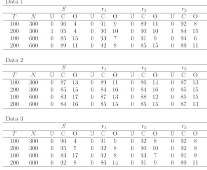
number of groups, the number of group-specific pervasive factors and the size of the regularization parameter. We set the possible numbers of group-specific pervasive factors to range from zero to eight. Thus, the maximum number of group-specific pervasive factors was set to eight. The number of groups ranges from two to four. Possible candidates for the regularization parameterκ are κ={10,1,0.1,0.01,0.001}. Table 1 reports the percentage of under-, correct, and overidentified values for the proposed Cp criterion under the three data-generating models. With respect to the
number of groups, we can easily calculate the percentages of under- (U), correct (C), and overidentified (O) values. The percentages with respect to the number of group-specific factors are calculated under the condition that the number of groups is correctly selected. This is because of the difficulty of the matching between the true number of group-specific factors and the selected number of group-specific factors when the selected number of groups and true number of groups are different. As shown in the tables, the proposed Cp criterion is capable of selecting the true number of groups as
well as the true number of group-specific pervasive factors.
Finally, we discuss the regression coefficient estimation results. The simulation re-sults for the parameter estimates of ˆβ are reported in Table 2. Because the length of ˆ
βis very long, we report the estimation results for the true predictors ( ˆβ1,βˆ2,βˆ3)′, and
that for the first three wrong predictors ( ˆβ4,βˆ5,βˆ6). We point out that the
As shown in Table 2, the parameters are well estimated in the simulation studies. Furthermore, the accuracy improves as the size of the panel increases.
We point out that the proposed method implicitly assumes that each group should not be completely overlapped. Additional experiments that we have performed suggest that group separation, coming from the observable parts of Xiβ, or coming from the
group-specific factor structures fgi,tλgi, or both, is important. In summary, our
simu-lation results show that the proposedCp criterion works well in selecting the number of
groups and the number of group-specific pervasive factors. Furthermore, the regression coefficients ˆβ are estimated very well.
7
Analysis of US mutual fund styles
A mutual fund is a portfolio of financial assets managed by a professional institution on behalf of its clients. It is common that the professional institutions manage clients’ assets according to a particular investment style, which defines the nature of the fund. There are well known criteria that define the investment styles, for example, “Value” and “Growth”, “Large Cap” and “Small Cap”, etc. To provide investors with a guide to the mutual funds market, some professional institutions issue classifications of existing mutual funds according to the investment objectives stated by the funds. Practically, one may rely on the institutional classification scheme; however, it does not always provide consistent and representative peer groups of fund styles. In this section, we aim at grouping mutual funds and identifying their styles by analyzing the time series of past returns of each mutual fund.
7.1
Data and model
We analyzeT = 85 monthly returns yit for N = 536 US mutual funds, collected from
Thomson Financial Datastream database for October 2003 to October 2010. Here we focus mainly on the four mutual fund styles: Small Capital & Growth, Large Capital & Growth, Small Capital & Value, and Large Capital & Value.
The specified model is
yit = β0+
7
X
s=1
yi,t−sβs+
7
X
w=1
ui,twβw+M kttβM kt+HM LtβHM L+SM BtβSM B
+LT RtβLT R+ST RtβST R+M omtβM om+f′gi,tλgi,i+εit,
i = 1, . . . , N, t = 1, . . . , T,, where ui,tw = Pwk=0I(yi,t−k > 0) is the number of past
months such that a positive return is realized, and I(·) is an indicator function that takes the values 1 or 0. Therefore ui,tw is the cumulative sum of the months with
ratio (HML), and the third based on excess return (Mkt) on the market. We also used the long-term return reversal factor (RTR), the short-term return reversal factor (STR), and the momentum factor (Mom). These factors are obtained from the Fama and French database.
7.2
Results
We applied the proposed model selection criterion, Cp, to select simultaneously the
number of groups, the number of group-specific pervasive factors and the size of the regularization parameter. We set the possible numbers of group-specific pervasive fac-tors to range from zero to eight. Thus, the maximum number of group-specific pervasive factors was set to eight. The number of groups ranges from one to nine, i.e.,Smax= 9.
Possible candidates for the regularization parameterκ are κ={10,1,0.1,0.01,0.001}. As a result, the selected number of groups is ˆS= 6. A two-way table of the grouping output against the four mutual fund styles is provided in Table 3. The two classification schemes appear to be similar in several respects, although the classification based on the mutual fund names is more parsimonious than in our grouping. Memberships overlap considerably for the constructed groups and the classification by name. The distribution of the funds’ memberships is easy to interpret according to mutual fund names. For example, the constructed group 6 (G6) corresponds to Small Capital & Growth. However, Small Capital & Growth mutual funds are divided into other groups. Group 1 contains 64 Small Capital & Growth mutual funds and the “Growth” factor plays a main role. Groups 2 and 4 contain 19 and 14 Small Capital & Growth mutual funds and the “Small” factor is the most important characteristic. Group 3 mostly contains Large Capital & Growth mutual funds. Therefore, both “Large” and “Growth” factors may characterize the fund returns. Group 5 is the group in which “Large” and “Value” factors might be related. The comparisons in Table 3 show the potential of the proposed method. The agreements between the two schemes suggest that our procedure succeeds in recognizing the fundamental differences among funds.
The selected numbers of group-specific pervasive factors arer1 = 4, r2 = 3, r3 = 3,
r4 = 3, r5 = 2, r6 = 3, respectively. Therefore, there are group-specific pervasive
fac-tors that explain the mutual fund returns within the groups. The estimated regression coefficients {βˆs,βˆw|s, w = 1, ...,7} are estimated as zero, which partially implies that
the return prediction from the historical information is difficult. We found that the estimated regression coefficients on the style factors {βˆM kt,βˆHM L, ...,βˆM om} are also
zero. This result makes sense because the investment styles (i.e., a sensitivity to the set of investment style factors {M ktt, HM Lt, SM Bt, LT Rt, ST Rt, M omt}) are
differ-ent among the set of 536 mutual funds. In Section 8, we introduce the model with heterogeneous regression coefficients that vary over the groups.
the absolute value of the correlations are larger than 0.18, 0.22, and 0.29, the corre-sponding significance levels are 10%, 5% and 1%, respectively. From the table, we make the following observations. First, the Mkt factors are mainly related to the first group-specific pervasive factor for all six groups. In particular, the magnitude of the correlation is the highest among those with other styles. Second, the SMB factor is highly related to the first group-specific pervasive factor of group 1, while it has a very low correlation with the factors of other groups. Third, the HML factor has high correlations with the group-specific pervasive factors of groups 1 and 2. Fourth, the momentum factor, short-term return reversal factor, and long-term return reversal fac-tor also play an important role as the high-level correlations show. Fifth, some of the estimated group-specific pervasive factors have low correlations with the six observable investment styles (Mkt, HML, SMB, STR, LTR, and Mom). For example, the second group-specific pervasive factor of group 5 has very low correlation with these variables. It would be interesting to explore some possible investment styles that have a large correlation with such factors. Overall, the estimated group-specific pervasive factors vary over the groups.
8
Heterogeneous group-specific coefficients
The model (1) can be extended to the heterogeneous group-specific coefficients
yit=x′itβgi +f
′
gi,tλgi,i+εi,t, i= 1, . . . , N, t = 1, . . . , T, (9)
where thepi×1 vectorβgi contains the unknown regression coefficients for each group. The regression coefficient is group-specific, but not individual-specific. It may be of interest to extend the model to individual-dependent coefficients, which is not studied in this paper. The model assumptions are the same as in Section 2.1, except we need to modify Assumption D as follows.
Assumption D′: Observable predictors
(D1′) For the matrices D
j, Ej and Lj defined in Assumption D of Section 2.1, we
assume
Dj −L′jEj−1Lj
is positive definite for all Fj such that Fj′Fj/T =I and for all groupings with a
positive fraction of membership. Assumption D2 is maintained.
(D2′): The vector of predictor x
it satisfies max1≤i≤NT−1kXik2 = Op(Nα) with α <
1/16. We also assumeN/T2 →0.
In D2′, we now require α < 1/16 instead of α < 1/8. Again, this is much weaker
than assuming xit has exponential tails. Assumption D′ ensures the existence of the
8.1
Estimation procedure
Under a given number of groupsS, number of factors r1, ..., rS, and size of the SCAD
penaltyκ, our estimator{βˆ1, ...,βˆS,G,ˆ Fˆ1, ...,FˆS,Λˆ1, ...,ΛˆS}is defined as the minimizer
of
LN T(β1, ...,βS, G, F1, ..., FS,Λ1, ...,ΛS)
=
S
X
j=1
X
i;gi=j
kyi−Xiβgi−Fgiλgi,ik
2+
S
X
j=1
N T ·pκ,γ
¡ |βj|¢,
subject to the constraints on the factor and factor loading matrix imposed in Section 2.
Given the group membership G and the values of regression coefficient βj, the factor structures are estimated as described in Section 2. Given the group membership
G and the factor structures, the regression coefficients βj can be updated. It is easy to see that, for any given values ofβj andFjλj,i (j = 1, ..., S), the optimal assignment
for each individual unit is: g∗
i = argminj∈{1,...,S}T−1kyi−Xiβj −Fjλj,ik2+pκ,γ(|βj|).
The estimates ofβ, {Fj,Λj; j = 1, ..., S}, and G={g1, ..., gN} depend on each other,
the estimators are obtained by almost the same procedures as in Section 2.
8.2
Asymptotic results
Here, we use{F0
j, j = 1, ..., S}to denote the true parameter values of the group-specific
factors Fj that satisfies Assumptions A, B, C, D′ and E. As N and T increase, we
claim that the estimated factors are consistent in the sense of some averaged norm, which will be specified below. We have the following theorem.
Theorem 6 : Consistency. Under Assumptions A, B, C, D′ and E, κ → 0 and
min{Nj, T} ×κ→ ∞ as T, N → ∞, the estimators βˆj are consistent
kβˆj−β0jk=op(1), for j = 1, ..., S,
In addition,{Fˆj, j = 1, ..., S} are consistent in the sense of
T−1/2kFˆj −Fj0Hjk=op(1),
where Hj−1 =Vj,NjT(F
0
jFˆj/T)−1(Λ0
′
j Λ0j/Nj)−1, and Vj,NjT satisfies
1
NjT Nj X
i;ˆgi=j
(yi−Xiβˆj)(yi−Xiβˆj)′
Fˆj = ˆFjVj,NjT.
The estimates of β1, ..,βS, {Fj,Λj; j = 1, ..., S}, and G ∈ {g1, ..., gN} depend
on each other, and we therefore denote the estimator of group membership ˆgi as
ˆ
gi( ˆβ1, ...,βˆS,F ,ˆ Λ) in the following theorem. The following theorem shows that theˆ
estimated group membership converges to the true group membership as T and N
Theorem 7 : Consistency of the estimator of group membership. Suppose that the assumptions in Theorem 6 hold. Then, for all τ >0 and T, N → ∞, we have
P
Ã
sup
i∈{1,...,N}|
ˆ
gi( ˆβ1, ...,βˆS,F ,ˆ Λ)ˆ −gi0|>0
!
=o(1) +o(N/Tτ),
where Fˆ ={Fˆ1, ...,FˆS} and Λ =ˆ {Λˆ1, ...,ΛˆS}.
Let us define ˜β1, ...,β˜S,F˜1, ...,F˜S,Λ˜1, ...,Λ˜Sas the infeasible version of our estimator
where group membership is fixed to its populationG0. It is defined as the minimizer
ofLN T(β1...,βS, G0, F1, ..., FS,Λ1, ...,ΛS) subject to the usual constraints. Theorem 7
shows that, under a certain condition, our estimator{βˆ1, ...,βˆS,Fˆ1, ...,FˆS,Λˆ1, ...,ΛˆS}is
asymptotically equivalent to the infeasible estimates ˜β1, ...,β˜S,F˜1, ...,F˜S,Λ˜1, ...,Λ˜S as
N andT tend to infinity. If for someb >0,N/Tb →0 as bothN andT tend to infinity
simultaneously, the proposed estimator ˆβj, ˆFj(j = 1, ..., S) and the infeasible estimator
˜
βj, ˜Fj (j = 1, ..., S) with known population groups are asymptotically equivalent.
In the next theorem, we provide the asymptotic normality and the variable selection consistency. Letβ0j = (β0j,1′,β0j,2′)′ be the true parameter vector such thatβ0
j,2 =0. We
denote the corresponding estimate as ˆβj = ( ˆβ′j,1,βˆ′j,2)′. We show thatP( ˆβ
j,2 =0) will
converges to 1 as N, T → ∞. Also, the parameter estimate ˆβj,1 is the asymptotically normal.
Assumption F′
LetXi,βj6=0 be the submatrix ofXicorresponding to columns of the nonzero elements of the parameter vectorβj. Letqj be the number of nonzero elements ofβj (j = 1, ..., S).
For the nonrandom positive definite matrixJ0(Fj0),
1 p
NjT
X
i:g0
i=j
Zj,i(Fj0)′εi →dN(0, J0(Fj0)),
whereZj,i(Fj0) =Xi,β′ 6=0MF0
j−N
−1
j
P
k:g0
k=jcj,kiX
′
k,β6=0MF0
j, withcj,ki =λ
0′
g0
k,k(Λ
0′
j Λ0j/Nj)−1λ0g0
i,i, and J0(Fj0) is the probability limit of
ˆ
J(Fj0) = 1
NjT
X
i:g0
i=j X
ℓ:g0
ℓ=j
Zj,i(Fj0)′E[εiε′ℓ]Zj,ℓ(Fj0).
Then, we have the following theorem.
Theorem 8 : Asymptotic normality and variable selection consistency
As-sume that the assumptions in Theorems 6 and 7 andF′ hold. Then, p
NjT( ˆβj,1−β0j,1)
p
NjT( ˆβj,1−β0j,1) →d N(vj0, Vβ(Fj0)). Moreover, the following variable selection
con-sistency holds:
P( ˆβj,2 =0)→1 N, T → ∞,
for j = 1, ..., S. Here, the variance–covariance matrix Vβj(F
0
j) is
Vβ(Fj0) =D0(Fj0)−1J0(Fj0)D0(Fj0)−1,
where D0(Fj0) is the probability limit of
ˆ
D(Fj0, κT) =
1
NjT
X
i:g0
i=j "
Xi′MF0
jXi− 1
Nj
X
k:g0
k=j
cj,kiXi′MF0
jXk #
+ 1
NjT
Σj(κT),
withΣj(κT) = diag
©
p′
κT,γ(|βj,1|)/|βj,1|, . . . , p
′
κT,γ(|βj,qj|)/|βj,qj| ª
, whereqj is the number
of nonzero elements of β0j, and vj0 is the probability limit of
s
T
Nj ×
ˆ
D(Fj0, κT)−1ηj+
r
Nj
T ×Dˆ(F
0
j, κT)−1ζj,
where
ζj =− 1
NjT
X
i:g0
i=j X
k:g0
k=j
Xi′MF˜jΩkFj0
Ã
F0
j
′
F0
j
T
!−1 µΛ′
jΛj
Nj
¶−1
λg0
i,i,
ηj =− 1
NjT
X
i:g0
i=j X
k:g0
k=j
(Xi−Vj,i)′Fj0
Ã
F0
j
′
F0
j
T
!−1 µΛ′
jΛj
Nj
¶−1
λg0
k,k µ
E[ε′
iεk]
T
,
with cj,ki =λ0
′
g0
k,k(Λ
0′
j Λ0j/Nj)−1λ0g0
i,i, and Vj,i=N
−1
j
P
k:g0
k=jcj,kiXk.
The proof of the theorem is given in the Appendix.
8.3
Determining the number of groups/factors
Taking into account the consistency of the proposed model selection criterion, we again suggest minimization of the predictive measure
1
N T
S
X
j=1
X
i;giˆ=j
° °
°yi−Xiβˆgi −Fˆgˆiλˆˆgi,i ° ° °
2
+ ˆb(k1, ..., kS, κ).
Theorem 9 Under the assumptions of Theorems 6-8, the penalty term is
ˆb(k1, ..., kS, κ) =
S
X
j=1
1
N Ttr
£
Kj,xVβ(Fj0, κ)
¤ +
S
X
j=1
kj ×gj(T, N1, ..., NS),
whereKj,x= 2
P
i;gi=jX
′
i,βˆj6=0Xi,βˆj6=0/(NjT)withXi,βˆj6=0 being the submatrix ofXi such
that the corresponding columns contain a nonvanishing component of the parameter estimate, and Vβ(Fj0, κ) = ˆD(Fj0, κ)−1Jˆ(Fj0) ˆD(Fj0, κ)−1. Here Jˆ(Fj0) and Dˆ(Fj0, κ) are
defined in Assumption F′ and Theorem 8. The function g
j(T, N1, ..., NS) satisfies (a)
gj(T, N1, ..., NS)→0 and (b) min{N, T} ×gj(T, N1, ..., NS)→ ∞ as T, N → ∞.
Using the same investigations in Section 4, we have the following criterion:
Cp(k1, ..., kS, κ) =
1
N T
S
X
j=1
X
i;ˆgi=j
kyi−Xiβˆˆgi −Fˆˆgiλˆgˆi,ik
2
+
S
X
j=1
1
N Ttr
h
Kj,xVβ( ˆFj, κ)
i +
S
X
j=1
kjσˆ2
Nj
N
µ
T +Nj
T Nj
log (T Nj), (10)
where ˆσ2is a consistent estimate of (N T)−1PS
j=1
P
g0
i=jkyi−Xi ˆ
βg0
i− ˆ
Fg0
i ˆ
λg0
i,ik
2. Under
the criterion, the numbers of factors are consistently estimated.
Similar to the Cp criterion, ˆσ2 provides proper scaling for the penalty term. In
applications, it can be replaced by its consistent estimator. Finally, we provide the fol-lowing theorem, which states that the value ofScan also be identified as the minimizer of the preceding information criterion.
Theorem 10 LetSˆbe the minimizer of the proposedCp(k1, ..., kS, κ)criterion in (10).
The determined number of groups, Sˆ, converges in probability to the true number of groups S0 as T, N → ∞.
9
Analysis of China’s mainland stock markets
The relative strengths of industry versus exchange-listed effects can be of major impor-tance for equity portfolio managers. If market-listed effects dominate, then primary consideration can be given to the market allocation decision. In contrast, if China’s mainland stock market integration is reducing the distinction between markets, then an industry-first investment process may be more appropriate.
In these markets, two types of shares are traded, namely A- and B-shares. Al-though A- and B-shares are listed and traded in the mainland market, the former are denominated in RMB and were originally traded only among Chinese citizens, whereas the latter are denominated in foreign currencies and were originally traded among non-Chinese citizens or among non-Chinese residing overseas. The non-Chinese government launched the qualified foreign institutional investors (QFII) policy in 2003 and introduced for-eign investors into the domestic A-share market. Although Chinese mainlanders have been eligible to trade B-shares with legal foreign currency accounts since March 2001, the mainlanders may prefer to trade only in A-shares because of the currency barrier. It therefore seems plausible that the underlying asset return structure of A-shares is different from that of B-shares.
This paper investigates empirical questions such as the following: How many groups exist in the stock markets in mainland China? How many group-specific pervasive factors exist in the stock markets in mainland China? What types of observable risk factors explain the stocks in each group? Finally, how can the unobservable factors be understood in terms of observable variables in the economy?
9.1
Data
We use monthly excess returns of the Shanghai and Shenzhen stock exchanges from Standard & Poor (S&P)’s Datastream Database. We consider an approximately eight-year sample, covering March 2002 to October 2010, and systematically exclude stocks with missing returns data. We calculate excess returns by subtracting the interest rate on the one-month interbank offer rate from the individual stock returns. The above filtering procedure yields 1,039 A-share firms and 102 B-share firms, listed on the Shanghai stock exchange and the Shenzhen stock exchange respectively.
9.2
Result
We fit the model (9) by minimizing the objective function. Then, we applied the proposed model-selection criterion,Cp, to select simultaneously the number of groups
S, the number of group-specific pervasive factors, and the size of the regularization parameter κ. We set the maximum number of groups to Smax = 20. The possible
number of group-specific pervasive factors rj range from 0 to 20. Although we set the
maximum number of possible factors more than 20, this number may be enough based on the stock market analysis of other countries (see for e.g., Fama and French (1993)). Possible candidates for the regularization parameterκ are κ={10,1,0.1,0.01,0.001}. The estimated number of groups is ˆS = 6 because this achieved the smallest value of the proposed model-selection criterion,Cp. This suggests that there are approximately
six groups in the Chinese mainland stock markets. Hereafter we denote each of these six groups as G1∼G6. As the market/industry classifications are known, a two-way table of the estimated group membership ˆgi against these classifications is provided
in Table 5. The nominal classification schemes are based on: 1. Location of stock exchanges, 2. Types of share (A-share or B-share), and 3. Industry. The estimated group memberships appear to be more related to the A-share/B-share classification rather than to the other two factors. Group G5 is comprised of almost exclusively (approximately 90%)B-shares. Although group G3 also containsA-shares, we suspect that the international investors are also buying the A-shares included in group G3. This indicates that the investors may first consider the types of share (A-share/B-share) rather than the industry or stock exchanges.
The estimated number of group-specific pervasive factors is: 3 group-specific perva-sive factors with respect to groups G3 and G5, 2 group-specific pervaperva-sive factors with respect to groups G2, G4 and G5, and 1 group-specific pervasive factor with respect to group G1. Although the group G1 is a mix of A-shares and B-shares, the number of group-specific pervasive factors of this group is smaller than that of group G5.
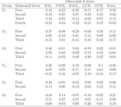
The estimated group-specific pervasive factors do not have an immediate economic interpretation. We therefore further explore the economic meanings of the estimated factors in each group. In this paper, we regress the estimated group-specific pervasive factors ˆfjk,t (j = 1, ..., S;k = 1, ..., rj) on some economic factorszt; ˆfjk,t=z′tγjk+ejk,t,
and then conduct statistical significance tests of the least squares estimate ˆγjk.
the value premium. SMB measures the historic excess returns of small caps over big caps. These variables are computed using Chinese data.
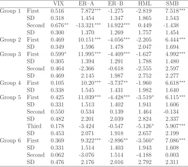
Table 6 summarizes the results. In Table 6, for each factor, the first row corre-sponds to the estimated regression coefficients, whereas the second row correcorre-sponds to the standard deviations. In the table, stars (***), (**) and (*) mean that the estimated regression coefficient is statistically significant at the 1%, 5%, and 10% levels, respec-tively. We can see from Table 6 that for the first group-specific pervasive factor, the first element of fk,t relates to the market excess returns of A-shares. This is expected because all groups contain many shares, and even for group G5, the number of A-shares exceeds the number of B-A-shares. Furthermore, the size factor SMB also relates to the first group-specific pervasive factor. Contrary to findings for the US market, the book-to-market ratio factor (HML) is weakly related to the estimated factors. As we expected, the group-specific factors of group G1 relate strongly to the market excess returns of B-shares as well as A-shares. With respect to VIX, the group-specific fac-tors of group G1 an G3 are weakly related. We suspect that the invesfac-tors in B-shares are monitoring the volatility index. Overall, we can see some differences among the group-specific pervasive factors.
From Theorem 8, we can implement a statistical significance test for the estimated regression coefficients ˆβk k = 1, ...,6. Thus, we can check whether the regression coef-ficients ˆβk for each security are statistically significant. Table 7 shows the statistically significant observable risk factors for each group. In the table, stars (***), (**) and (*) mean that the observable risk factor is statistically significant at the 1%, 5%, and 10% levels, respectively.
10
Conclusion
The proposed panel data modeling procedures provide a flexible yet parsimonious ap-proach to capturing unobserved heterogeneity. The regression parameters, unobserv-able factor structure, and group membership were all estimated jointly. The lasso approach allows us to implement the model estimation procedure easily. We provided a novel argument of consistency, which is the most difficult part to obtain. We also proposed a Cp-type model selection criterion. The Monte Carlo results showed that
the proposed procedure performed well. The proposed procedure is then applied to the study of US mutual fund style analysis. A two-way table of the grouping output against the four mutual fund styles showed that our procedure succeeds in recognizing the fundamental differences among funds.
We also consider heterogeneous regression coefficients that varies over the groups. Asymptotic normality and the variable selection consistency of the estimated hetero-geneous coefficients were again obtained. To determine the number of group-specific factors, the magnitude of the regularization parameter and the number of groups, we again developed aCp-type model selection criterion for selecting these quantities.