Development of models for forest variable estimation from airborne laser scanning data using an area based approach at a plot level

JOURNAL OF FOREST SCIENCE, 62, 2016 (3): 137–142

doi: 10.17221/73/2015-JFS

Development of models for forest variable estimation

from airborne laser scanning data using an area-based

approach at a plot level

J. Sabol

_{, D. Procházka}

_{, Z. Patočka}

1_{Department of Forest Management and Applied Geoinformatics, Faculty of Forestry}

and Wood Technology, Mendel University in Brno, Brno, Czech Republic

2_{Department of Informatics, Faculty of Business and Economics, Mendel University in Brno,}

Brno, Czech Republic

ABSTRACT: Airborne laser scanning (ALS) is increasingly used in the forestry over time, especially in a forest in-ventory process. A great potential of ALS lies in providing quick high precision data acquisition for purposes such as measurements of stand attributes over large forested areas. Models were developed using an area-based approach to predict forest variables such as wood volume and basal area. The solution was performed through developing an object-oriented script using Python programming language, Python Data Analysis Library (Pandas), which represents a very flexible and powerful data analysis tool in conjunction with interactive computational environment the IPython Notebook. Several regression models for estimation of forest inventory attributes were developed at a plot level.

Keywords: Python; Fusion; forest inventory; linear regression; Norway spruce

Forest inventory is the basis for a forest information system for forest planning and management feedback control. Forest inventories generally use random or systematic sampling schemes. In both methods, a limited number of plots are inventoried because this work is both costly and time-consuming. Field mea-surements can only be performed in areas that are ac-cessible to field crews (Poleno et al. 2007).

Therefore, remote sensing has shown the im-mense potential to provide quick and accurate measurements of stand attributes over vast areas at a much lower cost than with traditional inventory practices. Using remote sensing data, coupled with a small number of field measurements, can thus be an effective solution to overcoming the afore-mentioned drawbacks of field measurements, while providing accurate and timely information on sev-eral key forest attributes.

The most frequently exploited remote sensing tech-nology in forest applications is indisputably airborne

laser scanning (ALS), also referred to as light detection and ranging (LiDAR). Its potential for forest attribute estimation at several scales is widely acknowledged. LiDAR-based forest inventories employ two major methods, depending on the unit to be estimated. In the individual tree detection (ITD) approach, as the name itself suggests, the aim is to detect and delineate single trees (e.g. Hyyppä, Inkinen 1999; Holmgren, Perrson 2004; Popescu et al. 2014). Once the trees are detected, attributes are extracted or modelled for each tree from ALS observations. On the other hand, in the area-based approach (ABA), also referred to as canopy height distribution method, the unit is an area of a certain fixed size. The mean values of forest stand variables are estimated using statistical correlations between explanatory variables, derived from LiDAR point cloud, and forest stand variables measured at a plot level (e.g. Naesset 2002, 2007; Packalén, Maltamo 2007). ABA has shown to provide reliable estimates of growing stock. LiDAR-based estimates

for total characteristics are even more accurate than inventory results based on visual assessment and sub-jective field measurements (Peuhkurinen 2011).

The aim of this study was to develop models of forest stand attributes from ALS data using the lat-ter method. The solution was performed through developing an object-oriented script using Python programming language, Python Data Analysis Li-brary (Pandas, Lambda Foundry, New York, USA; McKinney et al. 2015), which represents a very flexible and powerful data analysis tool in conjunc-tion with interactive computaconjunc-tional environment the IPython Notebook (Fernando Peréz, Berkeley, USA; Peréz, Granger 2007).

MATERIAL AND METHODS

LiDAR data. High density LiDAR data were col-lected at the beginning of September 2014 in the territory of the Training Forest Enterprise (TFE) called Masaryk Forest Křtiny. TFE Masaryk For-est Křtiny represents a continuous complex of for-est lands linking with the northern edge of Brno, with an area of 10,228 ha. The forests are situated at altitudes ranging from 210 to 575 m a.s.l. and are characterized by a variety of natural conditions. Mapping of this relatively small area, dominated mostly by mixed woods with 46% of coniferous and 54% of deciduous tree species, revealed 116 forest types situated in 4 forest altitudinal zones. Mean annual temperature of 7.5°C and mean annual pre-cipitation of only 610 mm are limiting factors. To-pography is very broken with deep-incised valleys and glens, especially those of the Svitava River and the Křtinský potok Brook. The parent rock is com-posed of granodiorites, Culmian greywackes and limestone. About a third of the TFE area is situated in the Protected Landscape Area of the Moravian Karst. Main local tree species are spruce, pine, larch for conifers and beech and oak for broadleaved species (TFE Masaryk Forest Křtiny, 2002–2008).

Scanning was performed with a Leica ALS70-CM scanner (Leica Geosystems, Heerbrung, Switzer-land) mounted on the aircraft OK-EKT Cessna 206 Turbo Stationair (Cessna Aircraft Co., Wichita, USA). The used scanning angle was 24° with an av-erage pulse density of 7.8 pulses/m2 _{in the ETRS-89}

UTM 33N coordinate system. Filtering and classi-fication of the LiDAR point cloud was performed in TerraSolid TerraScan software (Terrasolid, Hel-sinky, Finland) for Bentley MicroStation. Conse-quently, LiDAR data together with field plot data were used for calculating point cloud metrics using

Fusion software (Department of Agriculture, For-est Service, University of Washington, Washington, USA; McGaughey 2014).

Field plot data. Field data collection took place from the beginning of the year 2015 in the TFE Masaryk Forest Křtiny in Forest District Habrůvka. 39 circular plots with a radius of 12.62 m were es-tablished in spruce dominated sites situated mostly in the 4th _{forest altitudinal zone and within 3 forest}

stand groups (35, 41, 45), but prevailing majority pertained to management of nutrient sites of me-dium altitudes (45). The age of stands ranged from 60 to 130 years, with a predominant proportion of stands older than 100 years.

The centres of sample plots were measured using a Topcon HiPer Pro GNSS receiver (Topcon, To-kyo, Japan) with applied real-time kinematic (RTK) corrections to enhance the precision of the posi-tion. The measurement took 20 minutes at 5 sec-ond intervals. All the threshold values of GNSS re-ceiver were left at default settings (elevation mask threshold – 5°, signal-to-noise-ratio threshold – 99, dilution of precision threshold – 99). The height of the antenna was 2 meters.

Diameter at breast-height (DBH) was measured for all trees with DBH > 7 cm and heights for each tree. Furthermore, basal area was calculated and volume estimated for each field plot using volume equations according to Petráš and Pajtík (1991).

Data pre-processing. Once the coordinates for all plots are available, the last step in the data prepa-ration process consists of subsetting the LiDAR re-turns that correspond to each field plot. During the subsetting process, LiDAR data are normalized to the ground surface so the returns are expressed in terms of heights above the ground. After subsetting the LiDAR plot equivalents, the last step consists in calculating a set of cloud metrics variables for each of the plots. Metrics are computed using point el-evations and intensity values. Output is formatted as a comma separated value (CSV). Each record in the output table has a set of variables that together de-scribe the vertical distribution of the LiDAR points within the plot. These variables were used as the pre-dictor variables in the linear regression modelling.

Predictive models were developed according to general principles of LiDAR based model building as McGaughey (2014) proposed:

(1) models should have as few parameters as possible; (2) simple explanations should be preferred to complex

explanations;

(3) experiments relying on few assumptions should be preferred to those relying on many;

(4) most predictive LiDAR based models should not have more than three variables generally represen-ting some form of the three metrics listed below:

(i) one related to height; (ii) one related to canopy cover; (iii) one from descriptive category.

The script is designed for interactive computa-tional environment the IPython Notebook (Peréz, Granger 2007), in which it is possible to combine not only code execution but also text, mathemat-ics and plots. Data manipulations were performed using the open source library Pandas for efficient, intuitive and flexible input data handling by means of data frame structures. For building the regression model and for subsequent tests and diagnostics a Python module Statsmodels (Josef Perktold, Mon-treal, Canada) was used (Perktold et al. 2013). A Python library Matplotlib (John D. Hunter, Chicago, USA, Hunter et al. 2015) was used for interac-tive displaying of charts in the IPython Notebook environment.

RESULTS

Implementation

Input data consist of two CSV files, the one with measured variables for each plot and the other con-taining calculated point cloud metrics using the Fusion software.

The script itself consists of two classes. Along with the instantiation of the first class, by setting the paths for input tables as the first and second argument, additional arguments described in class documentation have to be set. Desired forest in-ventory variable for modelling as a string is the first one (e.g. G – basal area, V – volume), the other two are related to correlation analysis – method for calculating the correlation coefficient as a string (Pearson’s correlation coefficient is recommended) and threshold value as a number, determining the acceptance level of the correlation coefficient of point cloud metrics for modelling.

After the class instantiation, the initialization meth-od creates instances from both input tables adding

them to the Pandas format data frame, and further-more calls each private method, constructed for data converting, cleaning and handling. The first public method being actually called by the user is the regres-sion model building itself. According to general prin-ciples of the regression model building mentioned above, one to three independent variables can be se-lected from a list of point cloud metrics printed as a table along with the instantiation. Cloud metrics for model fitting are set manually as numbers, accord-ing to indices in the printed table or an optimization method could be utilized as described below in a contiguous subchapter. The returned result of fitted model uses attributes and methods of Statsmodels re-gression result described in its documentation which are obtained by means of code completion function-ality in the IPython Notebook environment. It is used by typing the name of the result object with dot right after it and by pressing the tabulator key. Then the drop-down list of attributes and methods for the re-sult object emerges (e.g. result.summary), where the result is an object created by the method for fit-ting a regression model and summary is a Statsmo-dels method, which produces an “human-readable” output of regression analysis.

The second class uses the resulting regression model as its input parameter and contains private methods for plotting and a number of public meth-ods for regression diagnostics (e.g. Breusch-Pagan test, Goldfeld-Quandt test), which are called man-ually by means of the aforementioned code com-pletion functionality in the IPython notebook en-vironment. The plots consist of partial regression plots, influence plot, QQ-plot, leverage-resid2 _plot

and Cook’s distance plot. All plots are displayed au-tomatically right after the instantiation of the diag-nostics class.

Model building

The predictor variables were selected either man-ually from a list of cloud metrics printed along with the instantiation of the first class, or by means of an optimization method that could be chosen from the list of public methods of a class. According to prin-ciples outlined in McGaughey (2014), this meth-od creates all possible combinations of pairs and triples of accepted cloud metrics and consequently constructs a regression model for each combina-tion. The result of this method is a table with ID numbers of combinations as rows and assessment criterions (R2_{, F-test, AIC, etc.) as columns. The}

reli-ability can then be selected for further modelling and evaluated by the regression diagnostics as well.

Several regression models for forest inventory variables were developed and regression triplet was tested. All the selected models consisted of three or two predictor variables. Each model was validated and based on the tests performed, no errors were drawn that would affect their credibility. The follow-ing formulas may be tested for further modellfollow-ing of forest inventory variables on the whole inventory area using the ArcGIS software (ESRI, Redlands, USA).

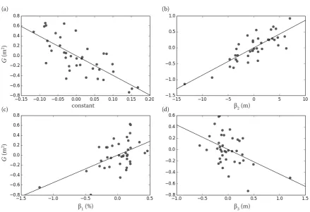
Model for basal area (Fig. 1)

The model for basal area G (m2_{), R}2 _{= 0.79, RMSE =}

1.2, RMSE (%) = 50.2, bias = 0.19 (Eq. 1):

G = –3.9456 + 0.5536 × β₁ + 0.0861 × β₂ – 0.433 × β₃ (1)

where:

β₁ – cubic mean of height of all points within the point cloud (m),

β₂ – percentage of all returns above the mean height of all returns within the point cloud above surface (%), β₃ – height of returns in the 60th _{percentile (m).}

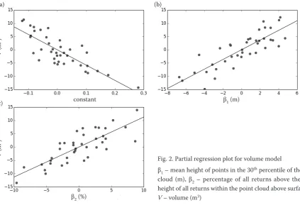
Model for volume (Fig. 2)

The model for volume V (m3_{), R}2 _{= 0.84, RMSE =}

17.77, RMSE (%) = 54.16, bias = 2.85 (Eq. 2):

V = –57.6938 + 1.826 × β₁ + 1.1315 × β₂

where:

β₁ – mean height of points in the 30th _{percentile of the}

point cloud (m),

β₂ – percentage of all returns above the mean height of all returns within the point cloud above surface (%).

DISCUSSION

LiDAR point cloud metrics related to height, the coefficient of variation of height, and the density of cover were used for developing the models to predict stand attributes using ABA. Subsets of these met-rics were used as independent variables in ordinary least-square regression. This is a common approach which has been used in many other studies (Naes-set 2002, 2004; Lim, Treitz 2004). The strength of relationships between point cloud metrics and forest inventory attributes is predicated on the capability of LiDAR data to accurately characterize canopy height

Fig. 1. Partial regression plot for basal area model

β₁ – cubic mean of the height of all points within the point cloud (m), β₂ – percentage of all returns above the mean height of all returns within the point cloud above surface (%), β – height of returns in the 60th _{percentile (m), G – basal area (m}2₎

G

(m

2)

G

(m

2)

β₁ (%) β₃ (m)

(c) (d)

(a) (b)

and density. Therefore, ensuring that non-canopy re-turns are separated from canopy rere-turns is essential to develop models. In most studies, non-ground returns below a 2-m height threshold were excluded from the calculation of point cloud metrics (Naesset 2002). The 2-m threshold has been applied also in this case. Research indicates that the 2-m threshold is appropri-ate in the conditions of mature boreal forests, hence all of the sample plots were located in the coniferous forest type dominated by Norway spruce.

Metric selection was done manually by an intuitive approach as recommended by White et al. (2013) or by employing an optimization method as described above in the preceding chapter. Metric selection may suffer from either overfitting or multicollinearity (Chen et al. 2007). An overfitting problem was irrel-evant after all, since only three or less cloud metrics were used as predictors of the model. A strong inter-correlation between candidate cloud metrics gener-ated from LiDAR data is one of the ABA drawbacks. Multicollinearity does not reduce the predictive pow-er or reliability of the model as a whole, but the model may not give valid results. Therefore, metrics with high correlation between each other were excluded. Dropping a predictor can be sometimes actively mis-leading, but in this case, excluding the predictors is a somewhat reasonable thing to do, since many of the cloud metrics are measuring more or less the same thing. As well, principal component analysis can be used to set a small set of relevant metrics, but the in-tercorrelation of many LiDAR cloud metrics still

un-dermines this approach. This problem was partially solved by centring the independent variables. This phenomenon was caused particularly by a small sam-ple of observations, therefore it was tested right along with fitting the model, so the intercorrelated metrics could be replaced and the model refitted. There is also a risk in extrapolating the modelled relationship beyond the range of the field collected data, due to the lack of field plot data. Notwithstanding that field work is both costly and time-consuming, it is high-ly recommended to obtain more data from ground measurements for further testing.

The results indicate that the use of LiDAR data is a viable data source for generating accurate estimates of forest variables such as wood volume or basal area. It appears that the LiDAR-based cloud met-rics, based upon the height distribution of LiDAR measurements, capture structural information re-lated to quantitative canopy characteristics. In spite of the considerable variation around canopy height quantiles and in laser sampling density of the 500 m2

plots, the coefficients of determination (R2_{) for}

vol-ume of 0.84 and basal area 0.79 seem to correspond more or less to previous findings.

Means et al. (2000) reported R2 _{for basal area and}

volume of 0.94–0.95 and 0.95–0.97, respectively, for 2500 m2 _{plots, which is slightly better than}

find-ings introduced in this study. On the other hand, the precision seems to be fully corresponding with the size of the plots and their number, as outlined in Naesset (2002), where 88 circular plots with the

V

(m

3)

V

(m

3)

β₁ (m) constant

β₂ (%)

(a) (b)

(c)

Fig. 2. Partial regression plot for volume model

size of 200 m2 _{in mature forest (36 – poor site}

qual-ity, 52 – good site quality) were used as reference data and managed to reach similar R2 _{values as in}

this study for volume and basal area 0.8 and 0.69 to 0.75, respectively.

As mentioned above, metrics describing the sub-set of height percentiles and point density metrics were used for modelling, whereas metrics associ-ated with different structural components have not been utilized yet. There might be a possibility to use those metrics for improving prediction models as Bouvier (2015) proposed.

References

Bouvier M., Durrieu S., Fournier R.A., Renaud J.P. (2015): Gen-eralizing predictive models of forest inventory attributes using an area-based approach with airborne LiDAR data. Remote Sensing of Environment, 156: 322–334.

Chen Q., Gong P., Baldocchi D., Tian Y.Q. (2007): Estimating basal area and stem volume for individual trees from LiDAR data. Photogrammetric Engineering and Remote Sensing, 73: 1355–1365.

Holmgren J., Perrson Å. (2004): Identifying species of individual trees using airborne laser scanner. Remote Sensing of Envi-ronment, 90: 415–423.

Hunter J.D., Dale D., Firing E., Droettboom M. (2015): Matplotlib release 1.4.3 user guide. Available at http://matplotlib.org/ Matplotlib.pdf (accessed Aug 15, 2015).

Hyyppä J., Inkinen M. (1999): Detecting and estimating attrib-utes for single trees using laser scanner. The Photogrammetric Journal of Finland, 16: 27–42.

Lim K.S., Treitz P.M. (2004): Estimation of above ground forest biomass from airborne discrete return laser scanner data us-ing canopy-based quantile estimators. Scandinavian Journal of Forest Research, 19: 558–570.

Means J.E., Acker S.A., Fitt B.J., Renslow M., Emerson L., Hen-drix C.J. (2000): Predicting forest stand characteristics with airborne scanning LiDAR. Photogrammetric Engineering and Remote Sensing, 66: 1367–1371.

McGaughey R. (2014): Fusion/LDV: Software for LiDAR data analysis and visualization, version 3.42. Available at http:// forsys.cfr.washington.edu/fusion/FUSION_manual.pdf (ac-cessed Aug 15, 2015).

McKinney W. (2015): Pandas: Powerful Python data analysis toolkit, release 0.16.2. Available at http://pandas.pydata.org/ pandas-docs/stable/pandas.pdf (accessed Aug 15, 2015).

Naesset E. (2002): Predicting forest stand characteristics with airborne scanning laser using a practical two-stage procedure and field data. Remote Sensing of Environment, 80: 88–99. Naesset E. (2004): Practical large-scale forest stand inventory

using a small-footprint airborne scanning laser. Scandinavian Journal of Forest Research, 19: 164–179.

Naesset E. (2007): Airborne laser scanning as a method in operational forest inventory: Status of accuracy assessments accomplished in Scandinavia. Scandinavian Journal of Forest Research, 22: 433–442.

Naesset E., Bollandsås O.M., Gobakken T. (2005): Comparing regression methods in estimation of biophysical properties of forest stands from two different inventories using laser scanner data. Remote Sensing of Environment, 94: 541–553. Packalén P., Maltamo M. (2007): The k-MSN method for the

prediction of species-specific stand attributes using airborne laser scanning and aerial photographs. Remote Sensing of Environment, 109: 328–341.

Petráš R., Pajtík J. (1991): Sústava česko-slovenských ob-jemových tabuliek drevín. Lesnícky časopis – Forestry Journal. 37: 49–56.

Peréz F., Granger B.E. (2007): IPython: A system for interactive scientific. Computing in Science and Engineering, 9: 21–29. Perktold J., Seabold S., Taylor J. (2013): Statsmodels documenta-tion, release 0.6.1. Available at http://statsmodels.sourceforge. net/stable/index.html (accessed Aug 15, 2015).

Peuhkurinen J. (2011): Estimating tree size distributions and timber assortment recoveries for wood procurement plan-ning using airborne laser scanplan-ning. [Ph.D. Thesis.] Joensuu, University of Eastern Finland: 43.

Poleno Z., Vacek S., Podrázský V. (2007): Pěstování lesů. 1st _Ed. Kostelec nad Černými lesy, Lesnická práce: 315.

Popescu S.C., Wynne R.H., Nelson R.F. (2014): Measuring in-dividual tree crown diameter with LiDAR and assessing its influence on estimating forest volume and biomass. Canadian Journal of Remote Sensing, 29: 564–577.

TFE Masaryk Forest Křtiny (2002–2008): About us. Available at http://www.slpkrtiny.cz/en/slp-krtiny/about-us/ (accessed Feb 1, 2016).

White J.C., Wulder M.A., Varhola A., Vastaranta M., Coops N.C., Cook B.D., Pitt D., Woods M. (2013): A best practices guide for generating forest inventory attributes from airborne laser scanning data using an area-based approach. The Forestry Chronicle, 89: 722–723.

Received for publication August 5, 2015 Accepted after corrections February 12, 2016

Corresponding author:

Ing. Jan Sabol, Mendel University in Brno, Faculty of Forestry and Wood Technology, Department of Forest Management and Applied Geoinformatics, Zemědělská 1/1665, 613 00 Brno, Czech Republic;