Bayesian methods for non-gaussian data modeling and applications

Bayesian Methods for Non-Gaussian Data

Modeling and Applications

Tarek Elguebaly

A Thesis in

The Concordia Institute for

Information Systems Engineering

Presented in Partial Fulfillment of the Requirements

for the Degree of Master of Applied Science (Quality Systems Engineering) at

Concordia University Montréal, Québec, Canada

November 2009

?F?

Library and Archives Canada Published Heritage Branch 395 Wellington Street Ottawa ON K1A 0N4 Canada Bibliothèque et Archives Canada Direction du Patrimoine de l'édition 395, rue Wellington Ottawa ON K1 A 0N4 Canada

Your file Votre référence

ISBN: 978-0-494-67314-0

Our file Notre référence

ISBN: 978-0-494-67314-0

NOTICE: AVIS:

The author has granted a

non-exclusive license allowing Library and

Archives Canada to reproduce,

publish, archive, preserve, conserve, communicate to the public by

telecommunication or on the Internet, loan, distribute and sell theses worldwide, for commercial or non-commercial purposes, in microform,

paper, electronic and/or any other

formats.

L'auteur a accordé une licence non exclusive

permettant à la Bibliothèque et Archives Canada de reproduire, publier, archiver, sauvegarder, conserver, transmettre au public par télécommunication ou par l'Internet, prêter, distribuer et vendre des thèses partout dans le monde, à des fins commerciales ou autres, sur support microforme, papier, électronique et/ou

autres formats.

The author retains copyright

ownership and moral rights in this

thesis. Neither the thesis nor

substantial extracts from it may be

printed or otherwise reproduced

without the author's permission.

L'auteur conserve la propriété du droit d'auteur et des droits moraux qui protège cette thèse. Ni

la thèse ni des extraits substantiels de celle-ci

ne doivent être imprimés ou autrement

reproduits sans son autorisation.

In compliance with the Canadian

Privacy Act some supporting forms

may have been removed from this

thesis.

Conformément à la loi canadienne sur la

protection de la vie privée, quelques

formulaires secondaires ont été enlevés de cette thèse.

While these forms may be included in the document page count, their removal does not represent any loss

of content from the thesis.

Bien que ces formulaires aient inclus dans la pagination, il n'y aura aucun contenu

manquant.

¦?I

Abstract

Bayesian Methods for Non-Gaussian Data Modeling and Applications

Tarek Elguebaly

Finite mixture models are among the most useful machine learning techniques and are receiving considerable attention in various applications. The use offinite mixture models in image and signal processing has proved to be of considerable interest in terms of both theoretical development and in their usefulness in several applications. In most of the applications, the Gaussian density is used in the mixture modeling of data. Although a Gaussian mixture may provide a reasonable approximation to many real-world distributions, it is certainly not always the best approximation especially in image and signal processing applications where we often deal with non-Gaussian

data.

In this thesis, we propose two novel approaches that may be used in modeling non-Gaussian data. These approaches use two highly flexible distributions, the generalized Gaussian distribu-tion (GGD) and the general Beta distribudistribu-tion, in order to model the data. We are motivated by the fact that these distributions are able to fit many distributional shapes and then can be consid-ered as a useful class of flexible models to address several problems and applications involving measurements and features having well-known marked deviation from the Gaussian shape. For the mixture estimation and selection problem, researchers have demonstrated that Bayesian ap-proaches are fully optimal. The Bayesian learning allows the incorporation of prior knowledge in a formal coherent way that avoids overfitting problems. For this reason, we adopt different Bayesian approaches in order to learn our models parameters.

First, we present a fully Bayesian approach to analyze finite generalized Gaussian mixture models which incorporate several standard mixtures, such as Laplace and Gaussian. This approach evaluates the posterior distribution and Bayes estimators using a Gibbs sampling algorithm, and selects the number of components in the mixture using the integrated likelihood. We also propose

a fully Bayesian approach for finite Beta mixtures learning using a Reversible Jump Markov Chain Monte Carlo (RJMCMC) technique which simultaneously allows cluster assignments, parameters estimation, and the selection of the optimal number of clusters. We then validate the proposed methods by applying them to different image processing applications.

Acknowledgements

I owe my deepest gratitude to my supervisor, Dr. Nizar Bouguila, for his continuous support and encouragement throughout my graduate studies. It was an honor for me to work with such a

wonderful advisor.

I am indebted to many of my colleagues in the lab for their helpful suggestions during my two years study.

Finally, I would like to thank my family for unconditional support throughout my studies, your endless love and care always encourage me.

Table of Contents

List of Tables viii

List of Figures ?

1 Introduction 1

1 . 1 Finite Mixture models 2

1.1.1 Probability Density Function Selection 2

1.1.2 Parameters Learning 3

1.1.3 Selection of the number of components 4

1.2 Contributions 4

1 .3 Thesis Overview 5

2 Bayesian Learning of Finite Generalized Gaussian Mixture Models on Images 6

2.1 Introduction 6

2.2 The Finite GGM and Bayesian Estimation 8

2.2.1 Finite GGM Model 8

2.2.2 Bayesian Estimation of the GGM 10

2.3 Experimental results 13

2.3.1 Design of Experiments 13

2.3.2 Synthetic Data 15

2.3.3 Real Datasets 18

2.3.4 Classification and Retrieval of Texture Images 20

2.3.5 Image Segmentation 24

2.3.6 Biomedical/Bioinformatics Applications 38

3 A Fully Bayesian Model Based on Reversible Jump MCMC and Finite Beta Mixtures

for Clustering 46

3.1 Introduction 47

3.2 Bayesian Analysis of Beta Mixture Model 48

3.2.1 Finite General Beta Mixture Model 48

3.2.2 Hierarchical Model, Priors and Posteriors 51

3.3 Reversible Jump MCMC Algorithm 55

3.3.1 RJMCMC Move Types 55

3.3.2 Implementation of the Moves 56

3.4 Experimental results 60

3.4.1 Synthetic Data Sets 60

3.4.2 Real Data Sets 62

3.4.3 Texture Images Classification and Retrieval 64

3.5 Conclusion 71

4 Conclusions 72

A Proof of Equations 11, 12, and 13 74

B Proof of Equation 29 76 C Proof of Equation 32 77 D Proof of Equation 33 78 E Proof of Equation 36 80 F Proof of Equation 37 83 G Proof of Equation 39 85 List of References 87

List of Tables

2.1 Parameters for the different generated data sets. N represents the number of

ele-ments in each data set. ßj,ctj, ßj, and pj are the real parameters, ßj, âj, ßj, and pj

are the estimated parameters 15

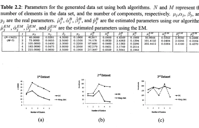
2.2 Parameters for the generated data set using both algorithms. N and M represent the number of elements in the data set, and the number of components, respectively.

ßj,aj, ßj, and pj are the real parameters, ßf, âf, ßf, and pf are the estimated

parameters using our algorithm. ßfM, âfM, ßfM, and pfM are the estimated

parameters using the EM 16

2.3 Bayesian and EM parameters estimation of the three dataseis using two

compo-nents GGM (B and EM denote Bayesian and EM estimations, respectively)

20

2.4 The Average (± standard deviation) classification accuracy, over 10 trials, of the

four different methods 23

2.5 Average Retrieval rate(%) for the four different methods 24 3.1 Summary of the results for the 100 generated data sets. M denotes the obtained

number of clusters 61

3.2 Parameters of four different generated data sets. N represents the number of

ele-ments in each data set. rrij, Sj, and pj are the real parameters, rhj, Sj, and pj are

the estimated parameters 61

3.3 Estimated posterior probabilities of the number of components given the data for the four data sets, with percentage of accepted Split-Combine, and Birth-Death

moves 63

3.4 Parameters of the mixture models representing the different tested real data sets.

j component number, rrij, Sj, and pj are the real parameters, rhj, Sj, and 1E are

the Beta mixture estimated parameters. ßj; s|, and p? are the Gaussian mixture

estimated parameters 65

List of Figures

2.1 Generalized Gaussian Distributions with different values of the shape parameter. .

8

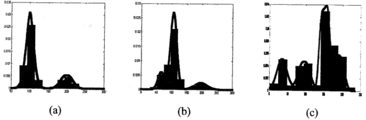
2.2 Real and estimated histograms for the three dataseis, (a) First dataset with M=2,

(b) Second dataset with M=3, (c) Third dataset with M=A 15

2.3 Marginal Likelihood and BIC values for the three dataseis with different number

of clusters, (a) First dataset, (b) Second dataset, (c) Third dataset

16

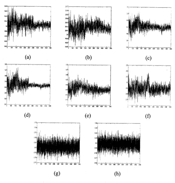
2.4 Time series plot of Gibbs-within-Metropolis iterations for the first dataset. (a)

Iterations for Ji1, (b) Iterations for µ2, (c) Iterations for a?, (d) Iterations for ä2, (e)

Iterations for Â,(f) Iterations for /32, (g) Iterations for j9!,(h) Iterations for p2. ... 17

2.5 Real and estimated histograms for the dataset using both algorithms (a) Bayesian

algorithm, (b) EM algorithm ig

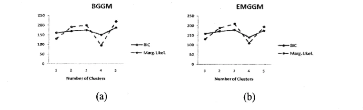
2.6 Marginal Likelihood and BIC values for the dataset with different number of

clus-ters using the two algorithms, (a) Bayesian algorithm, (b) EM algorithm

18

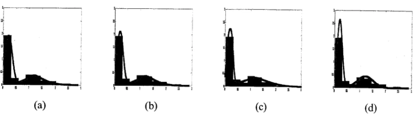
2.7 Real and estimated histograms for the enzyme data set. (a) Using Bayesian

esti-mation for GGM, (b) Using EM for GGM, (c) Using Bayesian estiesti-mation for GM,

(d) Using EM for GM 19

2.8 Real and estimated histograms for the acidity data set. (a) Using Bayesian

estima-tion for GGM, (b) Using EM for GGM, (c) Using Bayesian estimaestima-tion for GM, (d)

Using EM for GM 19

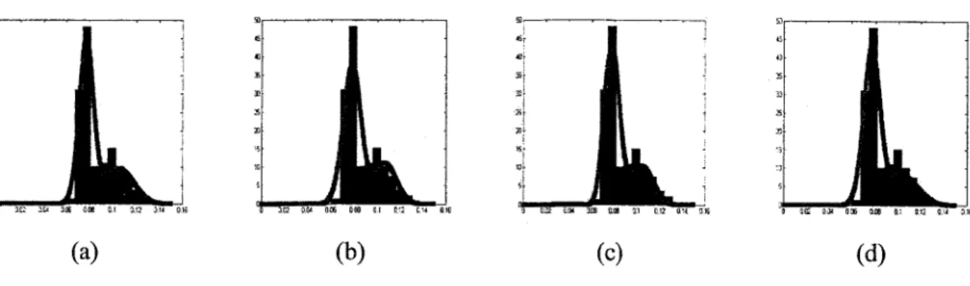
2.9 Real and estimated histograms for the stamp data set. (a) Using Bayesian

estima-tion for GGM, (b) Using EM for GGM, (c) Using Bayesian estimaestima-tion for GM, (d)

Using EM for GM 20

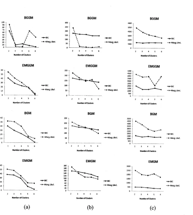
2. 10 BIC and Marginal Likelihood for several values ofMwhen using the four different

methods, (a) For the Enzyme dataset, (b) For the Acidity dataset, (c) For the Stamp

dataset 27

2.1 1 Original image and its steerable pyramid decomposition, (a) Original image from

Bark group in Vistex, (b) Sub-images output using five level steerable pyramid. . . 28

2.13 An example of the Sub-image real and estimated histogram using 5 components

GGM 28

2.14 Sample images from each group, (a) Bark, (b) Fabric, (c) Food, (d) Metal, (e)

Sand, (f) Water. 29

2.15 Average retrieval rate, (a) Precision rate using the 4 different methods for each of the 6 classes used, (b) Overall recall rate using the 4 different methods 29 2.16 Tested images (a) Complex PCB, (b) PCB with text, (c) PCB with noise, (d) PCB

with missing components 29

2.17 Segmentations results for Fig 2. 16. a. (a) Bayesian Generalized Gaussian Mixture, (b) E-M Generalized Gaussian Mixture, (c) Bayesian Gaussian Mixture, (d) E-M

Gaussian Mixture 30

2.18 Segmentations results for Fig. 2.16.b. (a) Bayesian Generalized Gaussian Mixture, (b) E-M Generalized Gaussian Mixture, (c) Bayesian Gaussian Mixture, (d) E-M

Gaussian Mixture 31

2.19 PCB Original image corrupted with noise (Fig 2.16.c) and its segmentations using the four methods, (a) Bayesian Generalized Gaussian Mixture, (b) E-M General-ized Gaussian Mixture, (c) Bayesian Gaussian Mixture, (d) E-M Gaussian Mixture. 32 2.20 Segmentations results for Fig 2.16.d. (a) Bayesian Generalized Gaussian Mixture,

(b) E-M Generalized Gaussian Mixture, (c) Bayesian Gaussian Mixture, (d) E-M

Gaussian Mixture 33

2.21 Tested SAR images (a) First image (Courtesy ofNASA), (b) Second Image (Cour-tesy of NASA), (c) SAR image (Cour(Cour-tesy of European Space Agency) 34 2.22 SAR image (Fig. 2.2 1 .a) and its segmentations using the four methods, (a) Bayesian

Generalize Gaussian Mixture, (b) E-M Generalize Gaussian Mixture, (c) Bayesian

Gaussian Mixture, (d) E-M Gaussian Mixture. 35

2.23 SAR image (Fig. 2.21 .b) and its segmentations using the four methods, (a) Bayesian Generalize Gaussian Mixture, (b) E-M Generalize Gaussian Mixture, (c) Bayesian

Gaussian Mixture, (d) E-M Gaussian Mixture. 36

2.24 SAR image (Fig. 2.2 1 .c) and its segmentations using the four methods(a) Bayesian Generalize Gaussian Mixture, (b) E-M Generalize Gaussian Mixture, (c) Bayesian

Gaussian Mixture, (d) E-M Gaussian Mixture 37

2.25 Microscopic images used, (a) The rat spleen tissue pulps (Courtesy of Dr. Jinglu Tan), (b) Lung Carcinoid tumor (Courtesy of Dr. Robert Cardiff) 39 2.26 The different stage outputs for the two methods on the rat spleen tissue, (a) The

gray scale image, (b) the image after histogram adjustment, (c) The identified ob-ject of interest using our method, (d) The identified obob-ject of interest using the

2.27 The different stage outputs for the two methods on the Lung Carcinoid tumor, (a) The gray scale image, (b) the image after histogram adjustment, (c) The identified object of interest using our method, (d) The identified object of interest using the

state of the art algorithm 41

2.28 Five noisy spots obtained from the 1230clG/Rmicroarray image 43 2.29 The Experiment results of the three methods on the five noisy spots 44 3.1 Graphical Model representation of the Bayesian Hierarchical finite general Beta

mixture model. Nodes in this graph represent random variables, rounded boxes are fixed hyperparameters, boxes indicate repetition (with the number of repetitions in the lower right) and arcs describe conditional dependencies between variables. . . 55 3.2 Real and estimated histograms for four generated data sets, (a) a 2 components

mixture, (b) a 3 components mixture, (c) a 4 components mixture, (d) a 5

compo-nents mixture 62

3.3 Enzyme data modeling when considering the mixtures with the highest probabili-ties, (a) Beta mixture models, (b) Gaussian mixture models 64 3.4 Acidity data modeling when considering the mixtures with the highest

probabili-ties, (a) Beta mixture models, (b) Gaussian mixture models. 65 3.5 Galaxy data modeling when considering the mixtures with the highest

probabili-ties, (a) Beta mixture models, (b) Gaussian mixture models 66 3.6 Stamp data modeling when considering the mixtures with the highest probabilities.

(a) Beta mixture models, (b) Gaussian mixture models 67

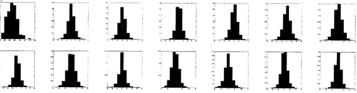
3.7 Original image and its steerable pyramid decomposition, (a) Original image from Bark group in Vistex, (b) Sub-images output using five level steerable pyramid. . . 67 3.8 Histograms of the 14 sub-images of the steerable pyramid 68

3.9 A sub-image histogram fitted by a Beta mixture model 68

3.10 Sample images from each group, (a) Bark, (b) Fabric, (c) Food, (d) Metal, (e)

Sand, (f) Water. 70

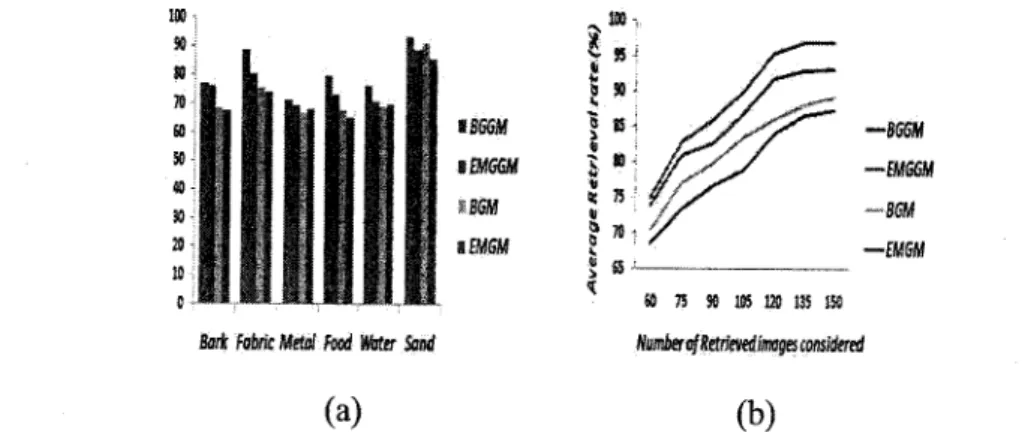
3.1 1 Precision and recall, (a) Average precision when 64 retrieved images are consid-ered for each class, (b) Average precision when varying the number of retrieved images, (c) Average recall when varying the number of retrieved images 71

Chapter 1

I

Introduction

Over the last decade, technological advances have led to an explosion of enormous data size. These data pose a challenge to standard statistical methods and have received much attention recently. The importance of finding a way to model and analyze data lie in their usefulness in wide range of applications such as Bioinformatics, image processing, and computer vision. In recent years a lot of different algorithms were developed in the aim of automatically learning to recognize complex patterns, and to make intelligent decisions based on observed data. Machine learning is a scientific discipline that is concerned with the design and development of algorithms that allow computers to change behavior based on data, such as from sensor data or databases. A major focus of machine learning research is to offer a principled approach for developing and studying automatic techniques capable of learning their parameters based on training data [1-4}. Machine learning and statistical pattern recognition have seen dramatic growth over the past few years, this is due to the fact that it can be applied in diverse areas such as engineering, medicine, computer science, psychology, neuroscience, physics, and mathematics. In many statistical applications the observed data can be seen as stemming from multiple populations. It is ofinterest to build a generic model, which allows us to combine the samples from different populations.

Mixture models are one of the machine learning techniques receiving considerable attention in different applications. They are an interesting and flexible model family. The different uses of mixture models include for example clustering and density estimation. Moreover, mixture models

have been successfully used in various kinds of tasks such as modeling failure rate data, and

clus-tering teaching behavior. Although mixture models have been applied in different areas, they have

proven particular efficiency in quality control systems.

In telephone networks, for instance, mixture models were applied in order to evaluate and

monitor speech quality [5]. For software quality prediction, mixture models are used as a tool for

early prediction of fault-prone program modules [6, 7]. In Bioinformatics, the analysis of DNA

microarray data sets can be important in order to diagnose and discover different types ofdiseases,

the use ofmixture models can lead to a better treatment ofpatients in high risk [8]. Mixture models

can be finite or infinite [9, 10]. In this thesis, we are only interested in finite mixture models.

1.1

Finite Mixture models

Finite mixture models assume that each component comes from a probability distribution, P,

which has a given weight pjt j = 1,...,M7 where the sum of the weights of all components is

equal to one and M represents the total number of components. Finite mixture models can be

represented by

M

?(?\T) = S?,?(?\??)

(1)

where p¡ (0 < p3 < 1 and Y,f=lPj = 1) are the mixing proportions and P(X]Qj), is the

prob-ability density function describing component j. The symbol Sj, j = 1,...,M, represents the

different parameters vectors of the mixture components. In order to use mixture models, three

main problems have to be resolved: the choice of the probability density function (PDF),

parame-ters estimation and the selection of the number of clusparame-ters.

1.1.1 Probability Density Function Selection

The selection of the PDF to be used for modeling the data is of a crucial importance, because

it affects the capability of the mixture to represent the data shape. The wrong selection of PDF

may force the mixture model to increase the number of components in order to model the data (i.e overfitting). In most of the applications, the Gaussian density is used in the mixture modeling of data. As a smooth, bell-shaped distribution that can be completely characterized by its mean and its standard deviation, the Gaussian is in general used and justified for asymptotic reasons (i.e the sample is supposed to be sufficiently large) [H]. Although a Gaussian mixture may provide a reasonable approximation to many real-world distributions, it is certainly not always the best approximation especially in image and signal processing applications where we often deal with small samples [12-15]. Indeed, there are many phenomena and applications for which the Gaus-sian model is not realistic (for instance, it is well-known that natural image clutter is generally non-Gaussian). In this thesis, we consider the generalized Gaussian distribution (GGD) and the general Beta distribution as they can be good alternatives to the Gaussian distribution thanks to their shape flexibility which allows the modeling of a large number of non-Gaussian signals [12, 16-19].

1.1.2

Parameters Learning

Parameter learning approaches are used in order to estimate the model parameters. This problem is not straightforward and many deterministic as well as Bayesian approaches have been proposed. In deterministic approaches, parameters are assumed as fixed and unknown, and inference is founded on the likelihood of the data. Despite the fact that deterministic approaches have dominated mix-ture models estimation due to their small computational time, many works have demonstrated that these methods have severe problems such as convergence to local maxima and their tendency to overfitt the data [11], especially, when data are sparse or noisy. With the computational tools evo-lution, researchers were encouraged to implement and use Bayesian Markov Chain Monte Carlo (MCMC) methods and techniques as an alternative approach [20, 21]. Bayesian methods consider parameters to be random, and to follow different prior distributions. These distributions are used to describe our knowledge before considering the data, as for updating our prior beliefs the likelihood is used. Please refer to [1 1, 22] for interesting and in depth discussions about the general Bayesian

theory. In this thesis, we are interested in the application of MCMC methods for the estimation of the model parameters.

1.1.3

Selection of the number of components

An important issue in mixture modeling is the selection of the number of components. The usual

tradeoff in model order selection problems arises: with too many components, the mixture may

overfitt the data, while a mixture with too few components may not be flexible enough to

approxi-mate the true underlying model. Lack of knowledge about the number of clusters is a challenging

problem in mixture modeling and considerable efforts already have been made to investigate this

important aspect. The majority of the approaches that have been proposed separate the estimation

and the selection of the number of components (i.e a certain criterion should be compared for

dif-ferent number of clusters) (see, for instance, [9, 10] for interesting discussions and comparisons

between different criteria). In this thesis, we use two different methods in order to select the

num-ber of clusters. The first method, is used to compare different values of M and finally select the

one that increases the marginal likelihood ofthe data. For this method, we employ two criteria: the

Bayesian information criterion (BIC) and the Laplace approximation. The other method takes into

account the fact that both estimation and selection problems are strongly related. In order to apply

this method we are using the Reversible Jump MCMC (RJMCMC) to simultaneously estimate and

select mixture models parameters.

1.2 Contributions

The contributions of this thesis are as follows:

<&- A Bayesian Approach for Finite Generalized Gaussian Mixture Models Learning:

We implement a fully Bayesian approach to analyze GGM models. Our approach evaluates the

selection uses the integrated likelihood. We then validate this novel approach by applying it to different image processing applications; while comparing it to different other approaches.

<®° A Fully Bayesian Model Based on RJMCMC and Finite Beta Mixture:

We propose a Bayesian model founded on the RJMCMC for the General Beta distribution. Our ap-proach is able to select and estimate finite Beta mixture models simultaneously. This was reached by treating the number ofclusters as a random variable having a prior distribution. We then demon-strate its effectiveness using synthetic mixture data, real data, and image texture classification and

retrieval.

1.3 Thesis Overview

The organization of this thesis is as follows:

D The first Chapter contains an introduction to finite mixture models.

Q In Chapter 2, we introduce a Bayesian model based on Gibbs sampling, integrated likelihood, and finite Generalized Gaussian mixture. We investigate the effectiveness of our model by comparing it to different Bayesian and deterministic methods in various image processing applications.

Q In Chapter 3, we propose a fully Bayesian algorithm for Beta mixtures learning based on the RJMCMC technique. We study the capability of our model in texture classification and retrieval while comparing it to the Gaussian mixture model.

Chapter

2

Bayesian Learning of Finite Generalized

Gaussian Mixture Models on Images

This chapter presents a fully Bayesian approach to analyze finite Generalized Gaussian mixture

models which incorporate several standard mixtures, widely used in signal and image processing

applications, such as Laplace and Gaussian. Our work is motivated by the fact that the Generalized

Gaussian Distribution (GGD) can be applied on a wide range of data due to its shape

flexibil-ity which justifies its usefulness to model the statistical behavior of multimedia signals [23]. We

present a method to evaluate the posterior distribution and Bayes estimators using a Gibbs

sam-pling algorithm. For the selection of number of components in the mixture, we use the Laplace

approximation and Bayesian information criterion. We validate the proposed method by applying

it to: synthetic data, real dataseis, texture classification and retrieval, and image segmentation;

while comparing it to different other approaches.

2.1 Introduction

Finite mixtures are a flexible and powerful probabilistic tool for modeling data [9]. Mixture

mod-els are very useful in areas where statistical modeling of data is needed such as in signal and image

earlier, the three main problems in mixture modeling are the choice ofthe probability density

func-tion (PDF), the parameters and model learning. Many studies have shown that the GGD, can be a good alternative to the Gaussian thanks to its shape flexibility which allows the modeling of a large number of non-Gaussian signals [12, 16-18]. The GGD contains the Laplacian, the Gaussian and asymptotically the uniform distribution as special cases [24] and has been used, for instance, in [14,25] to fit subband histograms, in [26] for multiresolution transmission of high-definition video, in [27] for subband decomposition of video, in [28] for buffer control, in [29-31] for

tex-ture classification and retrieval, in [32] for denoising applications, in [33, 34] for data and image

compression, in [35] for edge modeling, in [36,37] for image thresholding, in [38, 39] for speech

modeling, in [40, 41] for video and image segmentation, in [42] for SAR images statistics model-ing, and in [43] for multichannel audio resynthesis.

Several approaches have been considered in the past to estimate GGD 's parameters such as mo-ment estimation [27,44,45], entropy matching estimation [39,46], and maximum likelihood

es-timation [12,29,44,47,48]. It is noteworthy that these approaches consider a single distribution.

Concerning finite mixture models parameters estimation, some deterministic approaches have been

proposed in the past for the estimation of finite generalized Gaussian mixture (GGM) models

pa-rameters (see, for instance, [40,41]). To the best of our knowledge the learning techniques that

have been proposed for the GGM are deterministic and then usually excessively sensitive to noise.

Thus, we propose in this chapter a novel Bayesian approach to evaluate the posterior distribution of

GGM and then learn its parameters using Gibbs sampling [49] for the estimation and the integrated

likelihood for the selection of the optimal number of components. To validate our learning

algo-rithm, we compare it to three different techniques: the expectation-maximization (EM) estimation

of the GGM, the EM and Bayesian approaches for the Gaussian mixture (GM) using synthetic

data, real dataseis, and real world applications involving texture classification and retrieval, image

2.2

The Finite GGM and Bayesian Estimation

2.2.1 Finite GGM Model

Ifthe random variable ? e E follows a GGD with parameters µ, a and ß, then the density function

is given by [25,27]:

0a ,_.,_ ..,xa

(1)

?{?\µ,a,ß) = „J!i*,Me-Wx-rtß

_2G(1//3)

where a = ?^/?|?|1, -?? < µ < ??, /? > 0, and a > 0, and G(.) is the Gamma function given

by: T(x) = f™ t^e^dt, ? > 0. µ, a and /? denote the distribution mean, the inverse scale

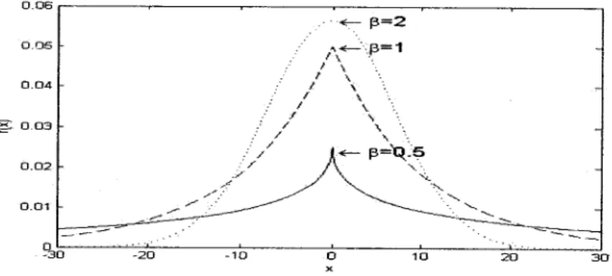
parameter, and the shape parameter, respectively. The parameter ß controls the shape of the pdf.

The larger the value, the flatter the pdf; and the smaller the value, the more picked the pdf. This

means that ß determines the decay rate of the density function (see Fig. 2.1). Note that for the

Ä- O 03

(-P=R-S

Figure 2.1: Generalized Gaussian Distributions with different values of the shape parameter.

two special cases, when ß = 2 and ß - 1, the GGD is reduced to the Gaussian and Laplacian

distributions, respectively. If ? follows a mixture of M GGDs, then

M

where Pj (O < Pj < 1 and ]T\=1 pj = 1) are the mixing proportions andp(x|^, O7-, /?,·) is the GGD

describing component j. As for the symbol ? = (?, ?), it refers to the entire set of parameters to

be estimated, knowing that ? = (µ?, «?, ß?, ..., µ?, a?, Pm), and ? = (ph ...,??).

Consider N observations, X = (X1, ..., xN), the well-known approach to estimate the parameters

of a mixture model is to maximize the likelihood through the expectation-maximization (EM)

algorithm [50], supposing that the number of mixture components M is known. The likelihood corresponding to this case is:

N M

?(*??) = ?S*<?*&)??

(3>

¿=1 j=l

Where ?^ = (ß^a^ßj). For each variable x¿, let Zi be an M-dimensional vector known by the

unobserved or missing vector that indicates to which component x¿ belongs, such that: Zi3- will be

equal 1 if x¿ belongs to class j or O, otherwise. The complete-data likelihood is then:

N M

p(X,Z\e) = lHl(p(xt\QPj)zv

(4)

z=l j=l

Where Z = {Zi,Z2,...,ZN}. The EM algorithm consists of getting the mixture parameters that

maximize the log-likelihood function given by:

M N

L(G, ?,?) = SS zv log(P(*ifo>¿)

(5)

j = l 2 = 1

by replacing each Z^ by its expectation, defined as the posterior probability that the ith observation arises from the jth component of the mixture as follows:

Zw = y v *ISj ,yi {¿\

where í denotes the current iteration step and £J4) and pf* are the current evaluations ofthe

param-eters. The EM produces a sequence of estimates to the mixture parameters T*, for t = 0, 1, . . .,

until a certain convergence criterion is satisfied through two different steps: the expectation and

1 . Initialization of the mixture paraneters.

2. ?-step: Compute Z^ (Eq. 6) using the initialized parameters.

3. M-step: Update parameters estimates using: ?(?) = argmaxe ¿(??_1, Z, X)

However, the EM has some drawbacks, like convergence to local maxima due to its dependence on the initialization step. For a detailed and interesting discussion about EM disadvantages please refer to [50]. An efficient alternative technique that we will propose in the following is the Bayesian approach which has received a lot of attention recently thanks to the evolution of Markov Chain Monte Carlo (MCMC) computational tools.

2.2.2

Bayesian Estimation of the GGM

Simulation methods like MCMC algorithms are chosen as a solution to overcome the problems of numerical methods. Generally these methods are related to the Bayesian theory, which means that they allow for probability statements to be made directly about the unknown parameters of the mixture, while taking into consideration prior or expert opinion. The goal is to get the posterior

distribution p{ß\?,?), by combining the prior information about the parameters, p(?), with

the observed value or realization of the complete data p(X, ?\T), which is derived from Bayes

formula:

Where (X, Z), is the complete data. Having the joint distribution, p(?)?(?, ?\?), we can deduce

the posterior distribution (Eq. 7). With p(?\?, Z) in hand we can simulate our model parameters

T, rather than computing them. The Gibbs sampler is a well known simulation technique [49]

and it is based on the successive simulation of Z, p, and ? conditional on each other and on the observations which offers an efficient way to explore the parameter space. The standard Gibbs sampler for mixture models consists of:

2. Stepí, fori = 1,...

(a) Generate ?® from tt(?|T, X).

(b) Generate ?® from p(?|?^).

(c) Generate ?« from tt(£|?« , X).

We simulate Z according to the posterior probability p(?\?,?), chosen to be Multinomial of order one with a weight given by Zi0[M[I; Zn;...; ZiMj). This choice is due to two reasons, first,

we know that each Z¿ is a vector of zero-one indicator variables to define from which component

j the ? observation arises. Second, the probability that the ith observation, xi} arises from the jth

component of the mixture is given by Z^. So, we can deduce that each vector Zi is generated by

a Multinomial distribution of order one with weight given by Zy. Now to simulate ? we need to

get p(?\?®), using Bayes rule: p[?\?) = f^tít) ? p(?\?)p(?)· This means that we need to

determine p[?\?), and p(?). It is well known that the vector ? is defined as (^rLi Pj = 1> where

Pj > 0), then the commonly considered choice as a prior is the Dirichlet distribution [1 1, 22]:

nip)=w^)Up'

(8)

Where (^1, . . . , ??) is the parameter vector ofthe Dirichlet distribution. As for p(?\?) we have:

M NM M

p[?\?) = J] ,T(ZiIp) = ¡J IK" = Up?

(9)

j=l i=l j=l J-=I

Where Ti7- = X)i=rl Izij=1 , then we can conclude that:

p(?|?) = Tr(ZIP)TT(P) = ^%) , ?^G*'"1 a P^ + »?· -> ^ + "") (10>

_{Hj=I -t TOJ j=l}

where V denotes the Dirichlet distribution with parameters [?? + ??,...,?? + nM). Thus, we can

deduce that the Dirichlet distribution is a conjugate prior for the mixture proportions (i.e the prior

and the posterior have the same form). As for the parameters ?, we assigned independent Normal

priors for the distributions means, and Gamma priors for the inverse scale and shape

parame-ters [5 1, 52]: ßj ~ ?G(µ0, ajj) , ßj ~ Q(ocp, ßß) , a¿ ~ G(aa, ßa), where ??(µ0, s%) is the normal

distribution with mean µ0 and variance s\, Gi&ß, ßß) is the gamma distribution with shape

param-eter aß and rate paramparam-eter ßß. µ0, s$, aß, ßß, aa, ßa are called the hyperparamparam-eters of the model.

Having these priors in hand, the posterior distributions for µ, a, and ß are (see Appendix A): (Mi-Mo)2 . ^ ? ? |\|8,·

p(µ^?, X) oc e 2s? '-7-1 (H)

n(aj \Z, X) oc a?ß"V^ (a,·)^ßS^=? (-^-^'1^'

(12)

t?(^??,?') oc ßC^e-Wii-Jti—?^??^{-a^'?[?3

(13)

In this case we can notice that our posterior distributions are not in well known forms, so we cannot simulate directly from these posterior distributions. The Metropolis-Hastings (M-H) algorithm [51] offers a solution for this problem, and thus the complete algorithm is given by:

1. Initialization: choose p0 andG0 2. Stepi, fori = 1,...

(a) Generate zf ~ (M(I; Zn; ...; ZiM))

(b) Compute nf = J2?=1 1 <t)

(c) Generate pW fromEq.(lO).

(d) Generate (µ,-, qj, ß)<*> for (j = 1, ..., M) from Eqs.( 1 1), ( 12), and( 13) using M-H

algorithm.

The M-H algorithm can be summarized in 3 steps:

1. Generate (fi^a^ßy) ~ q(ßj,aj,ßj \ µ^ , af~1] , ß^*~?)) andU ~ W[0,i]

2 rnmtiiitc r -

F^?^?^?'^G1^-5^)

3. Ifr < U then {µ?, af, ßf) = (µ,, a,, ß) else (µ«, af, ß?) = (µ™ ,a™, ß™)

The major problem in this algorithm is the need to choose the proposal distribution q. To solve

this problem we used the most generic random walk M-H by considering the following proposals:

S5 ~ Ctf{\og{p%-\ C2), ßj ~ £7\A(log(/f"x)), C2), where CM is the log-normal distribution,

since, we know that Sj > O and ßj > O. As for fi¡¡ we have µ3 ~ ?(µ^~1\ ?2), where C2 is the

scale of the random walk. With these proposals the random walk M-H algorithm is composed of

the following steps:

1. Generate µ3 ~ M(^, ?2), Sj ~ CM^af'^^2), 03 ~ CM(log(ßf^), ?2), and

U ~ W[o,i] 2. Compute

?µ <ß{r]\Z^)M{ßj\^~l\c2)

r

Ir(Sj]Z, X)CN(a{;-l) J logfc·), C2)

iriaf-» I Z, X)CM[S3 1 ?f$-\ ?2)

r

p(^[?, ?-)£?G(^-1}[ IQg(^), C2)

Tß n(ß^\Z,X)CM(ß3\\og(ßf-\(*)

3.

. If?µ > u then ¿if = µ3, else /if = µ^

• Ifra > u then af = a,·, else af = ajt_1)

• If?, > u then /?f = ßj, else /?f = ßf~x)

2.3

Experimental results

2.3.1 Design of Experiments

In this section, we apply our Bayesian GGM estimation algorithm for synthetic data, real dataseis,

and real applications involving texture classification and retrieval, and image segmentation. We

(14) (15) (16)

validate our algorithm by comparing it to the EM approach, the EM and Bayesian approaches for the well-known GM. In fact, choosing a relevant model consists both of choosing its form (GGM or GM in our case) and the number of components M. We use two approaches in order to rate the ability of the tested models to fit the data or to determine the number of clusters M. The first criterion is one of the key quantities used for Bayesian hypothesis testing and model selection, the integrated or marginal likelihood defined by [53]:

p(X\M) = I p(?\?, M)dQ = ??(?\?, ?)p(?\?)??

(17)

where ? is the vector of parameters of a finite mixture model, p(?\?) is its prior density, and

?(?\?, M) is the likelihood function taking into account that the number of clusters is M. Using

the Laplace approximation as in [53] we get:

- ^N 1 ~

log(p(X\M)) « log(p(X\e, M)) + log(7r(9|M)) + -f 1?§(2tt) + - \og{\H{Q)\)

(18)

where \H(Q)\ is the determinant of the Hessian matrix, and Np is the number of parameters to

be estimated which is equal to (4M) for the GGM. We can use the Laplace-Metropolis estima-tor [53] which consist of finding the Metropolis estimates of ? and ?(?). With samples of the

posterior parameters simulated from the M-H in hand, we estimate ? as the ? in the sample at

which the likelihood ?(?\?, M) achieves its maximum. For the other quantity needed ?(?) it

is asymptotically equal to the posterior covariance matrix, and could be estimated by the sample

covariance matrix of the posterior simulation outputs. The second approach is the Bayesian

In-formation Criterion (BIC) of Schwartz [54] which is actually an approximation for the integrated

likelihood criterion [53]: BIC = log(X\M,§M) - ^log(N). In the following applications,

we have used 5000 iteration for our Metropolis-within-Gibbs sampler (we discarded the first 800 iterations as "burn-in" and kept the rest), and our specific choices for the hypeparameters are (µ0, s?, aa, ßa, aß, ßß) = (0,1, 0.2, 2, 0.2, 2). As for the scale of the random walk we use it as

Table 2.1: Parameters for the different generated data sets. N represents the number of elements

in each data set. µ?,a^ ß?, and p¿ are the real parameters. µ?, âjt fy, and pó are the estimated

parameters. Data 1 (JV=262144) Dala 2 (^=65536) Data 3 (?=97344) 100.0000 200.0000 63.6283 104.68S4 195.2122 33.1256 95.5550 150.5876 185.9900 0.0778 0.0406 0.0700 0.0603 0.0333 0.0500 0.0450 0.0650 0.0400 1.7000 2.3000 2.1000 1.9000 1.7000 2.0000 2.4000 3.5000 3.1000 0.7800 0.2200 0.1458 0.7370 0.1172 0.1721 0.2000 0.3700 0.2579 100.0086 200.0248 65.1100 106.0010 196.5765 33.7487 95.7038 150.0495 185.3104 0.0704 0.0434 0.0692 0.0658 0.0340 0.0509 0.0434 0.0636 0.0409 1.7300 2.2900 2.0000 1.9400 1.6600 1.9899 2.4368 3.7778 3.1177 0.7799 0.2201 0.1523 0.7222 0.1255 0.1768 0.1928 0.3751 0.2552

2.3.2

Synthetic Data

This section has two main goals, first testing the effectiveness of the algorithm to: estimate the

mixture parameters and to select the number of clusters. Then to illustrate the higher performance

ofour algorithm compared to the EM estimation. To reach our first goal we generated three dataseis

and applied our method to estimate the parameters and select the number of components of the

associated mixture models. Table 2.1 contains the real and estimated parameters of the generated

dataseis. Fig. 2.2 shows the real and the estimated histograms of the three generated data sets.

The integrated likelihood and the BIC calculated for different number of clusters (M=I, 2, 3, 4

and 5) of the above datasets are given in Fig. 2.3. Fig. 2.4 shows the time series plot of our

2B 260 303

(a) (b) _(e)

Figure 2.2: Real and estimated histograms for the three datasets. (a) First dataset with M=I, (b)

Table 2.2: Parameters for

number of elements in thethe generated data set using both algorithms. N and M represent the

_{data set, and the number of components, respectively, µ,-,a^·, /3,·, and}

Pj are the real parameters. fif,af, ßf, and pf are the estimated parameters using our algorithm.

f-EM ?EM

_{ßfM, and pfM are the estimated parameters using the EM.}

"HT v-i ßi Pi ßf ??_ 4*-'M ß:?,?? r-j (/V- 15625) (?/=5) 40.0000 75.0000 105.0000 182.0000 215.0000 0.0381 0.0655 0.0400 0.0475 0.0600 4.5000 2.5000 3.3000 3.0000 3.5000 0.1900 0.1500 0.2200 0.2500 0.1900 40.2617 74.1178 107.6681 182.2170 217.3647 0.0400 0.0620 0.0460 0.0451 0.0559 4.4549 2.4363 3.1363 3.1749 3.5041 0.1889 0.1394 0.2286 0.2514 0.1963 50.8644 101.4133 202.4412 0.0343 0.0404 0.0364 2.8050 2.0245 2.4100 0.2466 0.3164 0.4370 1* Dataset -«-Mafg.táeL Numberof Clusters (a) 2nd Dataset

Number oí eluden

(b)

3rd Dataset

12 3 4

Number cföusiers

(e)

Figure 2.3: Marginal Likelihood and BIC values for the three dataseis with different number of clusters, (a) First dataset, (b) Second dataset, (c) Third dataset.

Bayesian algorithm iterations by taking the first dataset as an example. We can see clearly that our algorithm is able to get the exact number of clusters and a very good approximation of the mixtures parameters of the generated data sets. For the second goal, we generated a dataset that

has five components and applied both methods (Bayesian and EM) to check ifthey can approximate

it effectively. For our algorithm, it was able to: recognize that the dataset is generated from five classes, and to estimate its parameters effectively. As for the EM algorithm its selection of the number of components was wrong which forces it to a false estimation of the parameters. Table 2.2 contains the real and estimated parameters of the generated dataset using both algorithms. Fig. 2.5 shows the real and the estimated histograms of the dataset using the two methods. The

¦3 -m ¡ss «a? za¡ ¡ss m ?mìw ¿sa

aœ-(a)

" 3 MC ISX -535 3* SC MC XX- JJK " O 5X

(F

U3 KK íSM KS S» m 3S» «03 «B SBO IC-X E-K 3K6 2KS 3-K -sa ߣ ;ac- »ï

(b) (e)

:z ¡oe rar; 2:0c ss ss »» ¿s» «? fît !¦>>; ?™ 3£C SOO

(e) (f)

5« us a aan ¡a a? m ; «ß o* yjt: 5KD :o¡ ?a;, $» ¿? ¿^

(g) (h)

Figure 2.4: Time series plot of Gibbs-within-Metropolis iterations for the first dataset. (a)

Itera-tions for µ?, (b) IteraItera-tions for µ2, (c) IteraItera-tions for O1, (d) IteraItera-tions for â2, (e) IteraItera-tions for Â, (f)

Iterations for /32, (g) Iterations for P1 ,(h) Iterations for ^2.

? a a a a m

(a) (b)

Figure 2.5: Real and estimated histograms for the dataset using both algorithms (a) Bayesian algorithm, (b) EM algorithm. BGGM 150 100 12 3 4 Number of Clusters (a) EMGGM -SiC - Wtarg, Ufceï, Z5ü 200 150 1OO 12 3 4 Number of Clusters (b) — *¦— Ma^g.lifeei,

Figure 2.6: Marginal Likelihood and BIC values for the dataset with different number of clusters using the two algorithms, (a) Bayesian algorithm, (b) EM algorithm.

2.3.3 Real Datasets

We devote this section to real datasets. Our method is used to model three standard widely used

datasets. The first one describes an enzymatic activity in the blood among a group of 245 unrelated

individuals, and the second one is an acidity index measured in a sample of 155 lakes in the

Northeastern United States. The third and last one, consists of thickness of 485 postage stamps

produced in Mexico. For these three data sets, a mixture of 2 distributions is generally identified

[55]. Figures 2.7, 2.8, and 2.9 show the real and the estimated histograms for the three datasets, respectively, when applying the GGM and the GM using EM and Bayesian approaches. In all

'J ¦ ' ' ! 'I ¦ ¦ : I - ¦ L , __

L^_ Lj L^ L^

(a) (b) (e) _(F

Figure 2.7: Real and estimated histograms for the enzyme data set. (a) Using Bayesian estimation

for GGM, (b) Using EM for GGM, (c) Using Bayesian estimation for GM, (d) Using EM for GM.

3S t 45 S 55

(a) (b) (e) (d)

Figure 2.8: Real and estimated histograms for the acidity data set. (a) Using Bayesian estimation

for GGM, (b) Using EM for GGM, (c) Using Bayesian estimation for GM, (d) Using EM for GM.

cases, it's clear that the GGM and the GM fit the data. The final results of the Bayesian and

EM estimations, in the GGM case, are given in table 2.3. The values of the BIC, and marginal

likelihood criteria for both GGM and GM using Bayesian and EM methods for different values of

M are given in Fig. 2.10. According to these figures the optimal number of components to fit the

three datasets in all cases is M = 2.

3C Iti 3Œ OJA ?.? c µ ß?e DEE OA OX 9JS el: ?.?;

(a) (b) (e) (d)

Figure 2.9: Real and estimated histograms for the stamp data set. (a) Using Bayesian estimation for GGM, (b) Using EM for GGM, (c) Using Bayesian estimation for GM, (d) Using EM for GM.

[ht!]

Table 2.3: Bayesian and EM parameters estimation of the three datasets using two components

GGM (B and EM denote Bayesian and EM estimations, respectively).

Enzyme Mode I Enzyme Mode 2 Acidity Mode 1 Acidity Mode 2 Stamp Mode i Stamp Mode 2 0.6325 0.1981 0.3675 1.2395 5.0556 2.0059 2.345 0.6040 0.1899 1.3347 0.3960 1.3119 6.0323 2.1682 0.5956 4.4279 0.4044 6.1410 1.8592 1.9923 2.2566 0.5998 1.0495 0.4002 4.3203 6.2820 2.2629 1.6287 1.8949 1.466« 1.9693 1.9987 0.7134 0.0774 101.4945 2.4315 0.6948 0.0773 95.0483 2.0311 0.2866 0.1025 65.7201 2.2048 0.3056 0.1066 65.0550 2.1729

2.3.4 Classification and Retrieval of Texture Images

Approach

Texture is one ofthe main characteristics used to describe natural images, which explain its impor-tant role in image processing, computer vision and pattern recognition applications. Texture analy-sis is a fundamental step in a variety of image processing applications such as industrial inspection, medical imaging, remote sensing, and content-based image classification and retrieval [29, 56, 57]. Texture analysis approaches can be divided into four categories: statistical, geometrical, model-based, and signal processing methods [58]. Many classification methods based on images fre-quency analysis have been proposed in the past. The basic assumption of these methods is that tex-ture can be identified by the energy distribution in the frequency domain via the decomposition of

the frequency spectrum into a sufficient number of sub-bands. Then, the statistics ofthe sub-bands

coefficients can be derived and modeled to distinguish different image textures. Indeed, texture

information can be modeled using second or higher order statistics [59] and it is well-known that

natural image textures generally give rise to non-Gaussian highly-peaked sub-bands densities [60].

In this section we propose an approach for texture images classification and retrieval based on

our GGM Bayesian learning algorithm. The used classification methodology, previously adopted

in [61] using GM, takes into consideration that signatures of different textures will differ when

transformed to frequency domain.

In our classification framework, an image texture is first transformed to gray scale and decomposed

into sub-bands using steerable filters [62, 63]. Figure 2.1 1 shows a texture image and its multiscale

version in a pyramid hierarchy. The histograms ofthe resulted filtered images are show in Fig. 2. 12

which shows clearly that the Gaussian assumption would be inappropriate. Then, each sub-band's

marginal density is approximated by a GGM model using our Bayesian estimation algorithm (see

Fig. 2.13). Finally, the Earth Mover's Distance (EMD) [64] is used to measure the distribution

similarity between a set of components representing an input image texture (ie. test image) and sets

of components representing texture classes (i.e training images). In our case, EMD can be viewed

as the minimum cost of changing one mixture into another, when the cost of moving probability

mass from components in the first mixture to components in the second mixture is calculated using

Kullback-Leibler (KL) divergence given by:

mU)= /Vi(Z)IOg(^)

(19)

Where /¿ is the component i of the input sub-image mixture, gó is the component j of the class

sub-image mixture. The derivation for the KL divergence ofthe Generalized Gaussian distribution

is known to be [29]:

Where (cti, /?¿) are the parameters of /¿, and (aij,ßj) are the parameters of ^. With KL in hand

we have to start the minimization problem in which we need to get the m ? ? matrix F, where /¿J is the amount of weight wxi matched to wyj (wxi and wyj are the weights of the distribution), that will minimize the following equation

m ?

EMDsub = S S f*DUi\\9i)

(21)

¿=i i=l

and subjected to the following constraints:(l) /^ > 0, where 1 < i < m and 1 < j < n, (2)

S™ ? fa = ^wi» where 1<3 <n> (3) EJ=i /y = wxi, where 1 < i < m, (4) X)^1 E"=i k =

min(wx, Wy), where wx = $^¿=i ""7^" an(^ ^y = S^=? w3/i· Note that when the image texture is

decomposed of L sub-bands, then the total EMD is the sum of that of each sub-band, EMD =

Sa=1 EMD5Uh1. By computing the EMD between the input texture image and each texture class,

each image is affected by the class for which the EMD is the smallest.

Results

The images that we have used in our experiments are from the MIT VisTex database ' . Six homo-geneous texture groups (Bark, Fabric, Food, Metal, Water, and Sand) were considered (Fig. 2.14). For each of the Bark, Fabric, and Metal texture groups, we used four 512 ? 512 images each di-vided into sixty four 64 ? 64 subimages. And for the Food, Water, and Sand texture groups, we used six 512 ? 512 images each divided into sixty four 64 ? 64 subimages as well. This gives us a total of 256 subimages for each class in the first three groups, and 384 subimages for each class in the second three groups. We then applied our classification approach 10 times, each time using 24 subimages of each original texture image for training and the remaining 40 for testing. This brings us to a total of 720 images from all six groups as training samples for our algorithm, and 1200 as testing samples. We compared the accuracy of our algorithm to classify all 1200 images to those of the three other methods (EM+GGM, Bayesian+GM, EM+GM). We applied our algorithm twice

Table 2.4: The Average (± standard deviation) classification accuracy, over 10 trials, of the four

different methods

______________Method Using 3 levels pyramid Using 5 levels pyramid Bayesian General Gaussian Mixture Models 94.12% ± 1.62% 95.62% ± 1.34%

EM General Gaussian Mixture Models 92.58% ± 1.74% 93.66% __ 1.69% Bayesian Gaussian Mixture Models 91.92% ± 1.36% 92.35% ± 1.51% ______EM Gaussian Mixture Models 90.83% ± 1 .92% 91 .97%) ± 2.72%

first using three levels pyramid and second using five levels pyramid to compare the two cases

together (see Table 2.4). From these results we can observe two main points: our algorithm has the

highest accuracy and as expected the five levels pyramid improves the performance over the three

levels pyramids, however this improvement is very small compared to the enormous difference in

computational time.

In the retrieval application, we have used each and every subimage as a query and checked ifwe

are able to retrieve all the other 64 subimages coming from the same mother image. Our retrieval

approach can be divided into two steps. First task, is the same as the classification approach, we

classify the image into one ofthe six groups. For the second step, we compare the input image with

the other images in the same group and retrieve the closest images to our query. We applied our

retrieval process twice former using three levels pyramid and latter using five levels pyramid. To

measure the retrieval rates (precision and recall), each image was used as a query and the number

of relevant images among those that were retrieved was noted. Table 2.5 presents the retrieval

rates obtained in terms ofprecision when 64 images are retrieved each time in response to a query.

Note that in this case the precision and recall are the same because for a given image we have

at most 64 images which are similar to it. Figure 2.15(a) displays the average (averaged over all

the queries) precision rate for different texture classes when we consider only the first 64 images

retrieved. Figure 2.15(b) shows two graphs the overall recall of our retrieval method when varying

the total number of images retrieved taken into consideration. According to the results in Table 2.5

[ht!]

________Table 2.5: Average Retrieval rate(%) for the four different methods

Method Using 3 levels pyramid Using 5 levels pyramid

Bayesian General Gaussian Mixture Models 81.25% 83.81%

EM General Gaussian Mixture Models 76.37% 79. 1 6%

Bayesian Gaussian Mixture Models 72.91% 74.52%

EM Gaussian Mixture Models 7 1 .66% 72. 1 2%

method. Second, it is enough to use three levels pyramid due to the large computational difference between it and the five levels pyramid, and the small difference in their effectiveness.

2.3.5

Image Segmentation

Image segmentation is one of the most significant problems, due to the fact that it is fundamental to many tasks of pattern recognition, image processing, computer vision where the segmentation

results generally govern the final quality of interpretation. Several approaches have been proposed

in the past. Many techniques, based on finite mixture Gaussians, have been developed, also, where

the idea was to partition the image in regions (each associated with one mixture component).

However, generally the pixel intensities inside the image regions are heavy-tailed which force the Gaussian mixture model to lose its accuracy. Often, image segmentation must be done in an unsupervised fashion in that training data is not available and the class conditioned feature vectors

must be estimated directly from the data. In this section, we apply our estimation algorithm for the

segmentation problem by formulating it as a classification problem with mixtures of generalized

Gaussian distributions. It is noteworthy to mention that the main purpose of this application is

to compare our Bayesian estimation with the EM one and with the results obtained when using

Gaussian mixture models. Comparisons with the several other segmentations approaches that have

been proposed in the past is out of the scope of our work.

We tested the effectiveness of our method on two different types of images, Printed circuit

board (PCB) and Synthetic Aperture Radar (SAR) images, we decided to use these images because

of their non-Gaussian characteristics.We began our experiment by applying our algorithm on four

complex electronic printed circuit board (PCB) images, to check if the algorithm is able to

rec-ognize the background from the printed circuit, Integrated Circuits (IC), wiring, and the pinholes

in images. We ran these images with the four different algorithms to compare their effectiveness

for separating non-Gaussian data. The first image is an image of a complex PCB (Fig 2.16(a)),

applying the four different methods, we obtained three different outputs in regard with the number

of clusters. The Bayesian and EM Generalized gaussian algorithms segmented the image into four

groups, while the Bayesian Gaussian algorithm divided it into three classes, and the EM

Gaus-sian algorithm separated it into two groups, respectively (Fig. 2.17). We can notice two points:

the general Gaussian mixture was able to identify the right number of clusters, and the Bayesian

algorithm performs a slightly better refinement in the electronic circuit wiring then the EM. The

second image is also an image of a (PCB). We decided to use this image (Fig. 2.16(b)) as it has

something written on the board. Applying our segmentation algorithm, it was able to identify the

four different classes of the image and to segment it accurately. As for the three other algorithms

they were unable to identify the right number of classes which led them to wrong segmentations

(Fig 2.18). For the third image (Fig 2.16(c)), we used an image corrupted with Salt and Pepper

noise to check ifthe Bayesian algorithm will be able to segment a corrupted image correctly and to

identify its components. We found that our method was able to identify all the small details of the

PCB, while all the three other method fail to do so (Fig 2.19). A new area where image processing

can be applied and indispensable, is the automated visual inspection ofmanufactured goods. Most

of the electronic components manufactures use image processing to identify missing components

in the circuit before shipment. We used the four methods on (Fig 2.16(d)) which contains some

missing components. Our segmentation method was able to identify the missing components in the

circuit and to separate it to a class that only contains these missing components. In other words,

our method identifies that the image contains five classes exactly, where the fifth class contains

only the places in the PCB where there are missing components. For the three other methods, they

were unable to segment and identify the missing components in the image (Fig 2.20).

We have also tested our method using SAR images. Unlike natural images, SAR images char-acteristically have a particular kind of noise called speckle, which is introduced due to the coherent imaging process. This causes serious problems for SAR image segmentation process. Hence seg-mentation techniques that work successfully on natural images may not perform as well on SAR images. We used three different images to investigate the effectiveness of our algorithm. The First and second images are used to illustrate the segmentation effectiveness of our method in segment-ing images highly corrupted by atmospheric turbulence (Figs. 2.21(a), 2.21(b)). For both images we can notice that the Bayesian Generalized Gaussian is the most effective approach as it was able to approximate the data with the best estimated histogram compared to the three other methods. The third image (Fig. 2.24) was taken for the Beijing area, China. We can notice that the Bayesian generalized Gaussian mixture estimated histogram is the closest one to the real histogram.

BGGM Number ai Gustéis »-fcSarg. licei. BGGM -ÄÜ-JkÄW Numberofdusters BGGM -#-EIC -**Marg,í&s!: 4OO0 20«! 1300 Number ofCKistm EMGGM Number ofClusters EMGGM Ni&riber of Ousters 5000 ¿SM-«JOS 3SO0 25«; ¦ 2002 1500 Í30Q -503 EMGGM 2 3 4 5 6 Number ofClusters - * «ftáafg. L&eì. BGM ¦*-Marg,í&ei. ? 4 S S Number ofClusters BGM 3 4 5 S Number of Chisten 5003 4503'4003 -s5M ¦¦ 30G3 - 2503-2300 -? 1503 -j 1000 ! BGM 3 4 5 5 Numberof Clusters EMGM 3 4 S 6 Number ofClusters (a) EMGM .-•-HC -» -M^, lita!. 3000 2503 2303 1500-í soc -j EMGM -V-.^..-**

Numberofdusters Numberof dusters

(b) (e)

-*-8îC

-«-MôîS-Ukel

Figure 2.10: BIC and Marginal Likelihood for several values of M when using the four different

(a) (b)

Figure 2.11: Original image and its steerable pyramid decomposition, (a) Original image from

Bark group in Vistex, (b) Sub-images output using five level steerable pyramid.

à. LL iL JJ I Ï Li

LL UL -L T LL: CL CE

Figure 2.12: Histograms of the 14 Sub-images of the steerable pyramid.

Figure 2.13: An example of the Sub-image real and estimated histogram using 5 components

(e)

Figure 2.14: Sample images from each group, (a) Bark, (b) Fabric, (c) Food, (d) Metal, (e) Sand,

(f) Water.

8 SSSM IEMSSM ISSH s mm

Sak Fotó/Usíoí foaí »ter Sand

75 SO 105 B! KS IM

(a) (b)

Figure 2.15: Average retrieval rate, (a) Precision rate using the 4 different methods for each ofthe

6 classes used, (b) Overall recall rate using the 4 different methods.

^M^m^Bl

..**¦*- *-afwfrrrir (a) Wm :ft«»*k/ft¡g£: (b) (e) ^^*ïSr &r **¿>i>i (d)

Figure 2.16: Tested images (a) Complex PCB, (b) PCB with text, (c) PCB with noise, (d) PCB

!«MÎÎgsSMffifiggifeaÎaJJÎ* '' <?$£?{

h

V

\ *»"* _~"-ï'_: ¦¦¦ — un i i«

.IfII U-. . ÎMUi,««Wiièfâ!â

"'"3 s*s .BKri «|as- '"3""'""",JL^L •m?mi'fmwm --.w î ? ? r V—r**-5 S T" Í 5 5 OT M » (a) c a m a (b) a ß a a » (c) ? a a BB an (d) Figure 2.17: Segmentations results for Fig 2.16.a. (a) Bayesian Generalized Gaussian Mixture, (b) E-M Generalized Gaussian Mixture, (c) Bayesian Gaussian Mixture, (d) E-M Gaussian Mixture.

•5V

i 4 5 6

J J i i S

i i 5 í

(a) (b) (e) _(d)

Figure 2.18: Segmentations results for Fig. 2.16.b. (a) Bayesian Generalized Gaussian Mixture,

(b) E-M Generalized Gaussian Mixture, (c) Bayesian Gaussian Mixture, (d) E-M Gaussian

ö è J IfWBy m Ê. \wm¿ VS lì 113,

?

I "?

?

IS ilM * IiS LU

\

IM

?

IK li« »f-sK -*-BÍ ~e-se -#-& 156 55 335 i» 33 1 DJS î 5 2*5

^

l·

*13

\

2i5 22

?.

? \

-V

ÌÌS î _S -a-a -*-y*ziik •»¦»E \ -e-bteEi-* ;.c BS iS 3 6 „ r . - U6, , t- - - , », : , . . t BS; 1

LU LU Lu Ud

(a) (b) (e) (d)

Figure 2.19: PCB Original image corrupted with noise (Fig 2.16.c) and its segmentations using

the four methods, (a) Bayesian Generalized Gaussian Mixture, (b) E-M Generalized Gaussian Mixture, (c) Bayesian Gaussian Mixture, (d) E-M Gaussian Mixture.

\

'¦m¡> ?

1 - /\

\

A/ \

V

Î ? 4 î S

Al Ai

1 1 ¦ ? s a I I I ? B M^ B (a) (b)

?

? \ ì ? 5 ? (C)

"VA,

\

(F Figure 2.20: Segmentations results for Fig 2. 16.d. (a) Bayesian Generalized Gaussian Mixture, (b) E-M Generalized Gaussian Mixture, (c) Bayesian Gaussian Mixture, (d) E-M Gaussian Mixture.

¦Sfai '*

(a) (b) (e)

Figure 2.21: Tested SAR images (a) First image (Courtesy ofNASA), (b) Second Image (Courtesy

- ' *-— "«" ?9? —' -i J (a) \ «4 m te a

^B^

¦ » · ¦ * O ¦

î »,

"^ il

s : M

*"^ i (b) (C) (d)

Figure 2.22: SAR image (Fig. 2.2 La) and its segmentations using the four methods, (a) Bayesian

Generalize Gaussian Mixture, (b) E-M Generalize Gaussian Mixture, (c) Bayesian Gaussian

(a) ssí 2 «

??

+ 56 »¦¦sa

L-Jj LiW LÌ

El s a ¦ E » S B (b) (e) (d)

Figure 2.23: SAR image (Fig. 2.2 Lb) and its segmentations using the four methods, (a) Bayesian Generalize Gaussian Mixture, (b) E-M Generalize Gaussian Mixture, (c) Bayesian Gaussian Mix-ture, (d) E-M Gaussian Mixture.

-^¦:r S 6 7 (a)

\

¦¦¦·¦¦ 1 · · · > a T^^^^^^^^^^^T ,^^^^^^^m^^^1 (b) (e) (d)

Figure 2.24: SAR image (Fig. 2.2 Lc) and its segmentations using the four methods(a) Bayesian

Generalize Gaussian Mixture, (b) E-M Generalize Gaussian Mixture, (c) Bayesian Gaussian

2.3.6 Biomedical/Bioinformatics Applications

In the context of biomedical image processing and Bioinformatics, an important problem is the

development of accurate models for image segmentation and DNA spot detection. In this part we

study a highly efficient unsupervised algorithm for biomedical image segmentation and spot

detec-tion of cDNA microarray images, based on the Generalized Gaussian mixture models. Our work

is motivated by the fact that biomedical and cDNA microarray images both contain non-gaussian

characteristics, impossible to model using rigid distributions. Generalized Gaussian mixture

mod-els are robust in the presence of noise and outliers, more flexible to adapt the shape of data, and

less sensible for over-fitting the number of classes compared to Gaussian mixture.

Biomedical image segmentation

Image segmentation is one of the major challenges in image analysis, since image analysis tasks

highly depend on how well previous segmentation is accomplished. Image segmentation is the

pro-cedure ofdividing an image into different groups with each group enjoying similar properties such

as texture, color, boundary, and intensity [65, 66]. Despite, the existence of different segmentation

methods, many of them fail to provide satisfactory results when applied on biomedical images.

Reasons behind this failure are numerous. First, image segmentation is strongly influenced by the

quality of data and biomedical images contain different noises such as speckle, shadows which

may cause the boundaries of structures to be indistinct and disconnected. Second, most of image

segmentations algorithms are founded on the assumption that the data are Gaussian which is not the case for biomedical images. Further complications arise as the contrast between areas of

in-terest in biomedical images is low, which make the extraction of the desired regions impossible as

they are statistically indistinguishable. Last but not least, most of existed segmentation methods

do not integrate uncertain prior knowledge.

algorithm. We can divide our method into two main steps: histogram adjustment, and

identifica-tion of object of interest using the Bayesian GGM with the integrated likelihood. We validate our

algorithm by comparing it to a state ofthe art segmentation algorithm [67]. This method is divided

into two stages: preprocessing, and object segmentation. Preprocessing stage contains histogram

adjustment, noise reduction, and layer of interest extraction using K-means algorithm. For the

object segmentation a marker-controlled watershed technique is used.

3S$fâ#

1 mm

(a)

Figure 2.25: Microscopic images used, (a) The rat spleen tissue pulps (Courtesy of Dr. Jinglu

Tan), (b) Lung Carcinoid tumor (Courtesy of Dr. Robert Cardiff).

The first image used is the image ofa rat spleen tissue pulps (Fig. 2.25(a)). For visual

differenti-ation of cellular components, the tissue section was stained with haematoxylin and eosin (HkE).

Under a microscope, nuclei are usually dark blue, red blood cells orange/red, and muscle fibers

deep pink/red. The feature used to differentiate red and white is the density of the lymphocytes.

The white pulp has lymphocytes and macrophages surrounding central arterioles. The distribution

of the lymphocytes in red pulp is much looser than those in white pulp. Evaluating the severity

of infection requires identifying the white pulps. We started by transforming the color image to a

gray level image (Fig. 2.26(a)) in order to simplify the processing procedure. For grayscale image

nuclei are dark objects within a gray background. Then Histogram adjustment [68] is applied on

the image to increase image contrast (Fig 2.26(b)). At this point, we applied our Bayesian GGM to

identify the object of interest in the image (Fig 2.26(c)). Comparing the output from our method to

*~jSK:jti6