Multiple Kernel Learning via Distance Metric
Learning for Interactive Image Retrieval
Fei Yan Krystian Mikolajczyk Josef Kittler Centre for Vision, Speech, and Signal Processing
University of Surrey Guildford, Surrey, GU2 7XH, UK {f.yan,k.mikolajczyk,j.kittler}@surrey.ac.uk
Abstract. In this paper we formulate multiple kernel learning (MKL) as a distance metric learning (DML) problem. More specifically, we learn a linear combination of a set of base kernels by optimising two objec-tive functions that are commonly used in distance metric learning. We first propose a global version of such an MKL via DML scheme, then a localised version. We argue that the localised version not only yields better performance than the global version, but also fits naturally into the framework of example based retrieval and relevance feedback. Finally the usefulness of the proposed schemes are verified through experiments on two image retrieval datasets.
1
Introduction
Kernel methods [1] have enjoyed considerable success in a wide variety of learning tasks since their introduction in the mid-1990s. In the past few years, an exten-sion of the kernel methods, multiple kernel learning (MKL) [2–4], has drawn great attention in the machine learning community. The goal of MKL is to learn an “optimal” (and often linear) combination of a given set of base kernels. On the other hand, distance metric learning (DML) [5–7] is another very active area of machine learning in recent years. In supervised and linear DML, the objective is to learn a Mahalanobis distance in the original space, such that the distance be-tween similarly labelled samples is reduced and that bebe-tween differently labelled samples is increased.
In this paper, we combine MKL and DML by formulating MKL as a DML problem. More specifically, we learn a linear combination of a set of base kernels, or equivalently a composite feature space, by considering several DML objectives in the concatenation of the feature spaces induced by the base kernels. Such a scheme is of particular interest to applications with heterogeneous data types (e.g. strings, graphs, vectors). In such a situation, it is not straightforward to learn a distance function by combining the features in the input spaces. On the other hand, by mapping into feature spaces, different types of features are unified and standard DML methods can be applied. The learnt feature space can be considered optimal for distance based classifiers such as nearest neighbour
(NN), which makes our scheme particularly attractive for image retrieval. We demonstrate that by learning a composite feature space using DML objectives, the performance of an image retrieval system can be improved over a single kernel or the uniform weighting scheme.
The formulation above learns a composite feature space globally. We then further propose to learn a feature space locally, that is, for each query image. Such a formulation fits naturally into the framework of interactive retrieval. For each query image, we start with a uniform weighting of the base kernels, and ask the user to annotate a small number of retrieved images. Training triplets are then generated from these annotated images and used for learning a set of kernel weights for this particular query image. We show on two datasets that this local learning approach further boosts the performance of an image retrieval system. The rest of this paper is organised as follows. In Section 2, we introduce previous work that is related to this paper. We then present our MKL via DML approach, first the global setting then the local setting, in Section 3. Experi-mental evidence showing the usefulness of our approach is provided in Section 4. Finally, conclusions are given in Section 5.
2
Related Work
In this section we discuss the approaches in multiple kernel learning and distance metric learning that we combine within an active learning scenario.
2.1 Multiple Kernel Learning
The goal of multiple kernel learning (MKL) is to learn an “optimal” (and of-ten linear) combination of a set of base kernels, or equivalently, an “optimal” composite feature space. Suppose one is given n m×m training kernel matri-cesKh, h= 1,· · ·, n andm class labelsyi ∈ {1,−1}, i= 1,· · · , m, where mis
the number of training samples. The original formulation of MKL [2] considers a linear convex combination of these n base kernels: K = Pn
h=1βhKh, βh ≥ 0,||β||1 = 1. In [2] the soft margin of SVM is used as a measure of optimality, and the kernel weights are regularised with an`1norm. The efficiency of this first MKL formulation was improved significantly in later works [3, 4]. Various other norms have also been proposed to regularise the kernel weights [8]. In parallel to MK-SVM, another line of research focuses on MKL for Fisher Discriminant Analysis (FDA) [9, 10], where the FDA type of class separation criterion is con-sidered instead of the soft margin.
2.2 Distance Metric Learning
Supervised linear distance metric learning (DML) [5–7] has a strong connection to supervised dimensionality reduction [11]. Suppose we have a set of samples xi∈RD, i= 1,· · ·, m. The goal of supervised linear DML is to learn a squared
Mahalanobis distancedM(xi,xj) = (xi−xj)TM(xi−xj), whereM is a positive
semi-definite (PSD) matrix, such that the “compactness” of similarly labelled samples and the “scattereness” of differently labelled samples are maximised simultaneously. The DML and dimensionality reduction techniques in [5–7, 11] differ mainly in the definition of compactness and scattereness. Among them, SVM with relative comparison (SVM-RC) [6] and large margin nearest neigh-bour (LMNN) [7] are two representative techniques. SVM-RC assumes weak supervision is available in the form of relative comparison, such as “i is closer toj thani is tok”. It learns a weighted Euclidean distance by minimising the violation of the supervision information. SVM-RC assumes for any sample, all samples with the same label should be closer to it than any sample with a dif-ferent label. By contrast, LMNN only assumes that the g nearest neighbours with the same label should be closer than any sample with a different label. LMNN then learns a Mahalanobis distance by minimising the violation of this assumption.
3
Multiple Kernel Learning via Distance Metric Learning
In this section, we formulate multiple kernel learning as a distance metric learn-ing problem. We first present the global version of this MKL via DML approach, and then describe the local version and its application to relevance feedback.
3.1 MKL via DML: the Global Version
Assume we are givenn m×mPSD kernel matricesKh, h= 1,· · ·, n. Each kernel
induces a feature space and thehthkernelK
hcan be considered as the pairwise
dot product ofmpoints in the feature space induced byKh:K i,j h =<x i h,x j h>, wherexi h,x j h∈R rh andr
his the rank ofKh. It directly follows that the squared
Euclidean distance between theith andjth samples in the hth feature space is given by dh(xih,x j h) = K i,i h +K j,j h −2K i,j
h , and this distance can be used in
distance based applications such as information retrieval.
Now consider a weighted linear combination of thenkernelsK=Pn
h=1βhKh,
βh≥0. The squared Euclidean distance between theith and jth samples in the
composite feature space induced byKis given by:
d(xi,xj) = n X h=1 βhdh(xih,x j h) (1)
The problem of learning a linear combination of thenkernel matrices can then be cast as one of learning a distance metric.
SVM-RC Formulation We first consider the setting in SVM-RC [6]. Suppose we have a set of triplets of indices of the training samples, and for each triplet {i, j, k}we have weak supervision information in the form of relative comparison:
we know that samplesi and j share the same label andi and khave different labels. As a result the distance between samplesiandj should be smaller than that betweeniandk. However, in practice this cannot be satisfied by all triplets. As in SVM, we introduce a slack variable for each triplet and learn the kernel weightsβ= (β1,· · · , βn)T by minimising the violation of the relative
compari-son:
minβ,ξPi,j,kξijk (2)
s.t. ∀{i, j, k}: d(xi,xk)−d(xi,xj)≥1−ξ
ijk, ξ≥0, β≥0
whered(·,·) is defined as in Eq. (1).
To avoid the trivial solution of an arbitrarily largeβ, we put an`2constraint onβ. Incorporating this regularisation and substituting Eq. (1) into Eq. (2), we arrive at the MKL via SVM-RC optimisation problem:
minβ,ξ 12βTβ+CPi,j,kξijk (3)
s.t.∀{i, j, k}: Pn h=1βhdh(xih,xkh)− Pn h=1βhdh(xih,x j h)≥1−ξijk, ξ≥0, β≥0
whereC is a parameter controlling the trade-off between the`2norm of βand the empirical error. The main difference between SVM-RC and our formulation in Eq. (3) is that SVM-RC assigns weights to different dimensions of a vector space, while Eq. (3) assigns weights to several vector spaces. In this light Eq. (3) can be thought of as a block version of SVM-RC, where each block corresponds to the feature space of a base kernel. Eq. (3) is recognised as a linearly constrained quadratic program (LCQP), and can be solved with off-the-shelf optimisation toolboxes such as Mosek1.
LMNN Formulation The formulation above assumes that for any sample all similarly labelled samples should be closer to it than any differently labelled sample. By contrast, LMNN [7] only assumes the similarly labelled g nearest neighbours should be closer than any differently labelled sample. We introduce a variableηi,jto indicate whether samplej is one of thegnearest neighbours of
sampleithat share the same label withi:ηij= 1 if it is andηij = 0 otherwise.
Ignoring the regularisation onβfor the moment, we have:
minβ,ξPi,j,kηijξijk (4)
s.t. ∀{i, j, k}: d(xi,xk)−d(xi,xj)≥1−ξijk, ξ≥0, β≥0
whered(·,·) is defined as in Eq. (1). Note that the only difference between Eq. (2) and Eq. (4) is theηij term in the objective function.
Similarly as in the SVM-RC formulation,β must be regularised in order to get a meaningful solution. However, following LMNN, we regularise β slightly differently. Instead of minimising the `2 norm of β, we minimise the sum of
1
the distances between all samples and theirg same labelled nearest neighbours. Incorporating this regularisation and substituting Eq. (1) into Eq. (4) we arrive at the MKL via LMNN optimisation problem:
minβ,ξPijηijP n h=1βhdh(xih,x j h) +C P i,j,kηijξijk (5) s.t.∀{i, j, k}: Pn h=1βhdh(xih,x k h)− Pn h=1βhdh(xih,x j h)≥1−ξijk, ξ≥0, β≥0
whereCis the trade-off parameter. As in the SVM-RC formulation, Eq. (5) can be seen as a block version of LMNN. Another difference between LMNN and Eq. (5) is that LMNN is a semidefinite program (SDP) while Eq. (5) is a linear program (LP), which can be solved again using the Mosek optimisation toolbox. 3.2 MKL via DML: the Localised Version
Given a set of base kernels (and the associated base feature spaces), the formula-tions in Eq. (3) and Eq. (5) learn distance metrics by weighting the base feature spaces, hence they can also be considered as multiple kernel learning methods. Both formulations require a set of triplets{i, j, k}, which can be drawn randomly from, or by considering all valid combinations in a set of (weakly) labelled sam-ples. The learnt metrics are expected to be more discriminative than the squared Euclidean distance in the feature space associated with the uniformly weighted sum of the base kernels, and as a result expected to perform better in distance based applications such as image retrieval.
However, such schemes are global in the sense that the distance metrics are learnt from a fixed training set and applied universally ignoring the locations of a sample in the base feature spaces. Arguably, localised learning may be advantageous over global learning since it captures better the local shapes in the base feature spaces. Moreover, localised distance metric learning fits naturally into the framework of example based retrieval and relevance feedback. The MKL via localised DML scheme for relevance feedback can be summarised as follows: 1. User submits an example image as query and machine provides initial re-trieval results using the Euclidean distance in the uniformly weighted sum of thenbase feature spaces;
2. User labels the top m retrieved images as to whether they are relevant or not;
3. Triplets are drawn from the set ofm+ 1 labelled images including the query image: the query image is used as sample i; samplej is drawn from images labelled as relevant; and samplek drawn from the remaining images. 4. A new distance metric is learnt using either Eq. (3)or Eq.(5), with
the drawn triplets in step 3. The list of relevant images is recalculated with the new distance metric. Go to step 2 if desired.
Essentially, this localised learning scheme learns an optimal distance metric for each query image online, by capturing the local structures around the query image in the base feature spaces. In the next section, we will show experimental evidence that locally learnt metrics outperform globally learnt metrics.
4
Experiments
In this section we show experimental results of the proposed global and local MKL via DML methods, in an example based image retrieval setting. We first described the datasets used, and then present the results.
4.1 Datasets
Oxford Flower17 dataset [12] consists of 17 categories of flowers with 80 images per category. It comes with three predefined splits into train (17×40 images), validation (17×20 images) and test (17×20 images) sets. For each split, we use the 17×60 = 1020 images in the training and validation sets as images to be retrieved, and the 17×20 = 340 images in the test set as queries. For each query image, a ranking of the 1020 images in the database is given based on their distances to the query image according to some distance metric. An average precision is computed from this ranking. The mean average precision (MAP) of the 340 query images can then be used as the performance measure. We repeat this process for all three predefined splits and report the mean of the MAPs. The authors of [12] precomputed 7 distance matrices using various features2, from which we computed 7 radial basis function (RBF) kernels and used them as base kernels.
Caltech101 [13] is a multiclass object recognition benchmark with 101 object categories. We randomly select 15 images from each class and use the 101×15 = 1515 images as images to be retrieved, and use up to 50 randomly selected images per class, that is, 3999 in total, as query images. We repeat this process of randomly selecting samples three times. Similarly as in Flower17 experiments, we compute an MAP for each random sampling, and report the mean of the three MAPs. 21 base kernels are generated by combining the colour based local descriptors in [14] and three kernel functions, namely, pyramid match kernel (PMK) [15], spatial pyramid match kernel (SPMK) [16], and RBF kernel with
χ2 distance.
4.2 Results
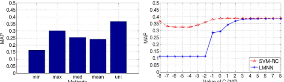
We show first in Fig. 1 left and Fig. 2 left the baseline performance. The first 4 bars in both plots show the minimum, maximum, median, and mean of the performance of the base kernels; while the last bar indicates the performance of the uniformly weighted sum of the base kernels. For the Oxford Flower17 dataset, the uniform weighting scheme outperforms the best single kernel by a large margin (0.3680 vs. 0.3022); while for the Caltech101 dataset, its advantage is only marginal (0.2303 vs. 0.2294).
In Fig. 1 right and Fig. 2 right we show the performance of the global version of the proposed MKL via SVM-RC and MKL via LMNN schemes. For the global
2
Fig. 1.Oxford Flower17. Left: baseline. Right: performance of global learning.
Fig. 2.Caltech101. Left: baseline. Right: performance of global learning.
version, triplets of relative comparison are drawn randomly from the 1020 images in the database. Note that this is not realistic since in a retrieval scenario the labels of the images in the database are not available. Nevertheless, we present the results of the global learning schemes to show the advantage of localised learning.
For both global schemes we use approximately the same number of triplets for training. For MKL via SVM-RC, we randomly draw 2×10⁴ triplets of samples such that two samples share the same label and the third one has a different label. For the MKL via LMNN scheme, we first randomly draw 100 samples as samplei. We then identify for each of them the nearest 3 samples with the same label, which form samplej. Finally, 70 samples are randomly drawn for each of the 100 “isamples” from those with different labels, and are used as samplek. This process results in 100×3×70 = 2.1×10⁴triplets. With∼2×10⁴triplets, both methods use several GB of memory, and take∼15 seconds to learn a set of kernel weights on a single core processor.
Fig. 3.Oxford Flower17. Learnt kernel weights in the global version of MKL via SVM-RC and MKL via LMNN.C= 108.
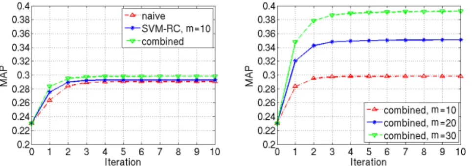
Fig. 4.Oxford Flower17. Localised learning for relevance feedback. Left: naive, learning based, and combined schemes,m= 10. Right: combined scheme,m= 10,20,30.
Fig. 5. Caltech101. Localised learning for relevance feedback. Left: naive, learning based, and combined schemes,m= 10. Right: combined scheme,m= 10,20,30.
We vary the value of the trade-off parameterCin both schemes from 10−8to 108, and show in Fig. 1 right and Fig. 2 right how the performance varies accord-ingly. Results on both datasets show that for SVM-RC, whenC is sufficiently small, the learnt kernel weights are uniform, leading to an MAP that is same as the uniform weighting scheme. For LMNN, whenC is sufficiently small, the learnt kernel weights are all zeros, which means its performance becomes that of a random distance metric. For both methods, the optimal performance is reached whenC is large enough. WhenC= 108, the MAPs of SVM-RC and LMNN for-mulations on the Oxford Flower17 dataset are 0.3892 and 0.3845 respectively, as compared to 0.3680, which is the MAP achieved by uniform weighting. The learnt kernel weights in both global schemes whenC= 108are shown in Fig. 3. On the Caltech101 dataset, similar improvements are observed (0.2553/0.2462 vs. 0.2303).
In the following experiment we turn to localised learning for relevance feed-back. We draw triplets following the scheme outlined in Section 3.2. These “local triplets” are then used for learning a distance metric for this particular query image. Since the number of images a user labels,m, is typically small, the effect of pulling all similarly labelled samples and that of pulling only the nearestgof them become similar. Therefore, we show only the results of localised MKL via
SVM-RC. Note that since we have the labels of the images in the benchmark dataset, the manual labelling process is simulated.
In addition to learning a distance metric, another way of using the labels provided by the user is simply to rank the positively labelled samples at the top of the list of retrieved images. We shall call this the naive scheme. Furthermore, this naive scheme can be combined with the learning based scheme: we learn a new distance metric using the labelled samples, retrieve again with the new metric, and then rank the positively labelled samples at the top of the new list. We shall call this the combined scheme in the following experiment.
The relevance feedback procedure can be applied iteratively. In each round, the newly labelled images are pooled with the labelled images in the previous rounds for triplet sampling, and a new distance metric is learnt, which will be used for retrieval in the next round. This allows a user to actively explore the database and improve the metric used for retrieval.
The performance of the three schemes: naive, learning based (localised MKL via SVM-RC), and combined, is plotted in Fig. 4 left and Fig. 5 left, where iteration 0 corresponds to uniform weighting of kernels. In the learning based scheme, the trade-off parameter C is set to 108, and the number of randomly sampled triplets is set to 103. It is clear from the figures that both the combined scheme and the learning based scheme outperform the naive scheme. This means that significant improvements are indeed from learning the kernel weights.
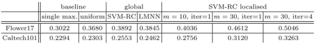
In Fig. 4 right and Fig. 5 right we show the performance of the combined scheme with various numbers of labelled images. As expected, the performance improves significantly as the number of manually labelled samples increases. La-belling even 30 images is fast as the user needs to indicate either the relevant or irrelevant images only. Finally, the MAPs of all methods under comparison on both datasets are summarised in Table 1. Note that the MAPs of localised learn-ing are achieved without combinlearn-ing with the naive scheme. We can see from the table that the localised learning scheme not only outperforms the baseline meth-ods, but also outperforms global learning. With 103triplets at each iteration, it takes on average 0.061 seconds to learn the kernel weights.
Table 1.Performance on both datasets: a summary baseline global SVM-RC localised
single max. uniform SVM-RC LMNNm= 10, iter=1m= 30, iter=1m= 30, iter=4 Flower17 0.3022 0.3680 0.3892 0.3845 0.4036 0.4612 0.5046 Caltech101 0.2294 0.2303 0.2553 0.2462 0.2756 0.3120 0.3263
5
Conclusions
In this paper we have formulated multiple kernel learning as a distance metric learning problem. We consider two objective functions that are commonly used in
distance metric learning, and optimise them under constraints based on relevance comparisons. We have proposed both global version and localised version of such a MKL via DML scheme. We argue that the localised version not only yields better performance than the global version, but also fits naturally into the framework of example based retrieval and relevance feedback. This claim is verified through experiments on two image retrieval datasets.
Acknowledgement
We would like to acknowledge support for this work from the EPSRC/UK grant EP/F069626/1 ACASVA Project.
References
1. J. Shawe-Taylor and N. Cristianini,Kernel Methods for Pattern Analysis. Cam-bridge University Press, 2004.
2. G. Lanckriet, N. Cristianini, P. Bartlett, L. E. Ghaoui, and M. Jordan, “Learning the kernel matrix with semidefinite programming,”JMLR, vol. 5, pp. 27–72, 2004. 3. F. Bach and G. Lanckriet, “Multiple kernel learning, conic duality, and the smo
algorithm,” inICML, 2004.
4. S. Sonnenburg, G. Ratsch, C. Schafer, and B. Scholkopf, “Large scale multiple kernel learning,”JMLR, vol. 7, pp. 1531–1565, 2006.
5. E. Xing, A. Ng, M. Jordan, and S. Russell, “Distance metric learning, with appli-cation to clustering with side-information,” inNIPS, 2002.
6. M. Schultz and T. Joachims, “Learning a distance metric from relative compar-isons,” inNIPS, 2004.
7. K. Weinberger and L. Saul, “Distance metric learning for large margin nearest neighbor classification,”JMLR, vol. 10, pp. 207–244, 2009.
8. M. Kloft, U. Brefeld, S. Sonnenburg, and A. Zien, “Efficient and accurate lp-norm mkl,” inNIPS, 2009.
9. J. Ye, S. Ji, and J. Chen, “Multi-class discriminant kernel learning via convex programming,”JMLR, vol. 9, pp. 719–758, 2008.
10. F. Yan, K. Mikolajczyk, M. Barnard, H. Cai, and J. Kittler, “Lp norm multiple kernel fisher discriminant analysis for object and image categorisation,” inCVPR, 2010.
11. S. Yan, D. Xu, B. Zhang, H. Zhang, Q. Yang, and S. Lin, “Graph embedding and extensions: A general framework for dimensionality reduction,”PAMI, 2007. 12. M. Nilsback and A. Zisserman, “Automated flower classification over a large
num-ber of classes,” in Indian Conference on Computer Vision, Graphics and Image Processing, 2008.
13. L. Fei-Fei, R. Fergus, and P. Perona, “One-shot learning of object categories,”
PAMI, vol. 28(4), pp. 594–611, 2006.
14. K. Sande, T. Gevers, and C. Snoek, “Evaluation of color descriptors for object and scene recognition,” inCVPR, 2008.
15. K. Grauman and T. Darrell, “The pyramid match kernel: Discriminative classifi-cation with sets of image features,” inICCV, 2005.
16. S. Lazebnik, C. Schmid, and J. Ponce, “Beyond bags of features: Spatial pyramid matching for recognizing natural scene categories,” inCVPR, 2006.