Stochastic Modeling of Future Highway Maintenance Costs for Flexible Type Highway Pavement Construction Projects

(1)

STOCHASTIC MODELING OF FUTURE HIGHWAY

MAINTENANCE COSTS FOR FLEXIBLE TYPE

HIGHWAY PAVEMENT CONSTRUCTION PROJECTS

A Thesis by

YOO HYUN KIM

Submitted to the Office of Graduate Studies of Texas A & M University

in partial fulfillment of the requirements for the degree of MASTER OF SCIENCE

May 2012

(2)

STOCHASTIC MODELING OF FUTURE HIGHWAY

MAINTENANCE COSTS FOR FLEXIBLE TYPE

HIGHWAY PAVEMENT CONSTRUCTION PROJECTS

A Thesis by

YOO HYUN KIM

Submitted to the Office of Graduate Studies of Texas A & M University

in partial fulfillment of the requirements for the degree of MASTER OF SCIENCE

Approved by:

Chair of Committee, Kunhee Choi Committee Members, .. Sarel Lavy

Sarah Deyong Head of Department, Joe Horlen

May 2012

(3)

iii

ABSTRACT

Stochastic Modeling of Future Highway Maintenance Costs for Flexible Type Highway Pavement Construction Projects.

(May 2012)

Yoo Hyun Kim, B.A., Hongik University Chair of Advisory Committee: Dr. Kunhee Choi

The transportation infrastructure systems in the United States were built between the 50's and 80's, with 20 years design life. As most of them already exceeded their original life expectancy, state transportation agencies (STAs) are now under increased needs to rebuild deteriorated transportation networks. For major highway maintenance projects, a federal rule enforces to perform a life-cycle cost analysis (LCCA).

The lack of analytical methods for LCCA creates many challenges of STAs to comply with the rule. To address these critical issues, this study aims at developing a new methodology for quantifying the future maintenance cost to assist STAs in performing a LCCA. The major objectives of this research are twofold: 1) identify the critical factors that affect pavement performances; 2) develop a stochastic model that predicts future maintenance costs of flexible-type pavement in Texas.

(4)

iv The study data were gathered through the Pavement Management Information

System (PMIS) containing more than 190,000 highway sections in Texas. These data were then grouped by critical performance-driven factor which was identified by K-means cluster analysis. Many factors were evaluated to identify the most critical factors that affect pavement maintenance need. With these data, a series of regression analyses were carried out to develop predictive models. Lastly, a validation study with PRESS statistics was conducted to evaluate reliability of the model. The research results reveal that three factors, annual average temperature, annual precipitation, and pavement age, were the most critical factors under very low traffic volume conditions.

This research effort was the first of its kind undertaken in this subject. The maintenance cost lookup tables and stochastic model will assist STAs in carrying out a LCCA, with the reliable estimation of maintenance costs. This research also provides the research community with the first view and systematic estimation method that STAs can use to determine long-term maintenance costs in estimating life-cycle costs. It will reduce the agency’s expenses in the time and effort required for conducting a LCCA. Estimating long-term maintenance cost is a core component of the LCCA. Therefore, methods developed from this project have the great potential to improve the accuracy of LCCA.

(5)

v

DEDICATION

Send my unlimited affection to my family

Kwangwon Kim Haesook Park

Kahye Oh Jungyoon Kim

(6)

vi

ACKNOWLEDGEMENTS

I would like to express my gratitude to my committee chair, Dr. Kunhee Choi, for his encouragement, insightful directions and guidance over the course of this research study. I would also like to extend my sincere thanks to my committee members, Dr. Sarel Lavy and Dr. Sarah Deyong, for their invaluable advice and comments. I strongly believe that I was able to improve analyses and my knowledge further due to their insightful comments.

Especially, I would like to send my sincere thanks to Jeongho Oh, a researcher, Texas Transportation Institute (TTI), for his valuable material and advice. In addition, I would like to sincerely thank my colleagues, Ji-myong Kim, Kyeongbong Han and Sangguk Yum, who helped me complete the thesis in a timely manner. Also, I would like to send my special thanks to Mrs. Carleen Cook who has served as my counselor and tutor, especially on helping to improve my technical writing skills. Finally, I am grateful to my parents for their tireless support and wish them the best for their good health and spirits.

(7)

vi

i

NOMENCLATURE

AADT Annual Average Daily Traffic

AASHTO American Association of State Highway and

ACP Asphalt Concrete Pavement

ADT Average Daily Traffic

ANOVA Analysis of Variance

ARRA Act American Recovery and Reinvestment Act Caltrans California Department of Transportation

CRCP Continuous Reinforced Concrete Pavement

JCP Jointed Concrete Pavement

FHWA Federal Highway Administration

HMA Hot Mixed Asphalt

IH Interstate Highway

IRI International Roughness Index

LCCA Life Cycle Cost Analysis

NHS National Highway System

PCI Pavement Condition Index

PSI Pavement Serviceability Index

RSL Remaining Service Life

SH State Highway (or SR: State Route)

(8)

vi

ii

(9)

ix

DEFINITION OF TERMS

Lane-mile The total length of all lanes calculated as centerline mile multiplied by the number of lanes

Routine Maintenance Defined in “Maintenance Management Manual” issued by TxDOT in 2008. Include pavement repair, crack seal, seal coat, level-ups, light overlay less than 2 inches and additional base. Normally, contract amount should not exceed $300,000 per project. (Table 3)

Preventive Maintenance Defined in PMIS. Include crack seal and surface seal. In case of thin asphalt, cost is less than $8,000 per lane-mile and in case of med or thick asphalt, cost is less than $10,000 per lane-mile (Table 4).

(10)

x

LIST OF FIGURES

Page

Figure 1. Highway maintenance work-frame ... 11

Figure 2. Example of typical pavement M&R schedule in Caltrans (Caltrans 2007) ... 20

Figure 3. Flexible pavement structure (Rogers 2003) ... 25

Figure 4. Survival time versus Overlay thickness (Yu et al. 2008) ... 28

Figure 5. Survival time versus Log-ADT (Yu et al. 2008) ... 31

Figure 6. PMIS data exported to Microsoft Access ... 35

Figure 7. Data stratification procedure ... 40

Figure 8. Scatter plot of maintenance cost versus annual average temperature ... 44

Figure 9. Scatter plot between maintenance cost versus annual average precipitation ... 45

Figure 10. Scatter plot between maintenance cost versus pavement thickness ... 46

Figure 11. Scatter plot between cost versus traffic volume ... 47

Figure 12. Scatter plot between maintenance cost versus pavement age ... 48

Figure 13. Residual plot for outlier detection ... 50

Figure 14. Residual plot of initial regression analysis ... 51

Figure 15. Transformed results analyzed from Box-Cox ... 52

Figure 16. Transformed regression residual plot ... 53

Figure 17. Transformed results analyzed by Box-Cox ... 57

Figure 18. Residual plot of cluster 1 ... 58

(14)

xi

v

LIST OF TABLES

Page

Table 1. Categorized climate region used in California (Caltrans 2007) ... 6

Table 2. Total lane-mile of Texas highways in 2005 (Mikhail et al. 2006) ... 15

Table 3. Maintenance categories defined in Maintenance Management Manual (TxDOT 2008) ... 23

Table 4. PMIS maintenance types and costs defined in PMIS (Stampley et al. 1993) ... 24

Table 5. Data sorted from PMIS (DYE Management Group 2006) ... 37

Table 6. Pavement thickness converting criteria ... 39

Table 7. Data range after phase 2 classification ... 41

Table 8. Descriptive Statistics ... 43

Table 9. Correlation analysis ... 49

Table 10. Regression Model Summary ... 50

Table 11. Transformed regression summary ... 52

Table 12. K-means clustered results ... 55

Table 13. Correlation analysis results for cluster 1 ... 56

Table 14. Outlier detection process through Casewise Diagnostics ... 59

Table 15. ANOVA Table of regression model for cluster 1 ... 59

Table 16. Coefficients of transformed model for cluster 1 ... 60

Table 17. Correlation analysis results for cluster 2 ... 63

Table 18. Outlier detection process through Casewise Diagnostics ... 65

(15)

xv Page

Table 20. Coefficient of Transformed model for cluster 2 ... 66 Table 21. The PRESS statistic versus the SSE of the cluster 1 model ... 72 Table 22. Maintenance cost trend in the first year for cluster 1 ... 77

(16)

1

1 INTRODUCTION

1.1 Needs for Highway Infrastructure Recovery

During the construction boom between the 1950’s and 1980’s, most transportation infrastructure systems were established with a 20-year life expectancy (FHWA 2002; Lee and Ibbs 2005). After the 2000’s, these highways have created severe public concerns with regard to safety and regional economic problems. Since most highways in the US have already exceeded their design life expectancy, a huge amount of money is necessary to restore the nationwide highway infrastructure. However, the recent economic recession has created a poor financial status in many state governments which has made it impossible to increase governmental expenditures for infrastructure recovery projects. Under this situation, the American Recovery and Reinvestment Act (ARRA Act) was enacted in February 2009 by the Obama Administration and the US Congress which has included many projects to improve poor systems and plan for large scale investments. The major points for improving highway infrastructure can be summarized as investment of a huge amount of federal money into the infrastructures, up to $80 billion, to promote the recovery of highways from their present status and stimulate the regional and national economies through federal investment.

This thesis follows the style of the Journal of Construction Engineering and Management.

(17)

2

1.2 Needs of LCCA for Transportation Projects

The Federal Highway Administration (FHWA) strongly recommends using Life-Cycle Cost Analysis (LCCA) for most highway projects for new projects and 4R projects: restoration, resurfacing, rehabilitation and reconstruction (FHWA 2002). LCCA methodologies are a comprehensive tool for decision making by comparing cost efficiency between design alternatives (FHWA 2002). To analyze life-time cost for infrastructure, maintenance cost data is the most essential of many cost factors since one-time cost is only a small part of the total cost for a life time. Generally, factors such as initial cost, operating cost, maintenance and replacement cost and salvage value are included in LCCA. Especially, maintenance and rehabilitation projects (M&R) comprise a large proportion in early step of projects (FHWA 2002). Therefore, exact data for M&R costs are essential to produce more exact LCCA for many design alternatives and to make an efficient decision.

(18)

3

2 RESEARCH SCOPE AND SIGNIFICANCE

2.1 Gaps in Existing Knowledge

2.1.1 Introduction of RealCost

RealCost is a computer software which analyzes the life-cycle cost of highway projects. If various factors are entered into the software, LCCA is computed automatically and the software shows comparisons in regard to all alternatives of a project. This software has been designated as one analysis tool in FHWA for two major purposes: to provide an instructional and educational tool for decision makers in pavement design and to provide a practical tool for pavement designers who can use the results when developing pavement plans (FHWA 2004). The software compute life-cycle values for both agency and user costs at the same time with regard to rehabilitation projects as well as new construction. Also, it provides deterministic and probabilistic modeling of LCCA. One important function of the RealCost compares results of alternatives to analyze the advantages and disadvantages of many alternatives. However, even though this software provides analyzed cost data from various angles, the output from the RealCost isn’t the only crucial factor for decision making since there are many other factors to consider such as risks, available budget, political situations and environmental issues. Therefore, even though RealCost provides critical information for the overall decision making process, as an economic analysis tool, the optimized output from RealCost is just one solution of many alternatives (FHWA 2004).

(19)

4 The California Department of Transportation (Caltrans) is one of the leading State

Agencies (STAs) using and developing LCCA. RealCost manual issued by Caltrans provides background data which includes maintenance and rehabilitation cost during the pavement’s life cycle by considering various regional, climatic and physical aspects of highways which are critical factors for computing life-time costs. In other words, the level of accuracy and classification of the background data determines the quality of LCCA.

2.1.2 Problems in Present Life-Cycle Cost Analysis

Poorly managed highway infrastructure is one of the public issues in the US even though highway infrastructure influences the national economy in many ways (Choi and Kwak 2011; Shatz et al. 2011) As one way to escape from the present recession, the Obama administration has decided to invest a huge amount of money to reform highway infrastructure and STAs are needed to increase efficiency in these budget allocation and management. As a decision support tool, LCCA has been used for comparing alternatives, decision making and budget allocation in many STAs (Salem et al. 2003). In addition, much research has been conducted to develop LCCA methodologies. However, STAs depend on background data for LCCA from their individual empirical data. There are no established criteria at the nationwide level, even though critical cost elements determining life cycle costs including routine maintenance costs are essential to provide more exact life time costs. Especially, routine maintenance costs have wide variability influenced by environmental,

(20)

5 regional and physical conditions of pavement in a number of ways. Thus, routine

maintenance cost prediction methodologies should be developed based on various factors and should be studied to provide more exact prediction of life time cost for highway recovery projects.

2.1.3 Limitation of LCCA Tools

There have been many trials to establish systems to support decision making for new construction or rehabilitation highway projects such as LCCA tools, planning tools and design tools. Specifically, LCCA tools like RealCost provide useful economic information to decide highway design and choose among many alternatives. However, one problem is whether or not these LCCA tools have sufficient background data to support reliable results. The California Department of Transportation (Caltrans), leading LCCA development and usage, has developed M&R cost schedules but categories representing climate regions are divided into five sectors for maintenance and rehabilitation (M&R) schedule as shown in Table 1. Moreover, the planned maintenance costs are same year by year in the table of pavement M&R Schedules which is a major database for RealCost. As a result, these limitations make it difficult to plan annual budget allocations. Since LCCA is not only for decision making for initial projects, but for whole life cycle costs and cash flow analysis, this limitation has clearly become an obstacle for developing detailed and exact analyses for life cycle costs of a project.

(21)

6 Table 1. Categorized climate region used in California (Caltrans 2007)

California Climate Regions Categorized by Caltrans

Climate Regions for Pavement M&R Schedule

Used in Caltrans North Coast

All Coastal Central Coast

South Coast

Inland Valley Inland Valley High Mountain

High Mountain & High Dessert High Dessert

Desert Desert

Low Mountain

Low Mountain & South Mountain South Mountain

2.2 Research Objectives

Objective 1: Collect reliable highway maintenance data for Texas Objective 2: Identify critical factors influencing pavement conditions

Objective 3: Identify relationships between routine pavement maintenance costs and identify factors impacting pavement condition

Objective 4: Provide lookup tables for the routine pavement maintenance costs categorized based on identified factors.

(22)

7

2.3 Research Methodologies and Hypothesis

2.3.1 Tasks to Achieve Research Objectives

Task 1: Identify physical and environmental factors impacting pavement condition. Task 2: Collect reliable data for identified factors and maintenance cost

Task 3: Test the relationships between identified factors and maintenance cost Task 4: Create a maintenance cost prediction model using statistical method Task 5: Test validity of the model through comparison with other highway data Task 6: Provide lookup tables based on each categorized factor.

2.3.2 Stochastic Analysis

To provide a reliable pavement maintenance prediction model, the statistical analysis method was applied in this research step by step. The data used in this study was from the Pavement Management Information System (PMIS) which has been widely used in TxDOT and its district agencies. The following statistical procedures were implemented with PMIS data.

1. Data classification based on the research standard

According to the research scope, data should be classified and manipulated. If many independent factors are identified and it’s difficult to analyze the data trend under normal statistical methods, the data should be classified once more through clustering analysis: statistical classification methods.

(23)

8 Descriptive analysis provides basic data features for extracted samples such as

standard deviation, mean and variance. Also, scatter plots provide insight into the basic tendency of sample data.

3. Pearson and Spearman correlation test

This statistical test is to test the fundamental relationships between identified variables and the dependent variable.

4. Box-Cox analysis

If the relationship has high significance in the Spearman test, the sample data need transformation. Box-Cox analysis provides the best fit in the sample data transformation.

5. Casewise diagnostics and residual scatter plot

To increase the model’s reliability, the outliers are eliminated through checking residual scatter plots and Casewise diagnostics. Also, equal variance for the sample data can be checked through standardized residual scatter plots.

6. ANOVA test

Once regression analysis is performed and produces prediction models, this test identifies the model’s significant differences among means of variables.

7. Individual coefficient test and co-linearity analysis

The Coefficient test provides a method to check whether or not the individual dependent variable has significance with the suggested prediction model. Also, co-linearity analysis provides test methods if there are correlations between dependent variables.

(24)

9

2.3.3 Hypothesis

The specific purpose of this study was to identify:

1. If there is any relationship between identified physical and environmental factors and maintenance cost and

2. If it’s possible to predict the maintenance cost or obtain statistical tendency between the identified factors and maintenance cost

Following model was used to test this hypothesis:

Model: Mc = 𝛽0+ 𝛽1∗ 𝐴𝑡 + 𝛽2∗ 𝐴𝑝 + 𝛽3∗ 𝑃𝑡 + 𝛽4 ∗ 𝑇𝑣 + 𝛽5∗ 𝑃𝑎

At = Annual Average Temperature (°F) Ap = Annual Average Precipitation (inch)

Pt = Pavement thickness (Surfacing Thickness) (ordinal value) Tv = Traffic Volume based on Annual Average Daily Traffic (count) Pa = Pavement Age from the last surface overlay date (years) Mc = Annual Maintenance Cost per lane mile ($/lane-mile)

The suggested variables tested those influences on pavement through the literature review and could be changed based on the process of statistical analysis. This model confirms relationship between annual pavement maintenance cost and critical factors which were identified in the literature review. Annual pavement maintenance cost would be predicted based on this equation after being developed and validated.

(25)

10

2.4 Research Assumptions

 Under $10,000 of annual maintenance costs per lane mile in pavement thickness over 2.5 inches and under $8,000 annual maintenance cost per lane mile in pavement thickness under 2.5 inches are regarded as routine maintenance costs without any overlay activities (Scullion et al. 1997).

 Regional climate factors such as precipitation and temperature are the same in one county (Scullion et al. 1997).

 Typical life expectancy of ACP is 10 years and within this life expectancy, material characteristics of ACP follow expected physical characteristics.

 The sample data is normally distributed according to the Central Limit Theorem. The population of data was from PMIS having over 190,000 section data and the sample data about 1,000 section data was extracted from PMIS.

(26)

11

2.5 Limitation

 The research is limited to State Highway (SH) sections in Texas

 The research is limited to only Asphalt Concrete Pavement (ACP)

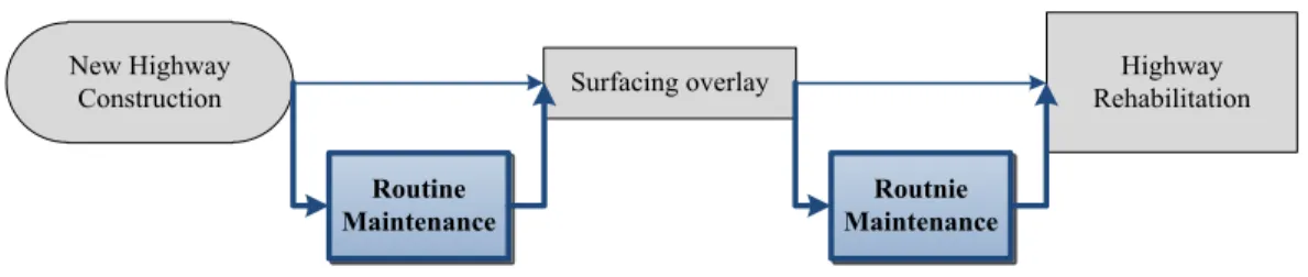
 The research is limited to only routine maintenance costs, not including surfacing overlay or rehabilitation costs. For long pavement life, there are several recovery strategies which are classified differently by system, STAs and definitions. In this research, the routine maintenance concept was shown in Figure 1.

Figure 1. Highway maintenance work-frame

 The original source of data for this research is from TxDOT’s Pavement Management Information System (PMIS) which is under development. Thus, imperfections in PMIS such as omissions in data have influenced the result of this study.

Surfacing overlay _{Rehabilitation}Highway New Highway

Construction

Routine

(27)

12

2.6 Significance of the Research

This research will be of significance to the highway agencies located in Texas since the objective is to provide detailed maintenance cost data based on identified factors which can be utilized in LCCA for their decision making and annual budget allocations. The research unveils whether or not raw factors such as environmental conditions and physical features of pavement affect maintenance costs representing pavement management practices. Moreover, the pavement maintenance cost prediction model is suggested by using statistical methodology which connects identified environmental factors and maintenance costs. That is, this study is one trial to make a connection between two fields of studies: engineering studies and management practices.

(28)

13

3 LITERATURE REVIEW

The purpose of the literature review was to understand related studies including engineering and maintenance practices for life-cycle-cost analysis of highway projects. Specifically, the literature review was conducted to identify critical factors impacting routine highway maintenance costs in Texas and to investigate current LCCA practices used for comparison and decision making between highway project alternatives.

3.1 Highway Facts

There are several types of roadway systems in the United States classified as functional system, ownership, location and federal-aid or no federal-aid roadways (FHWA 2008). Fundamental Highway classification is a functional classification system established in 1989 by the Federal Highway Administration (FHWA). This system comprises three blocks such as local roads, collectors and arterials. Sometimes, Freeway/Expressway is included in this categorization to separate heavy traffic highways from arterial roads. Local roads are for homes, businesses, farms and small communities and provide channels to collector roadways. The major function of collectors is to provide access from local roads to arterials and arterial roads connecting between towns and cities (FHWA 2011).

Among these highway systems, the FHWA has classified National Highway system (NHS) according to the importance of the national economy, defense and mobility.

(29)

14 All interstate highways (IH), the Strategic Highway Network, intermodal connectors

and other principal arterials belong to NHS whose total length is about 166,000 miles but occupies only 4% of the US roadway systems and carries more than 40% of all highway traffic, 75% of heavy truck traffic and 90% of tourist traffic (Slater 1996).

Several government organizations have ownership of roadways: the Federal Agency, State Highway Agency (STA), County, Town or other jurisdictions. These institutions generally have rights and responsibilities of their owned roadways (FHWA 2008)

Roadway location is one of the standards to classify roadways into “Urban” area roadways and “Rural” area roadways. Since the increase and spread of population, there is a general trend to decrease rural area roadways (FHWA 2008).

Another way to categorize roadway is whether or not there is federal government support. Federal aid roadways include the National highway system; if the roadways don’t have any federal supports, they are classified as non-federal-aid roadways. These classifications are combined to analyze many aspects and to make up annual statistical data for roadways in the United States.

In Texas, there are four major highway types such as Interstate Highway (IH), US route (US), State Highway/Route (SH or SR) and Farm to Market Road (FM).

(30)

15 Generally, IH and US are classified as National Highway System (NHS). SH and FM

are classified as highways under local government agencies. Most highways including IH and US are owned by state governments (FHWA 2008), but management and design criteria for these highways is still under FHWA control. In case of SH and farm to market roads, various standards are under local government rules such as state, municipal and county governments. Particularly, these criteria for SH follow rules of the Texas state government and state highway agency.

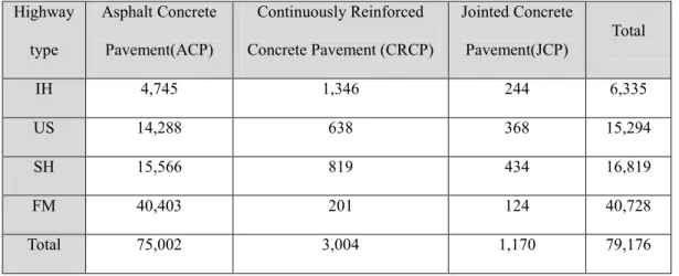
Texas is one of the largest states in the United States. Accordingly, Texas has a huge highway system to manage which is total 79,000 lane mile. Paved lane-miles of major highways in Texas are as shown in Table 2.

Table 2. Total lane-mile of Texas highways in 2005 (Mikhail et al. 2006)

Highway type Asphalt Concrete Pavement(ACP) Continuously Reinforced Concrete Pavement (CRCP) Jointed Concrete Pavement(JCP) Total IH 4,745 1,346 244 6,335 US 14,288 638 368 15,294 SH 15,566 819 434 16,819 FM 40,403 201 124 40,728 Total 75,002 3,004 1,170 79,176

(31)

16

3.2 Highway Management Studies

Many highways which have exceeded in their 20 years design life expectancy have created critical challenges for State Transportation Agencies. Even though most highways were constructed from 1960s to 1980s during a construction boom, much of the overage pavement in these highways is still in use (Lee and Ibbs 2005). In consequence, the improvement of transportation infrastructure became one of the fourteen grand challenges for engineering in the 21st century by the National Academy of Engineering under the Obama administration which passed the

American Recovery and Reinvestment Act of 2009 (ARRA act). The purpose of the ARRA act and selection of the 14 engineering challenges was to provide investment in infrastructure, education, health and green energy.

Out of these plans, the amount of federal investment in highway recovery projects is about $80 billion but there are many serious problems related to the economy of new construction and traffic disruptions. So, with FHWA and State Highway agencies, the paradigm for highway construction has turned from new construction to maintenance and renewal of existing facilities represented as 4R: restoration, resurfacing, rehabilitation and reconstruction (Choi and Kwak 2011; Lee and Ibbs 2005).

In 2008, national total disbursements for physical maintenance of state administered highways were $12,499,324,000. Out of this expenditure, Texas spent $1,300,886,000 for roadway physical maintenance during one year (FHWA 2008). In

(32)

17 general, one district in Texas spends an average of $52,000,000 per year which is the

sum of combined contracted and non-contracted maintenance expenditures (TxDOT 2011). Clearly, each district invests huge amount of money annually to maintain highway system which is major transportation infrastructure.

Pavement maintenance is highly related to safety, serviceability and efficiency of highways. Pavement damage caused by traffic loads and environmental influences worsen the performance of highways. So, pavement maintenance on a regular basis is critical to maintain and improve pavement performance and quality (Embacher and Snyder 2001; Labi and Sinha 2005). Inadequate budget allocations for pavement maintenance regardless of heavy use and environmental conditions is often ineffective and cause wasted resources in spite of STAs’ limited financial situation of agencies (Labi and Sinha 2005). Moreover, not only maintenance costs but rehabilitation costs increase due to failure of efficient decision making. Therefore, it’s essential to maintain pavement in a timely and effective way (Chou and Le 2011).

Life Cycle Cost Analysis (LCCA) is one way to improve efficiency in highway construction activities including new construction as well as 4R projects (Labi and Sinha 2005). As an engineering economic analysis tool and a decision-support tool, LCCA is useful to compare project alternatives. From the Intermodal Surface Transportation Equity Act of 1991, implementing LCCA in highway investment decisions has been one of the main policies that FHWA encourages (FHWA 2002).

(33)

18 It’s highly recommended that LCCA be completed as early as possible. Especially, in

all California highway projects supervised by Caltrans, LCCA must be performed based on established procedures and data in the LCCA procedure manual issued by Caltrans. Fundamental steps for LCCA are as follows: 1. Establish Design Alternatives 2. Determine Activity timing 3. Estimate Costs including agency and user costs 4. Compute life-cycle costs 5. Analyze the results (FHWA 2004).

There are two different computational approaches in LCCA: Deterministic and Probabilistic. First, the deterministic approach is the recommended and traditional way for project decision-support (Caltrans 2007). In this approach, each input variables for LCCA should be fixed and separated. These variables can generally be determined based on historical evidence or professional judgment (Caltrans 2007). On the contrary, a probabilistic approach is a relatively new methodology based on uncertainty and variation with regard to input variables (FHWA 2002) . Compared with an individual computation of the deterministic approach, the probabilistic approach has advantages because different assumptions for uncertain variables based on probability distribution can be included in the computation at the same time. However, the probabilistic methodology has been under-developed until now and many STAs and FHWA don’t recommend this method as yet (Caltrans 2007; FHWA 2002). So, Agencies allow only the deterministic approach for LCCA in highway projects at this time (Caltrans 2007).

(34)

19 To perform a LCCA in a certain project, necessary factors are as follows:

1. Design alternatives 2. Analysis period 3. Discount rate

4. Maintenance and rehabilitation sequences 5. Costs

6. RealCost software

Among these factors, costs include initial costs (construction costs and project support costs), maintenance costs, rehabilitation costs and user costs (Caltrans 2007). Also, maintenance costs are comprised of costs for routine, preventive and corrective maintenance such as sealing, void under sealing, chip sealing, patching, spall repair, individual slab replacement, thin hot mix asphalt overlay, etc (Stampley et al. 1993; TxDOT 2008). In case of Caltrans, annualized maintenance costs are used and this historical cost data is collected by the Division of Maintenance. Following Figure 2 is an example of maintenance costs used by Caltrans.

(35)

20

(36)

21 The federal highway agency strongly recommends the use of LCCA in the early

stage of highway construction projects and in some states LCCA is a mandatory process in the pre-construction stage of highway projects (FHWA 2002). Obviously, LCCA methodology provides a clear insight into life time cost allocations for highway agents who try to predict budget expenses and their allocation.

However, even the most advanced users of LCCA methodology have used a relatively undetailed maintenance costs index based on a few categorized climate regions (Table 1). Moreover, annual maintenance costs are the same all the time until and even after roadway rehabilitation. This means that these data ignore many factors such as traffic volume, pavement age and annual interest rate. With this data, it’s incorrect to predict and allocate annual maintenance costs of each highway. Due to at least 20 years pavement life expectancy, annual maintenance cost is the main factor used to analyze more exact life time costs and annual budget allocations with both deterministic and probabilistic life-cycle cost analysis. Especially, to improve reliability for the probabilistic approach in highway LCCA, more detailed and categorized maintenance costs are necessary.

(37)

22

3.3 Maintenance Practice and Criteria

Texas Department of Transportation (TxDOT) has established several standards for pavement maintenance based on procedure, range, type and budget amount. These standards should be referred to whenever highway agencies make plans or decisions for highway maintenance. First of all, pavement maintenance should be implemented based on the following six phases: planning, budgeting, scheduling, performing, reporting and evaluating (DYE Management Group 2006). All maintenance processes should be carried out according to highway maintenance plans established and revised on an annual basis to obtain more realistic plans.

Fundamentally, there are three kinds of plans categorized by length of term: annual plans, four year plans and long-range transportation plans. Annual plans primarily focus on actual pavement management. In contrast to the annual plan, the four year plan and the Texas long-range transportation plan are conceptual and directional plans for improving all transportation systems over designated periods (Gao et al. 2011; Scullion et al. 1997; TxDOT 2009; TxDOT 2010).

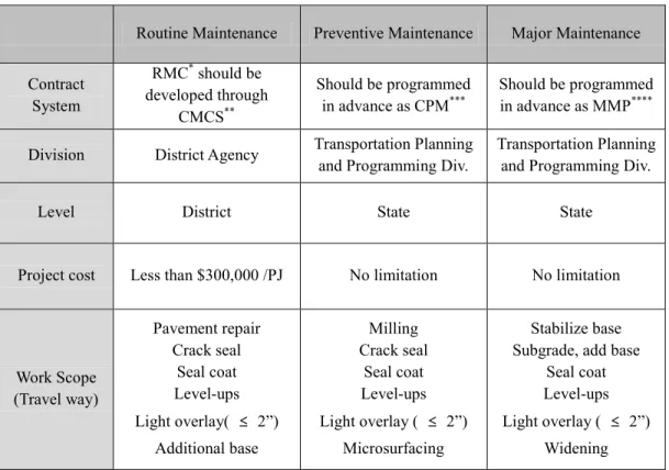
TxDOT categorizes maintenance work into three areas: routine maintenance, preventive maintenance and major maintenance. Most preventive and major maintenance work should be contracted but routine maintenance works can be performed by either the agency’s force or contract (Embacher and Snyder 2001; TxDOT 2008). In addition to this, each maintenance scope is managed by a different

(38)

23 division or program with a different budget range and different work scope as shown

on the following table.

Table 3. Maintenance categories defined in Maintenance Management Manual (TxDOT 2008)

Routine Maintenance Preventive Maintenance Major Maintenance Contract System RMC*_{should be} developed through CMCS** Should be programmed in advance as CPM*** Should be programmed in advance as MMP**** Division District Agency Transportation Planning

and Programming Div.

Transportation Planning and Programming Div.

Level District State State

Project cost Less than $300,000 /PJ No limitation No limitation

Work Scope (Travel way) Pavement repair Crack seal Seal coat Level-ups Light overlay( ≤ 2”) Additional base Milling Crack seal Seal coat Level-ups Light overlay ( ≤ 2”) Microsurfacing Stabilize base Subgrade, add base

Seal coat Level-ups Light overlay ( ≤ 2”)

Widening RMC*: Routine Maintenance Contract

CMCS**: Construction/Maintenance Contract System CPM***: Contract Preventive Maintenance

MMP****: Major Maintenance Program

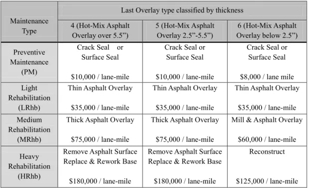
Within PMIS, four maintenance categories are defined: preventive maintenance, light rehabilitation, medium rehabilitation and heavy rehabilitation or reconstruction (Stampley et al. 1993). This category is different from the three categorized maintenance work scopes defined in the Maintenance Management Manual issued

(39)

24 by TxDOT in 2008. In addition, the work scope and cost of each maintenance

category follow the rules of PMIS itself.

Table 4. PMIS maintenance types and costs defined in PMIS (Stampley et al. 1993)

Maintenance Type

Last Overlay type classified by thickness 4 (Hot-Mix Asphalt Overlay over 5.5”) 5 (Hot-Mix Asphalt Overlay 2.5”-5.5”) 6 (Hot-Mix Asphalt Overlay below 2.5”) Preventive Maintenance (PM) Crack Seal or Surface Seal $10,000 / lane-mile Crack Seal or Surface Seal $10,000 / lane-mile Crack Seal or Surface Seal $8,000 / lane mile Light Rehabilitation (LRhb)

Thin Asphalt Overlay $35,000 / lane-mile

Thin Asphalt Overlay $35,000 / lane-mile Medium

Rehabilitation (MRhb)

Thick Asphalt Overlay $75,000 / lane-mile

Mill & Asphalt Overlay $60,000 / lane-mile Heavy

Rehabilitation (HRhb)

Remove Asphalt Surface Replace & Rework Base $180,000 / lane-mile

Reconstruct

$125,000 / lane-mile

Like the above mentioned systems, maintenance scope and range differ according to the purpose of the maintenance systems. Particularly, the concept and work scope of preventive maintenance defined in PMIS are similar to the routine maintenance work scope in the Maintenance Management Manual except for light overlay, level-ups and additional base work. These different scopes and standards can possibly cause inefficiency and confusion in an agency’s work processes. Inversely, the large number of systems established to develop efficiency in managing highways creates many possibilities for inefficiency, inversely. Thus, clear and united standards seem

(40)

25 to be necessary to increase system unity and decrease the complexity inherent in

connecting between huge numbers of systems.

Since the data source for this research came from PMIS and the objectives of this research -routine maintenance cost prediction except overlay- were closer to the concept of PMIS, the data scope for their research analysis has followed the PMIS standard.

3.4 Highway Engineering Studies

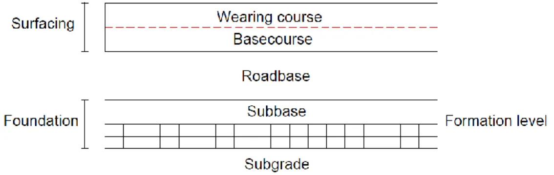
As described in Figure 3, fundamentally, there are three basic components in the pavement structure: foundation, road-base and surfacing. In a flexible-type pavement, the surfacing includes wearing course and base course and the foundation includes sub-base and subgrade (Rogers 2003).

(41)

26 Of these layers, there are two types of surfacing: flexible type and rigid type.

Normally, flexible type means asphalt based pavement (ACP) and rigid type means concrete based pavement (CRCP). However, in PMIS, pavement type was classified in three ways: ACP, CRCP and Jointed Concrete Pavement (JCP). Basically, CRCP and JCP were included in continuous reinforced concrete pavement (CRCP) (TxDOT 2011)

Since these pavement structures are constantly exposed to daily traffic and outside environment, when agents design a highway project they must consider various factors as follows: pavement performances, traffic, roadbed soil, materials, environments, drainage, reliability, life-cycle costs and shoulder design (AASHTO 1993; Birgisson et al. 2000). Much research has been conducted to investigate the relationship between these factors and pavement conditions.

To display roadway conditions in a quantitative way, there is a representative pavement condition index, Pavement Condition Index or Rate called PCI or PCR which is often used in pavement management to measure pavement distresses (Yu et al. 2008). Aside from PCI, there are many methods and indices for measuring according to the purpose of measurement. For example, the Pavement Serviceability Index (PSI) is one way to show pavement serviceability including distress and roughness (AASHTO 1993) and the International Roughness Index (IRI) determines ride quality parameters by measuring pavement smoothness (TxDOT 2011). In

(42)

27 addition, there are different kinds of indices such as Remaining Service Life (RSL)

which predicts the expected life of the pavement until its condition doesn’t provide normal highway functions any more (Yu et al. 2008). Many agents, institution and researchers choose the indices suitable for their purpose and have been recording the result of evaluations based on the indices in their system to obtain and manage information of each roadway condition. Also, considerable engineering research related to pavement has been used these indices.

Based on PCI and RSL in asphalt concrete pavement (ACP), four parameters have significant relationships with pavement performances (Jeong 2008) and survival time of pavement: temperature, precipitation, overlay thickness, traffic loading (Yu et al. 2008). The following shows the research results of the four parameters vs. pavement survival life. This study assumes that PCI 70 is the end of the serviceability of the pavement.

(43)

28 0 2 4 6 8 10 12 14 0 1 2 3 4 5 6 7 8 9 10 M ed ian S u rvival T im e (ye ar ) Overlay Thickness (Cm)

3.4.1 Survival Life Versus Overlay Hot Mixed Asphalt (HMA) Thickness

The increase of overlay HMA in every 1 inch (2.5 Cm) results in about a half year extension of pavement service life. Moreover, for thicker HMA overlays (more than 2 inches), the increase of pavement thickness extends service life. This means that thicker pavement surfacing can be a favorable choice if the financial situation is favorable (Yu et al. 2008).

As described in Figure 4, asphalt thickness is significantly related to pavement temperature which is one of the most important factors in pavement damage. Normally, thick pavement records slightly lower temperatures than thin pavement, resulting in strong resistance to climatic factors (Wahhab and Balghunaim 1994).

(44)

29

3.4.2 Pavement Performances Versus Temperature

In design ACP, pavement temperature is a mandatory input variable to predict pavement performance which was developed by the Strategic Highway Research Program (SHRP). Pavement temperature is primarily influenced by air temperature (Solaimanian et al. 1993).

In many cases, an increase in pavement temperature causes pavement performance deterioration through loss of strength in ACP. In some cases, climatic loading becomes a far more influenetial factor than physical loading such as traffic loading (Salter and Al-Shakarchi 1989; Solaimanian et al. 1993; Wahhab and Balghunaim 1994)

However, in low temperature, ranges from 47 °F to 55 °F, a 1°C rise (1.8°F) in annual average temperature causes a one year pavement service life extension. However, these data from Ohio, whose annual average termperature is from 47 °F to 55 °F, might not be suitable for areas having temperature ranges over 60 °F (Yu et al. 2008).

Although there are many research has been based on different temperature ranges and, accordingly, provided different research results, it’s clear that temperature is a critical influence on pavement service life (Solaimanian et al. 1993; Yu et al. 2008).

(45)

30

3.4.3 Pavement Performances Versus Precipitation

Another climate factor, precipitation, also plays an important role in pavement performance (Saraf et al. 1987) and survival time. A four inches (10 Cm) increase in precipitation means a decrease as much as one year in service life. So, it can be said that an increase in annual rainfall worsen pavement conditions. Since these two climatic factors, precipitation and temperature, are the characteristics of a region which agents should consider, highway agents can apply these factors for budget allocations for highways (Rogers 2003; Yu et al. 2008).

Particularly, two climatic factors, temperature and precipitation, impact pavement performance in various ways. The pavement deterioration procedure is as follows (Kapiri et al. 2000):

1. Temperature gradients result in significant physical stress in the slabs 2. Temperature differences in pavement create cracks or joint openings

3. Moisture variation in pavement causes differential shrink from top to bottom That is, inherent pavement temperature, which is closely affected by air temperature, increases pavement cracks and moisture originated from regional rainfall or humidity catalyzes this deterioration process (Kapiri et al. 2000). Climatic factors have the most influence on pavement condition compared to physical load (Kapiri et al. 2000).

(46)

31 0 2 4 6 8 10 12 1 2 3 4 5 6 7 8 9 10 Me di an Su vi val ti m e (y ear) Log AADT

3.4.4 Survival life Versus Traffic loading

In the pavement design guide in FHWA, AASHTO and STAs, traffic loading has been the major factor to be considered in new highway construction. Relationship of these two factors is displayed in Figure 5. Actually, a ten-times increase in average daily traffic leads to a half year decrease in pavement service life. That is, degeneration in pavement conditions from heavy traffic may be canceled to some degree by increased pavement thickness (Yu et al. 2008).

Figure 5. Survival time versus Log-ADT (Yu et al. 2008)

The PMIS manual issued by TxDOT designated several factors to identify to determine if pavement maintenance is nessesary: 1. Pavement type. 2. Distress ratings. 3. Ride Score. 4. Average daily traffic per lane (ADT). 5. Roadway

(47)

32 functional class. 6. Average county rainfall (in inches per year). 7. Time since last

surface (in years) (Stampley et al. 1993). These factors were defined as critical factors in PMIS which must be included when pavement treatment is considered.

These research results show that environmental and physical factors have critical impacts on pavement condition. Of course, these studies obviously have limitations to generalize to all highways in the US because the results reflect only the characteristics of highways in specific states and regions. This means that according to the nature of other states, there are possibilities for different research results. However, pavement physical features are clearly influenced by these results and moreover, future research has been introduced in this research to derive direct cost predictions from these factors (Yu et al. 2008).

(48)

33

4 DATA COLLECTION AND STRATIFICATION

4.1 Introduction of Pavement Management Information System (PMIS)

In the early 1980’s the Texas Department of Transportation established the Pavement Evaluation System known as PES. Around 1990, a Pavement Management Steering Committee was organized to plan improvements to PES. They established two main objectives for future PES systems: First, the system should show network level pavement conditions, impact analysis and fund allocation which make it possible to document pavement condition and identify maintenance and rehabilitation candidates at a District level. Second, the system should be integrated into all levels of decision making within TxDOT. The first objective was achieved when PES was upgraded to PMIS but the second objective is now being studied and implemented (Scullion et al. 1997).

PMIS includes and categorizes various factors since highway managers need to check actual pavement conditions, past investment amounts, maintenance action history, section information, pavement physical data, traffic loading, etc. The factors which should be identified to treat pavement designated in the PMIS are as follows: First, managers should identify pavement type among three broad pavement types such as ACP, CRCP and JCP, and ten classified pavement types numbered from 1 to 10 (Stampley et al. 1993). Then, identify pavement conditions with evaluation standards and equations provided in PMIS such as pavement score and deterioration curves. This is displayed as pavement distress ratings and ride scores. Third, check

(49)

34 the traffic loading of pavement with annual average daily traffic per lane and

highway functional class. Fourth, check average county rainfall and finally, last surface date should be checked representing pavement age (Scullion et al. 1997).

Even though continuous and systematical trials have existed to make PMIS perfect, there are still many problems identified at the district level. Inversely, agencies’ requests for the system’s improvement proves that PMIS is a critical resource in their pavement management efforts. These problems in the system can be classified into four groups: data collection, data analysis score, output format and training. Especially, problems in data collection are critical issues which can possibly threaten reliability and usefulness of PMIS. Data scoring problems also can make the data impractical due to inefficient and inconsistent criteria (Scullion et al. 1997). These potential problems originating from PMIS can cause a limitation in this research such as a limitation of available samples. However, clearly, PMIS is the most reliable system out of many other established systems and is now improving. In addition, most district level and county level agencies have produced and utilized PMIS data as a main source for decision making for pavement maintenance projects.

(50)

35

4.2 Data Stratification

PMIS collates all highway section information based on designated parameters, this data can be exported to a Microsoft Access file as shown in Figure 6.

Figure 6. PMIS data exported to Microsoft Access

This study utilized 2010 PMIS data, the latest version. Fundamentally, PMIS data includes almost all available data, including 103 factors, in terms of highway identifiers, pavement physical status factors, influence factors and management data. Thus, these data should be sorted based on identified factors having critical impact on pavement.

4.2.1 Identified Factors

Based on engineering literature reviews, four of the most critical factors influencing pavement physical status were identified: pavement thickness, annual average temperature, annual average precipitation and traffic loading. In addition to these factors, last surfacing date should be checked before a maintenance project is

(51)

36 planned (Stampley et al. 1993). According to the PMIS manual issued by TxDOT,

seven factors should be considered before proposing treatment: Pavement type, distress ratings, ride score, ADT per lane, functional class, average county rainfall and time since last surface (Stampley et al. 1993). In this research, time since last surface was expressed as “pavement age” and counted as a year unit. Thus, precipitation was considered as a county average value according to PMIS criteria. In addition, annual average temperature, another climatic factor identified in the literature review, was also considered as a county average value in this research. In the case of ride score or distress score, which is the engineered result for pavement condition, it was not considered since one objective of this research was to investigate impacts from environmental and physical factors on pavement maintenance cost. Therefore, identified factors in this research were fivefold: traffic loading represented as AADT, annual average precipitation, annual average temperature, pavement thickness and pavement age. Required data for this research can be extracted from the PMIS database.

4.2.2 Data Stratification Procedure

Basically, PMIS includes a broad range of data from management data to physical information of all highway sections in Texas. The data pool categorizes over 100 items and includes over information for 39,000 sections of state highways (SH). This wide range of data should be manipulated based on research objectives.

(52)

37 In the first Phase, necessary items relating to identified critical factors were

classified as follows:

Step 1. Sort out items including basic highway identifier showing locations, sections and highway systems.

Step 2. Based on the research objectives and identified factors, items should be sorted out. The classified items are displayed on Table 5.

Table 5. Data sorted from PMIS (DYE Management Group 2006)

Items Definition

Example, Format or

unit PMIS_HIGHWAY_SYSTEM Broad category of highways used in PMIS to

simplify analysis and reporting. US/IH/SH SIGNED_HIGHWAY_

RDBD_ID

This field includes the highway system, highway number, highway suffix, and the roadbed ID.

SH0087 K PVMNT_TYPE_BROAD_

CODE Identifies the broad coategory of pavement. A, C, J PVMNT_TYPE_DTL_RD_

LIFE_CODE

Code indicating predominate travel lane pavement type during the data collection year of the data collection section.

01~10, 99 SECT_LNGTH_

RDBD_OLD_MEAS

Roadbed mileage for the data collection section. This field will be the same as section-length-centerline initially.

Typically 0.5 AADT_CURRENT

The published average daily estimate of vehicles for all lanes of traffic on a particular highway

FUNCTIONAL_SYSTEM

A general description of the type of service that the PMIS data collection section is intended to provide over time

01~19 MAINTENANCE_COST_

AMT

The cost of pavement maintenance done on the main travel lanes during the previous year of data collection for the data collection section.

$ NUMBER_

THRU_LANES

Total number of thru-lanes for a section of highway

LAST_OVERLAY_DATE Date of the last overlay on the data collection

(53)

38 The Second phase for stratification classifies the data according to the research range

involving research objectives, limitations and assumptions established in advance. The data range classification procedure was implemented as follows:

Step１.This research investigated only in the state highway (SH) system. Step２.Only asphalt concrete pavement (ACP) type was included in the analysis. Step３.Main road systems were considered. Among roadbed identification numbers

in PMIS, the main-lane roadway system is expressed as one character, K, L, R.

Step４.Among many functional classifications, this research focused only on the arterial roadway system.

The Third phase was converting data from the classified data (which had raw values) into appropriate range unit and research standards. This manipulation process was based on the equations displayed below:

1. Section lane-mile = Section Length × Number of Lanes 2. Maintenance Cost per lane mile

= Maintenance Cost Amount of Section ÷ Section lane mile

3. Pavement Age (year): total year from last overlay date to December 2010 = (2010 − last overlay year) + (12 − last overlay month)/12

(54)

39 Table 6. Pavement thickness converting criteria

Actual Pavement Thickness Pavement Thickness Values in PMIS Converted Value (Ordinal Value) T > 5.5” 04_Thick ACP 3 2.5” < T ≤ 5.5” 05_Medium ACP 2 T ≤ 2.5” 06_Thin ACP 1

Adjusting the manipulated data range to provide actual research data was the fourth phase of data stratification. Based on the research assumptions and limitations, the classified data were redefined and arranged. The process according to the criteria was as follows:

Step 1. Based on assumptions, life expectancy of asphalt surfacing pavement was 10 years (120 months). So data over pavement age over 120 months were excluded.

Step 2. Based on an objective of this research to focus only on routine maintenance. According to the literature review on maintenance practices, the data were selected from the following criteria.

a. Maintenance cost range in thin asphalt (< 2.5 inches) was $ 8,000 per lane-mile.

b. Maintenance cost range in medium and thick asphalt surfacing was $ 10,000 per lane-mile.

Actually, after completing the fourth phase, the stochastic analysis was begun to create a full range prediction model. However, to improve model reliability, a more

(55)

40 advanced stratification method was developed. Thus, through a statistical grouping

method, “Clustering Analysis,” the manipulated data was divided into each computed group and then a regression analysis for each group was implemented. The five phase procedures for data stratification is displayed in Figure 7.

Figure 7. Data stratification procedure 1. Extract Highway Identifier

2. Extract Research Relating Data 2010 PMIS Raw Data

Phase 1. Extracting Ncessary Data

Classified Raw Data

1. Highway Type: SH 2. Pavement Type: ACP 3. Roadway Sys.: Main 4. Functinal class: Arterial

Phase 2. Classify Data Range

Classified Data

Compute for 1. Section lane-mile

2. Maintenance Cost for lane-mile 3. Pavement Age

4. Convert Pavement Thickness figure Phase 3. Data Manipulation

Manipulated Data

Assumptions & Limitations 1. Pavement Age ≤ 120 Months 2. Maintenance Cost Range a. Thin ACP ≤ $ 80,000 / lane-mile b. Mid, Thick ACP ≤ $ 100,000 / lane-mile

Adjusted Data Clustering Analysis:

K-Means Clustering Analysis Divide the Data into 4 Groups

Phase 5. Statistical Grouping

Stratified Data

Phase 4. Adjust Data Range

Full Range Statistical Analysis

(56)

41 Table 7. Data range after phase 2 classification

Data Range Number of Sections 954 sections

Number of Counties 33 counties Number of Highway system 34 different system

Temperature Range 8.6 °F 63°F – 71.6 °F

Precipitation Range 28 inches 29 inch – 57 inch Pavement age range 25.67 year 0.83 year – 26.5 year

(57)

42

5 STOCHASTIC MODELING FOR FUTURE PAVEMENT

MAINTENANCE COST

5.1 Regression Analysis with Full Range Data

5.1.1 Descriptive Statistics

Table 8 shows the descriptive statistics results of the adjusted data set. The dependent variable in this research was maintenance cost amount per lane mile ($/lane-mile) marked by Mc. The mean value of Maintenance cost was $ 988.6 per lane-mile with standard deviation, of $1886.41 per lane mile. Annual average temperature (At) had a mean value of 66.4 °F with 2.39 °F standard deviation. Annual average precipitation represented as Ap was 36.4 inches (approximately 920.5 mm) with a standard deviation 7.88 inches. Pavement thickness (Pt) value was converted to ordinal values. The real thickness value is as follows: 1 (Thin, less than 2.5 inches), 2 (medium, from 2.5 inches to 5.5 inches), 3 (Thick, not less than 5.5 inches). PMIS provides thickness data in this way so converting was required for statistical analysis. Annual average daily traffic (AADT) had a mean value of 4516.35 (number of vehicles per day) and a standard deviation of 3500.99. The mean value of pavement age was 85.99 months with a standard deviation of 27.67 months.

(58)

43 Table 8. Descriptive Statistics

Variables Unit Mark Mean Std. Deviation N Dependent

var. Cost $/lane-mile Mc 988.6 1886.41 487

Independent var.

Temperature °F At 66.4 2.39 487

Precipitation Inch Ap 36.4 7.88 487

Thickness Pt 1.75 0.693 487

AADT No. of vehicle/day Tv 4516.35 3500.99 487

(59)

44

5.1.2 Scatter Plots

The Scatter plot of maintenance cost (Mc) vs. annual average temperature (At) in Figure 8 shows a positive relationship. That is, temperature increase affects the increase in pavement maintenance costs. The slope is 145.58, meaning that if the temperature increases by 1 °F, the actual increase in maintenance cost will be $145.58 / lane-mile per year. Moreover, P-value of this individual regression is 0.001, which also indicates the significance of this relationship.

Slope: 145.58 R-Square: 0.021 P-value: 0.001

(60)

45 The scatter plot Figure 9 shows maintenance cost (Mc) vs. annual average

precipitation (Ap). This plot shows a negative relationship between two variables and the slope naturally has a negative value, -14.007, which means, one inch increase in annual average precipitation decreases maintenance cost as much as $14 / lane-mile. P-value is 0.198 which represents lower significance between the two variables.

Slope: -14.007 R-Square: 0.003 P-value: 0.198

(61)

46 The scatter plot in Figure 10 shows maintenance cost (Mc) vs. pavement thickness

(Pt). As previously mentioned in the data stratification chapter, pavement thickness is not numerical scale, but an ordinal scale. So, in this scatter plot, the relationship can be checked according to the ordinal scale of pavement thickness. The general tendency of this scatter plot shows that if pavement thickness is increased, the maintenance cost will increase as well, at a rate of $ 223.006 / lane-mile. The p-value between them is 0.000 based on Spearman’s test, representing significance in the relationship. However, this trend is beyond normal expectations, so more advanced data analysis is required.

(62)

47 Figure 11 represents the relationship between maintenance cost (Mc) and Traffic

volume (Tv). This output was also beyond common sense since this analysis output displayed a negative relationship between them as much as -0.017, meaning that if AADT increases, maintenance cost was decreased. Also, the p-value of this relationship is 0.49, representing almost no relationship. This data also required considerable re-classification due to low significance.

Slope: -0.017 R-Square: 0.001 P-value: 0.49

(63)

48 The relationship between maintenance cost (Mc) vs. pavement age (Pa) is displayed

in Figure 12. This indicates that there is a positive relationship between them by an increase of $2.217 /lane-mile per month. P-value of 0.474 also indicates almost no relationship between them

(64)

49

5.1.3 Correlation Analysis

Table 9. Correlation analysis

Mc Tv At Ap Pt Pa Pearson Mc Correlation 1 -.031 .145** _-.058 _.082 _.033 Sig. (2-tailed) .490 .001 .198 .071 .474 N 487 487 487 487 487 487 Spearman Mc Correlation 1 -.105*_.128** _.010 _.193** _.061 Sig. (2-tailed) . .021 .005 .827 .000 .175 N 487 487 487 487 487 487

**. Correlation is significant at the 0.01 level (2-tailed). *. Correlation is significant at the 0.05 level (2-tailed).

Table 9 shows the overall correlation between maintenance cost and each variable. Since thickness is the only ordinal scale value, this correlation test uses the Spearman test. In this individual correlation test, temperature and pavement thickness have significant relationships with maintenance cost. Also, each correlation coefficient represents whether the relationship follows a negative or positive trend through checking the coefficients’ signs.

5.1.4 Multiple Regression Analysis

Since correlation analysis and R square values indicate that there is no significant relationship, before performing the regression analysis, outliers at the level of ± 1 standard deviation residual were excluded like the residual plot in Figure 13. This standardized residual level is a bit robust to produce a reliable prediction model.