Numerical methods for option pricing.

Numerical methods for option

pricing

Master Thesis

Master in Advanced Computing for Science and Engineering

Student: Igor Vidid

Politecnica de Madrid

Acknowledgements

I would like to express my gratitude to my supervisor professor June Amillo for her advisement and support throughout all the thesis period. Without her guidance, it would be impossible for me to overcome all the difficulties. Furthermore, I appreciate highly her great efforts in my literature review, research, and the thesis writing.

Also, my sincere gratitude to all professors of Master program Advanced Computing for Science and Engineering for their effort in providing us with high quality knowledge.

Contents

1.3. Arbitrage and risk free rate ... 7

1.4. Modeling asset price ... 8

1.5. The Black-Scholes-Merton Model ... 9

1.6. Boundaries ... 11

1.7. Who uses options and some exotic options ... 12

2. Numerical methods for option pricing ... 13

2.1. Binomial tree ... 13

2.1.1. Implementation and results ... 15

2.1.2. Conclusion ... 20

2.2. Monte-Carlo ... 21

2.2.1. Implementation and results ... 23

2.2.2. American options Longstaff Schwatz method - algorithm and results ... 28

2.2.3. Conclusions ... 30

2.3. FDM ... 30

2.3.1. Explicit FDM ... 33

2.3.2. Implicit FDM ... 34

2.3.3. Crank Nicolson FDM ... 35

2.3.4. LU Decomposition and PSOR method ... 37

2.3.5. Implementation and results ... 38

2.3.6. Conclusions ... 41

2.4. American put option results ... 41

3. Conclusions and future work ... 43

3.1. Conclusions ... 43

3.2. Future work ... 45

Abstract

This thesis aims to introduce some fundamental concepts underlying option valuation theory including implementation of computational tools. In many cases analytical solution for option pricing does not exist, thus the following numerical methods are used: binomial trees, Monte Carlo simulations and finite difference methods. First, an algorithm based on Hull [1] and Wilmott [2] is written for every method. Then these algorithms are improved in different ways. For the binomial tree both speed and memory usage is significantly improved by using only one vector instead of a whole price storing matrix. Computational time in Monte Carlo simulations is reduced by implementing a parallel algorithm (in C) which is capable of improving speed by a factor which equals the number of processors used.

Furthermore, MatLab code for Monte Carlo was made faster by vectorizing simulation process. Finally, obtained option values are compared to those obtained with popular finite difference methods, and it is discussed which of the algorithms is more appropriate for which purpose.

1.

Introduction

In most cases calculation of large number of prices is required in short time, so fast and accurate calculation of option price is crucial. This thesis reflects both option pricing theory and practice.

A brief introduction to options is given in chapter one. This chapter includes arguments such as arbitrage and risk free rate as well as a description of the stochastic processes followed by the

underlying asset. All of these form the basis for the most famous model in financial derivatives, the Black Scholes Merton model described by its PDE. Solution of the BSM equation will be used as a reference for the developed algorithms.

As the asset return models become more and more complex, closed form formulas are either not available or too complicated for implementation. Therefore, one must reach for numerical solutions. Chapter 2 introduces the three most popular methods for this purpose: binomial trees, Monte Carlo simulations and finite difference methods. For each method used in this chapter we use the following outline: first we describe the method and the different approaches for pricing European options. Second, we implement algorithms and the resulting option prices are compared to those produced by analytical solutions, we also compare the speed of the different approaches. Having the results validated by BSM solution, algorithms with minor changes are applied to basic American options. And lastly, for every method in this chapter there is a discussion to emphasize advantages and drawbacks of each particular algorithm. At the end of chapter 2 we present the results obtained for American put options using different numerical approximations discussed before.

The final chapter contains the conclusions drawn from the obtained results in the preceding chapter. According to ability, speed and accuracy, we suggest the most appropriate algorithm for pricing different options. This is followed by suggested future work.

1.1.

Introduction to options

A derivative instrument is a contract between two parties that specifies conditions (especially the dates, resulting values of the underlying variables, and notional amounts) under which payments are to be made between the parties [3]. Nowadays, the financial derivatives are widely used; in fact the markets for the options, futures, forwards and swaps are much bigger than the market of underlying assets and stocks themselves. Options are one of the most popular derivatives, and they are the subject of this thesis.

An option is a financial instrument that gives one the right to buy or sell underlying asset at (or by) a specified date at a certain price. Some jargon used in options market is now introduced. People who buy the options are called the buyers or holders of the options and those who issue the options, the writers or sellers. An option to buy some security is called a “call” option, while an option to sell is “put” option.

The price which is guaranteed by the option is called the “strike” price and the option is said to have been “struck” at that price. Finally, the prescribed date is called the maturity date or expiry.

There are many different sorts of rules for how and when the option can be exercised. The simplest sort is the “European” option which can be exercised on one specified date in future for a price arranged in contract. An “American” option can be exercised in any day before a specified date in the future. The options mentioned above are generally called “vanilla” options to express the fact that they are

standardized and less interesting than “exotic” options *4].

1.2.

European options

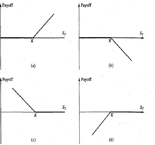
The value of an option at its expiry is usually called the payoff function. Let’s analyze now payoff of European options. As stated, a holder of European call/put option has the right to buy/sell (exercise) an underlying for strike price at expiration date. Whether the buyer will exercise option depends on price of asset at that date, i.e. if the price is higher/lower it will make profit to holder, therefore this

opportunity should be exploited. But if the price is lower/higher the investor will clearly choose not to exercise [Hull]. Therefore formula for the payoff of long position (holder) in a European call option is:

max(ST-K,0)

and payoff of long position in put,

max(K-ST,0).

Vice versa, for the writer of the option, that is short position in European call -max(K-ST,0)= min(K-ST,0)

and the payoff from a short position in European put option is -max(ST-K,0)= min(ST-K,0).

Here ST denotes price of asset at maturity, while K stands for strike price. Next figures illustrate payoff

Figure 1.1.1. Option payoff: a) long call b) short call c) long put d) short put

After all, it can be concluded that option must cost something, since one can make riskless profit by getting into long positions, also the writer of the option must be compensated for the obligation he has assumed [2]. In the next part is determined what should be the price of a European calls and puts.

1.3.

Arbitrage and risk free rate

Before modeling and finding the formula for option price, couple of fundamental concepts must be presented; these will be used as a tool for calculating option prices, and first one is arbitrage.

Definition: A portfolio is an arbitrage portfolio, if today it is of non-positive value, and in the future it has zero probability of being of negative value, and a non-zero probability of being of positive value [4]. In other words, there are never opportunities to make an investment to make instantaneous risk-free profit, at least such opportunity cannot exist for a significant length of time before prices move to eliminate them [2].

Other fundamental concept is assumption on existence of risk-free investment. This means that for the investment asset (or money) no risk of default by the counterpart exists. A good approximation of such are a government bonds, deposit in a bank with best credit rating or lately (after crisis) swaps. Portfolio invested in one of these gives back risk-free interest rate r.

1.4.

Modeling asset price

For the price to be found it should be modeled first. Efficient market hypothesis (EMH) considers that asset price follow stochastic process. It basically says that current price fully reflects past history, also it states that market responds immediately to any new information about the asset. Because of these assumptions, asset price is said to have Markov properties i.e. the probability distribution of the price at any particular future time is not dependent on the particular path followed by the price in the past.

Furthermore, it is usual to represent change in asset price using return𝑑𝑆 _𝑆, rather than absolute change. All of this brings us to most common model, geometric Brownian motion model for asset price movement.

𝑑𝑆

𝑆 = 𝜇𝑑𝑡 + 𝜎𝑑𝑋

The parameter 𝜇 is the expected rate of return on the asset and along with 𝑑𝑡 it represents

deterministic part of return, also called drift. It depends on the riskiness of the asset, as well as on level on interest rates in economy. In this thesis 𝜇 is taken to be constant, but in more complicated models, 𝜇 can be a function of S and t. Further, the variable 𝜎 is the volatility (𝜎2 is variance), and it is a measure of uncertainty about returns provided by the asset. It represents standard deviation of return, and it can be calculated in many ways. Finally, 𝑑𝑋 contains the information about the randomness of the asset price and is known as Wiener process or standard Brownian motion. 𝑑𝑋 is a random variable which follows a normal distribution, with mean zero and variance 𝑑𝑡, therefore 𝑑𝑋 can be written as

𝑑𝑋 = 𝜑 𝑑𝑡 [5]. Here 𝜑 is random variable with a standardized normal distribution. Its probability density function is given by

𝑓 𝜑 = 1

2𝜋𝑒

−1₂𝜑2_𝑑𝜑

,

for −∞ < 𝜑 < ∞. With the definition of expectation operator 𝜀 given by

𝜀[𝐹 ∙ ] = 1 2𝜋 𝐹 𝜑 ∞ −∞ 𝑒− 1 2𝜑2𝑑𝜑_, For any function F, we have

Further, it can easily be concluded, that if there is no uncertainty about the price (st.dev is 0)

𝑑𝑆 𝑆 = 𝜇𝑑𝑡

Integrating between time 0 and time T, we get

𝑆_𝑇 = 𝑆₀𝑒−𝜇𝑇

Where 𝑆0 and 𝑆𝑇 are the stock price at time 0 and time T. This equation illustrates that when there is no

uncertainty, the price grows at continuously compounded rate 𝜇 per unit of time [1], and it represents time value of money.

1.5.

The Black-Scholes-Merton Model

Black-Scholes-Merton model gives the partial differential equation which must be satisfied by the price of any derivative dependent on non-dividend asset. Starting point in derivation of the BSM equation is Ito’s lemma (more on lemma and its derivation in [4], [6] and [1]).

𝑑𝑓 = 𝜕𝑓 𝜕𝑆𝜇𝑆 + 𝜕𝑓 𝜕𝑡+ 1 2 𝜕2_𝑓 𝜕𝑆2𝜎2𝑆2 𝑑𝑡 + 𝜕𝑓 𝜕𝑆𝜎𝑆𝑑𝑋

Latest equation presents the random walk followed by 𝑓, where 𝑓 is the price of derivative which is affected by S and t.

Idea of Black-Scholes-Merton model is to create riskless portfolio, which means eliminating stochastic part in it. Therefore, return from that portfolio should equal to risk-free interest rate (r), in the absence of arbitrage argument. Risk-less portfolio in this case involve (short) position in the derivative and appropriate amount of underlying stock (asset). This can be done because both depend on the same source of uncertainty, i.e. stock price movements.

Finally, before BSM equations are derived, some assumptions must be made.

1. The stock price follows the process developed stochastic process with 𝜇, and 𝜎 constant. 2. The short selling of securities with full use of proceeds is permitted.

3. There are no transactions cost or taxes. All securities are perfectly divisible. 4. There are no dividends during the life of the derivative.

5. There are no riskless arbitrage opportunities. 6. Security trading is continuous.

7. The risk-free rate of interest, r, is constant and the same for all maturities. Now all the tools we need for deriving BSM equation are set [1].

Consider the situation when (as mentioned above) the holder of portfolio is short one derivative and long an amount 𝜕𝑓

𝜕𝑆 of shares with a goal to eliminate stochastic part. 𝛱 denotes the value of

portfolio

Π = −𝑓 +𝜕𝑓 𝜕𝑆𝑆

The change 𝑑Π in the value of portfolio value in the time interval 𝑑t is given by

𝑑Π = −𝑑𝑓 +𝜕𝑓 𝜕𝑆𝑑𝑆

(𝜕𝑓_𝜕𝑆 is held fixed during very short period of time). Substituting geometric Brownian motion equation and Ito’s lemma into later equation yields:

𝑑Π = (−𝜕𝑓 𝜕𝑡− 1 2 𝜕2_𝑓 𝜕𝑆2𝜎2𝑆2)𝑑𝑡

So stochastic part is eliminated, i.e. portfolio is risk-less therefore it should earn risk-free interest rate

𝑑Π = rΠ𝑑𝑡

Substituting equations for Π and 𝑑Π, we arrive at

𝜕𝑓 𝜕𝑡 + 1 2 𝜕2_𝑓 𝜕𝑆2𝜎2𝑆2 𝑑𝑡 = 𝑟(𝑓 − 𝜕𝑓 𝜕𝑆𝑆)𝑑𝑡.

We finally got Black-Scholes-Merton, which after sorting looks like this

𝜕𝑓 𝜕𝑡 + 𝑟𝑆 𝜕𝑓 𝜕𝑆+ 1 2𝜎2𝑆2 𝜕 2_𝑓 𝜕𝑆2 = 𝑟𝑓.

This is stochastic differential equation, and solving it requires boundaries which will be described in next section.

Under assumptions stated above and with appropriate boundaries this equation has analytical solution for European options (more on derivation in [1]):

𝑐 = 𝑆0𝑁 𝑑1 − 𝐾𝑆−𝑟𝑇𝑁(𝑑2)

where c stands for price for call, the formula for put (p) is:

𝑝 = 𝐾𝑆−𝑟𝑇_{𝑁 −𝑑} 2 − 𝑆0𝑁 −𝑑1 where 𝑑1 = ln 𝑆0 𝐾 + 𝑟 +𝜎 2 2 𝑇 𝜎 𝑇

𝑑₂=ln 𝑆₀ 𝐾 + 𝑟 −𝜎 2 2 𝑇 𝜎 𝑇 = 𝑑1− 𝜎 𝑇

The N(X) is the cumulative probability distribution function for standardized normal distribution.

1.6.

Boundaries

Bounds are important for finding solution for every differential equation whether it will be

calculated numerically or analytically. First boundary is the most obvious one; the call option cannot be worth more than stock at current time, it stands for both American and European

Call ≤ S(0)

This is upper bound and if this was not true, the opportunity for arbitrage would exist, i.e. one could buy stock and sell the call option to obtain riskless profit. Lower bound for European call is

c ≥ S(0)-Ke-rT

Otherwise arbitrageur could buy an option and short the stock, with difference deposited at rate r. For European put option following is valid,

Max(Ke-rT-S(0),0) ≤ p ≤ Ke-rT

If left side of equation was different arbitrageur could buy put and take long position in stock (by borrowing money at rate r) to make profit. If the right side was not true profit would be made by selling put, and investing it at riskless rate r, then if option is exercised writer of the option would surely have more than enough money to buy an asset for K.

Bounds on American put option;

Max(K-S(0),0) ≤ P ≤ K.

Similar arbitrage opportunities as described are cause for these bounds. What would be the lower boundary for American call option? It would be

C ≥ S(0)-K

So the option is always greater than its intrinsic value for sure. Meaning of this is that American call option should never be exercised before expiration date. Intuition suggests that American option should be more valuable than European since it has all the same opportunities as European and some more,

and it true is for put. But because American call obviously doesn’t provide more opportunities than European, it must have the same value as European call.

1.7.

Who uses options and some exotic options

There are many different reasons to participate in the markets, but a broad classification of participants can be made according to their attitudes towards risk [4].

- The hedgers use market instruments to reduce risks. Usually companies use derivatives to reduce risk of buying or selling commodities at unfavorable prices.

- The speculator uses market instruments to increase his risk, meaning earning more profit. Using options speculator makes leverage in order to increase gains.

- The arbitrageur tries to spot discrepancies in the pricing of instruments (derivatives, stocks…). When spotted one can make riskless profit by buying at lower price and selling at larger, or similar.

Now some more derivative types, called exotic options will be introduced.

- Bermudan options – nonstandard American options with early exercise restricted to certain dates

- Barrier options – the payoff depends in whether the underlying asset’s price reaches a certain level during a certain period of time (down-and-in/out, up-and-in/out, knock-in/out…)

- Lookback options – price depends on the maximum or minimum reached during option’s life - Asian options – payoff depends in the arithmetic average of the underlying asset’s price during

the life the option

There are many other options available on the market, but these are introduced because they are going to be mentioned in thesis.

2.

Numerical methods for option pricing

2.1.

Binomial tree

The first numerical procedure for option pricing which will be analyzed is binomial tree, it is one of the simplest and most widely used methods. Particularly the Cox, Ross, Rubinstein (CRR) [7]tree is going to be used in this thesis. The CRR binomial tree is a discrete version of the Black-Scholes constant volatility process. Every numerical solution is just an approximation of the price, the aim here is to find how it behaves, and how to obtain the most precise and the fastest solution.

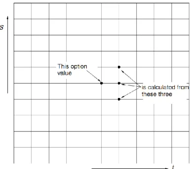
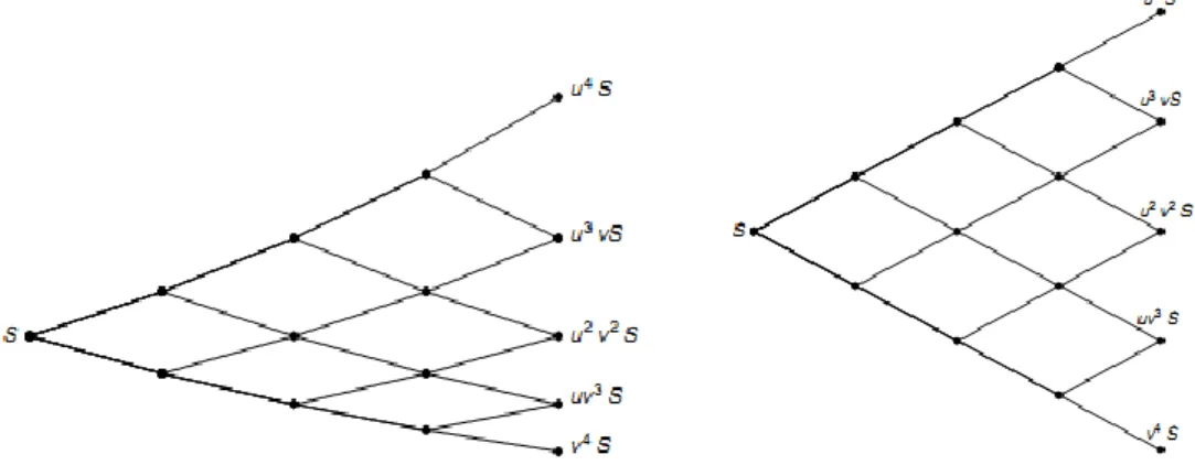
Binomial pricing model arises from discrete random walk models of the underlying asset. The idea is to break down the time to expiration into potentially very large number (N) of time intervals, or steps (0, dt, 2dt…ndt where n is natural number n≤N) . First step is to initial the tree of stock prices by moving forward from present to expiration. At each step it is assumed that the stock price will move up (by the factor u) or down (factor u).

Figure 2.1.1. Graphical representation of binomial tree

One should find a way to calibrate the lattice so that it reflects the underlying model which is a continuous-time, continuous-state stochastic differential equation [8]. Following this model, no-arbitrage and risk neutral principles crucial parameters are obtained (derivation in [1] and [2]).

Risk-neutrality demands: 𝑆𝑒𝑟 𝑑𝑡 = 𝑝𝑆𝑢 + 1 − 𝑝 𝑆𝑑, that is 𝑒𝑟 𝑑𝑡 = 𝑝𝑢 + 1 − 𝑝 𝑑, 𝑝 is probability of an up movement, and since it is binomial tree (1-p) is the probability of a down movement. Equation reflects that discounted expected return equals current price.

Using condition introduced by Cox, Ross, Rubbenstein:

𝑢 =1 𝑑

Following are obtained:

𝑝 =𝑒𝑡𝑑𝑡 − 𝑑 𝑢 − 𝑑 𝑢 = 𝑒𝜎 𝑑𝑡

𝑑 = 𝑒−𝜎 𝑑𝑡_.

From figures and equations, it can be concluded that tree recombines so that in every time step we have in ith step i+1 prices (some are recombined, i=0...N), totaling (N+1)(N+2)/2 nodes (lattices) in tree of N steps. Also there are 2N+1 different possible price (this will be useful later). Furthermore, as price at time zero is known (S0) , all feasible prices are obtained using

𝑆₀𝑢𝑗_𝑑𝑖−𝑗 _{or 𝑆} 0𝑢2𝑗 −𝑖

Since 𝑢 =_𝑑1.

Having the tree of stock prices constructed, and with all parameters, it can be derived how to get the price of particular option, working backward in the tree. At the end step of the tree, i.e. at expiration of the option, the option values for each possible stock price are known, as they are equal to their intrinsic values. Assuming that the pay-off function of the option is determined only by the value of the underlying asset at expiration, the model then works backwards through each time interval,

calculating the option value at each step. The final step is at current time and stock price, where the theoretical fair value of the option is calculated. Algebraically it means for call option:

𝑓_𝑁,𝑗 = max 𝑆₀𝑢𝑗_𝑑𝑁−𝑗 _{− 𝐾, 0 , 𝑗 = 0,1, … , 𝑁}

And for put option

𝑓_𝑁,𝑗 = max 𝐾 − 𝑆₀𝑢𝑗_𝑑𝑁−𝑗_{, 0 , 𝑗 = 0,1, … , 𝑁.}

Followed by working backward trough the tree

𝑓_𝑖,𝑗 = e−rdt _𝑝𝑓

𝑖+1,𝑗 +1+ (1 − 𝑝)𝑓𝑖+1,𝑗 , 𝑗 = 0,1, … , 𝑁.

and j denotes lattice position in i-th step of the tree, so it can take values up to i.

The main reason for introducing Binomial tree was inability to calculate the price of an American style option using BSM equation. So, following equations are taking into account early exercise possibility in American calls and puts:

𝑓_𝑁,𝑗 = max 𝑆₀𝑢𝑗_𝑑𝑁−𝑗 _{− 𝐾, e}−rdt _𝑝𝑓

𝑖+1,𝑗 +1+ (1 − 𝑝)𝑓𝑖+1,𝑗

𝑓_𝑁,𝑗 = max 𝐾 − 𝑆₀𝑢𝑗_𝑑𝑁−𝑗_{, e}−rdt _𝑝𝑓

2.1.1. Implementation and results

Binomial tree is pretty much strait forward for implementation. Custom made functions (some based on [8]) are done in MatLab:

Functions

- Eur.m – direct tree implementation from Hull’s book, , returns both call and put - EurSmart.m – more efficient implementation (description follows)

- AmPut.m – similar to Eur.m just for American puts - AmPutSmart.m – similar to EurSmart

Main programs

- ProgramEu – requires inputs, returns comparison plot of time required for Eur.m and EurSmart.m for different number of steps used in tree, also calculates BSM both put and call prices using analytical solution, as well as doing it numerically (averaging prices for N and N-1) - ProgramAm – does the similar as ProgramEu.m, with addition of calculating American put

option using control variate technique.

In next figure and table some example results are presented for American put option.

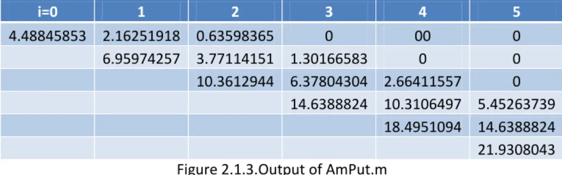
Figure 2.1.2.Binomial tree for American option as an output of DerivaGem – Version 2.01 in Excel, J.C.Hull [1]

i=0 1 2 3 4 5 4.48845853 2.16251918 0.63598365 0 00 0 6.95974257 3.77114151 1.30166583 0 0 10.3612944 6.37804304 2.66411557 0 14.6388824 10.3106497 5.45263739 18.4951094 14.6388824 21.9308043 Figure 2.1.3.Output of AmPut.m

AmPut.m can return list of matrix elements where early exercise occurred.

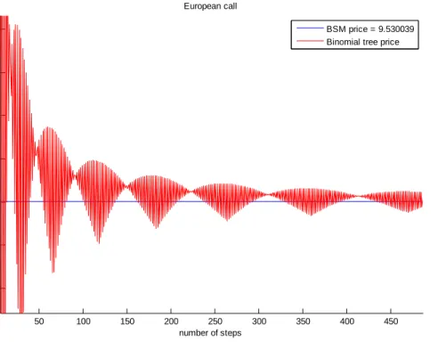
Now the behavior of Eur.m is analyzed and compared to MatLab internal function blsprice.m, on an example with same parameters as before on European call option (S(0)=50, vol=0.4, r=0.1, T=5/12, K=50). It is direct application of simplest algorithm for binomial tree described in Hull. From the figure it can be noticed that binomial tree is not good at all at beginning (small number of steps used), but it converges to the right price in every step (or every few steps).

Figure 2.1.4.Convergence of Binomial tree with increase in Number of steps

blsprice 500 1000 1500 2000 2500 3000

time (s) 0.3132498 0.027121 0.079032 0.174457 0.312989 0.469533 0.683818 price 6.1165081 6.1139620 6.1152349 6.1156593 6.1158715 6.115999 6.116084 error 0 -0.0025461 -0.0012732 -0.0008488 -0.0006366 -0.00051 -0.00042

Table 2.1.1. European option time and resulting price using binomial tree

0 5 10 15 20 25 30 35 40 45 50 5.4 5.6 5.8 6 6.2 6.4 6.6 6.8 7 7.2 7.4 number of steps p ri c e BSM price Binomial tree price

All measurements from now on, except when it is stated otherwise are done on Lenovo G560 Laptop (Intel Celeron T3500 (2 cores 2.1GHz), 2GB DDR2 RAM) in Windows 7 environment.

Although it successfully provides decent approximation, there are few downsides of binomial tree implemented as in Eur.m and AmPut.m. As traders require really precise value of option the drawback of binomial tree is that it converges very slow to BSM price, when using 3000 steps

measurement uncertainty is ~0.00042 in this case (which can be a lot of money, considering the huge possible amounts of trades). Furthermore there is a memory issue, which means that N can’t be taken as large as we want since the algorithm is using matrix of (N+1)x(N+1). On tested computer and MatLab version maximum N is 6938, which is not enough in many cases. Finally, at N=500 lattice method is significantly faster than blsprice but increasing number of steps computational price rises, logically, at rate of ~n^2 (where n is factor of increase in steps).

2.1.5.Possible scheme for storing prices

If having the whole tree in the memory is not required, and it isn’t in most of the cases, algorithm can be improved. It can be noticed that only one vector of length 2xN+1 can be used for storing all the possible stock prices (ud=1, as already explained tree recombines), instead of matrix. This is illustrated in the figure 2.1.5. It can be noticed that odd numbered lattices correspond to the last time layer, whereas even numbered entries correspond to the second to last time layer, and so on. So the algorithm function in the following manner: first put all payoffs at odd numbered places in vector, then continue computing as in first algorithm with difference that everything is stored in one vector,

alternating between using odd and even places in vector, until finally option price is calculated. Its position is N+1 in vector.

Figure 2.1.6.Convergence with the same parameters only stock price is changed S(0)=55 ( N=500 for illustration)

Using binomial tree price of the option can be determined with a precision that we need, it is just question of computational time. The “smart” functions which use improved algorithm are usually much faster than original algorithm, furthermore they are far more memory efficient providing us with a possibility of using many more steps to obtain more precise value (the time can be even more decreased if in function only one price is calculated put or call not the both).

Moreover, in order to improve the precision and memory usage of the algorithm, intuition may suggest finding some kind of an average of the couple of last prices. Looking at plot in figure 2.1.4 it seems that it would give value which is really close to BSM price, and it would, but only in this case when exercise and stock price are same. With different parameters convergence is more likely to look like one on figure 2.1.6. So it cannot be done with just averaging few values, although it provides somehow better results. Some other techniques can be used (just use smaller value of two consecutive numbers of steps, or use low pass filters, moving-average…).

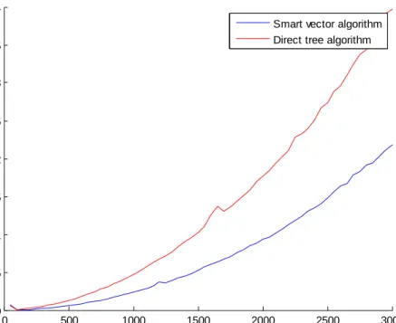
Figures 2.1.7. and 2.1.8. compare the speed of two algorithms. For European option “smart” algorithm is approximately two times faster as can be seen from table 2.1.1. too. On figure for American option first can be noticed that direct implementation with tree is much slower than smart, while times for improved algorithms are similar to those in European smart.

50 100 150 200 250 300 350 400 450 9.51 9.52 9.53 9.54 9.55 9.56 9.57 number of steps p ri c e European call BSM price = 9.530039 Binomial tree price

Figure 2.1.7.Speed Comparison: EurSmart.m and EurPut

Figure 2.1.8.Speed Comparison: AmPutSmart.m and AmPut

S(0)=48; K=50; r=0.1; vol=0.2; T=0.5; N=3000; yields price for American option 2.927356

0 500 1000 1500 2000 2500 3000 0 0.05 0.1 0.15 0.2 0.25 0.3 0.35 0.4 number of steps ti m e [ s ]

Smart vector algorithm Direct tree algorithm

0 500 1000 1500 2000 2500 3000 0 0.5 1 1.5 number of steps ti m e [ s ]

Smart vector algorithm Direct tree algorithm

2.1.1.1. AMERICAN OPTION CONTROL VARIATE TECHNIQUE

CRR method’s greatest advantage is that it can easily handle pricing of American options. There are techniques which improves CRR performance when dealing with early exercise. Accuracy and therefore speed of binomial tree technique can be improved by using control variate technique. It involves using same the number of steps and same parameters (and therefore using the same tree), for both American and European option. As exact solution using BSM exists, meaning that error can be calculated for CRR European style option. Moreover, it is assumed that it equals the error of American option, so price of American option can be approximated [1].

To put it to test author used the same parameters as in 2.1.1. and with S(0)=55. Results are following: Price of American option using AmPutSmart: 2.595617

Prices for European put using BSM, CRR and their difference: BSM= 2.489511

CRR = 2.490316 (N=300) dif= -0.000805

Control variate technique therefore gives: 2.594812

Price for American option using 30001 time steps: 2.594661 European: (large 2.489548) It was tested with similar results with other values and number steps. Control variate technique obviously reduces error, so finally one can say that American option price can be approximate with decent precision using binomial tree and control variate technique.

2.1.2. Conclusion

In this chapter the basics of the binomial model were described. Also, pricing equations and algorithms were derived for both European and American-style exercise. The method can be extended in many ways, to incorporate dividends, to allow Bermudan exercise, to value path-dependent contracts and to price contracts depending on other stochastic variables such as interest rates. The main

advantage of binomial trees is easiness of implementation and it is easy to understand it. The author has not gone into the method in any detail for the simple reason that the binomial methods just a simple version of an explicit finite-difference scheme. As such it will be discussed in FDM chapter, which are far more flexible [9].

2.2.

Monte-Carlo

Monte Carlo simulation is an important tool in computational finance, in fact for many applications it is the only way to price a derivative. Starting point for constructing simulation is, again, stochastic differential equation based on Brownian motion. If we recall from introduction, the fair option value in the Black-Scholes world is the present value of the expected payoff at expiry under a risk-neutral random walk for underlying [9]

Using two facts mentioned above Monte Carlo simulation for option pricing is based on following simple steps:

- Generate path of stock price using random walk model in risk-neutral world - Get payoff

- Perform many more such realization over time horizon

- Calculate average payoff for all realization to get expected payoff - Present value of this average payoff is an approximation of option price Paths are generated using:

𝑑𝑆 = 𝑟𝑆𝑑𝑡 + 𝜎𝑆𝜑 𝑑𝑡

This discrete way of simulating the time series for stock price is called Euler method. It implies that change in price can be calculated from previous step price.

Moreover, for lognormal random walk there is simple, and exact, time stepping algorithm. Ito’s lemma leads to:

𝑑 𝑙𝑛𝑆 = 𝑟 −1

2𝜎2 𝑑𝑡 + 𝜎𝜑 𝑑𝑡

which after integrating provides:

𝑆(𝑡 + 𝑑𝑡) = 𝑆 𝑡 exp⁡( 𝑟 −1₂𝜎2 _{𝑑𝑡 + 𝜎𝜑 𝑑𝑡). (2.2.1)}

What is important here is that there is no need for dt to be small as formula is exact, thus it is the best time stepping algorithm to use. Also, if one is not interested in path of the option, payoff can be directly calculated by taking T as a time step.

One possible GBM path created using derived formulas for N time steps

As for measurement uncertainty, Euler’s approach has an error of 𝑂(𝑑𝑡) (although better approximation exist, e.g. the Milstein method which has an error of 𝑂(𝑑𝑡2)). To illustrate without proving it, take dt as time step for some path dependent options, e.g. barrier option. There is a possibility of missing the barrier being triggered between steps [9]. So it can be interpreted that the error which comes from the finiteness of the time step is 𝑂(𝑑𝑡).

Furthermore, consequence that only limited number of paths can be produced is error which equals 𝑂(𝑁−

1

2)_{, where N is number of paths. So the total error is the worst error of two} 𝑂(𝑑𝑡) _and

𝑂(𝑁−12)_{. To minimize this, it is required to keep} 𝑁 = 𝑂(𝐾 2

3) _and 𝑑𝑡 = 𝑂(𝑁− 1

3)_{, where} 𝐾 = 𝑂(𝑁

𝑑𝑡) [9].

Therefore to increase precision by factor of X, number of simulations must be increased X2 times. One of the greatest advantages of MC is that it can handle European-style options that depend on many variables. Indeed, PDEs with d+1 (d number of dependent assets) variable can be written, but it would be very time consuming to compute, even comparing to MC. Equation for many variables is basically the same except 𝜑𝑖 which is correlated

𝑆_𝑖(𝑡 + 𝑑𝑡) = 𝑆_𝑖 𝑡 exp⁡( 𝑟 −1₂𝜎_𝑖2 _{𝑑𝑡 + 𝜎}

𝑖𝜑𝑖 𝑑𝑡).

Correlated random variables are calculated using Cholesky decomposition (procedure is explained in [9]). 0 0.05 0.1 0.15 0.2 0.25 0.3 0.35 0.4 0.45 0.5 40 45 50 55 60 65

2.2.1. Implementation and results

In this section, few different sequential implementations for Monte Carlo option pricing for vanilla options will be analyzed, it will be followed by parallel implementation with results and analysis. Finally next section is devoted to American up option.

2.2.1.1. Sequential implementation

Codes used for implementation and testing are:

- MCdt.cm – generate N option paths with n+1 time steps, applying directly formula (2.2.1) using

for loops

- MCvectorized.m – does the same as first two codes, only in the vectorized form which is far more suitable for Matlab, without for loops (furthermore it saves all paths in matrix);

- MC1.m – generate N prices at T applying (2.2.1.) with for loops (using only one time step of size T, and loosing information about paths)

- MC1vec.m – same as MC1.m in vectorized form - MC.c – same as MC1.m, only it is in C

All are for European call option.

Used parameter: S(0)=50, K=50, r=0.05, vol=0.3; T=0.5 with different N and n.

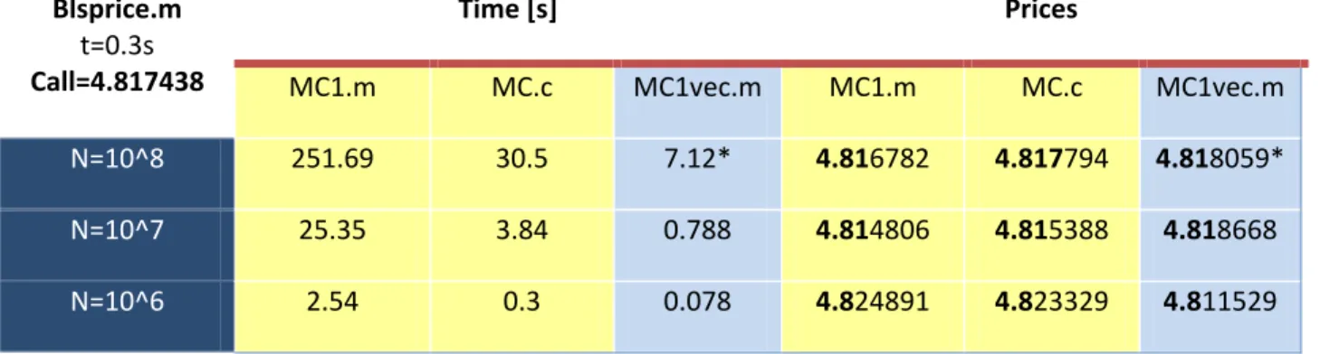
Blsprice.m t=0.3s Call=4.817438 Time [s] Prices MC1.m MC.c MC1vec.m MC1.m MC.c MC1vec.m N=10^8 251.69 30.5 7.12* 4.816782 4.817794 4.818059* N=10^7 25.35 3.84 0.788 4.814806 4.815388 4.818668 N=10^6 2.54 0.3 0.078 4.824891 4.823329 4.811529

Table 2.2.1.: results for MC1.m, MC.c, MC1vec.m * for loop used because N reached limit

In table 2.2.1., functions which doesn’t calculate whole paths are compared (dt=T, n=1).It can be noticed that the same algorithm applied in C is more than 8 times faster than MatLab version. But MatLab deals with matrices/vectors better, so the vectorized MatLab code is ~4 times faster than algorithm in C. Also table shows (in prices part) how accuracy increases with more paths simulated. This is consistent with mentioned error 𝑂(𝑁−

1

only useful for calculating European option, and it can be used as a foundation for the future development.

code for vectorized implementation

Values_at_T=S*exp((r-0.5*vol^2)*T + vol*sqrt(T)*randn(N,1)); option_values=max(final_vals-K,0);

present_vals=exp(-r*T)*option_values; price=mean(present_vals);

Now somewhat more useful algorithms are compared, i.e. simulating whole path of stock price Blsprice.m t=0.3s Call=4.817438 Time [s] Prices MCdt.m MCvectorized.m MCdt.m MCvectorized.m N=10^5, n=173 123.9 1.25 4.8212 4.8225 N=10^6, n=20 143.2 1.47 4.8111 4.8215 N=10^7, n=1 100 1.1 4.8165 4.8164 100x N=10^5,n=173 * 13118 123 4.8156 4.8179 Table 2.2.2.

Again it can be seen that MatLab simulation using matrices, without loops is much faster than version with loops, in fact it is approximately 100 times faster. The difference is even greater when MCdt.m saves the paths. Advantage of MCvectorized.m against all the other MCs so far is that it stores paths in matrix, and one can now calculate American options, or any of the Exotic options. When the code produces paths but doesn’t save them, not all kind of options can be valued (e.g. American using Longstaff Schwarz method). Vectorized version though has one flaw, it requires a lot of memory so first three cases are near the maximum use of memory (on author’s Lenovo laptop).Third case is basically the same as 2nd case in table 2.2.1, but due different implementation it is slower, although not that drastic. Further, 4th example is useless in the sense of saving paths of the options, and it is presented in order to compare it MC1s results. In fact, both third and fourth examples converge to the right value at the same pace, and it doesn’t matter if many or just one step is used. This is implied by equation 2.2.1.

Code for vectorized, paths are stored in SPaths

Product=exp(nudt+sidt*randn(NPaths,NSteps)); SPaths=cumprod([S0*ones(NPaths,1),Product], 2); option_values=max(SPaths(:,NSteps+1)-K,0); price=mean(option_values)*dicount;

2.2.1.2. Parallel implementation

Obviously there is a need for improving speed simulation, since it is common to calculate many prices as well as Greeks and other parameters. In this thesis idea is to improve the speed of Monte-Carlo by using more processors. For this purpose triqui3.fi.upm.es was used (Dell Poweredge 2950 Dual 3 GHz Quad Core Intel Xeon , memory: 16GB per node: operating system: CenTOS 5.5, Linux installed).

Algorithm for parallel implementation is basically the same as MC1.m and MC.c with that difference that calculation are divided to more processors using MPI. Also since it is implementation in C, there is a need for generating numbers from normal distribution, for that purpose Box-Muller method is used, with all its flaws.

Pseudo code for multi-processor implementation of Monte-Carlo (mcMPI1.c)

// rank of master is 0, and there is N processors so N-1 is the maximum rank

If rank=master

//send the jobs to the slaves, i.e. 1...N-1

{

For (rank=1..N-1)

// evenly divided number of total number of simulation are sent to each processor

Send(n/N, rank) EndFor

// after sending the work master continue to do the same simulation as slaves

For (i=1..n/N ) SimulatePath

Payoff(i)=max(SimulatedPayoff,0) endFor

//master calculated price is stored in Price(0)

Price(0)=discount*average(SimPay)

// receive prices values from slaves, store it appropriately, and send end tag to processors

For (rank=1..N-1) Receive(result, rank) Price(rank)=discount*result Send(end_tag, source.rank) endFor } // Slaves Else {

//receive number of simulations assigned/ check if tag is for ending

Receive(n/N, tag) If tag==end_tag{

Break} Else

// do the simulations, calculate prices, and send results to master

SimulatePath Payoff(i)=max(SimulatedPayoff,0); endFor Result=discount*average(SimPay) Send(result, 0) endIfElse }

// calculate average of prices received by all processors

Price=sum(price(0…N-1))/N End

Of course, this can be done differently using MPI_REDUCE or similar but above algorithm yields result which cannot be much better in this kind of implementation. Only drawback that may arise here is, if some processors are already used by another activity, the processor with greatest load will do required job slower and whole computational time will depend on slowest processor. This can be noticeable when working with more than 10^8 simulations. During testing usually processors finished in more or less same time (+-2.5%). So load of processors was the same. If different implementation was tried, worse times can occur because of communication time between the processors. So if other method is used attention must be devoted to minimize communication and maximize productivity.

Other than mcMPI1.c two more were used:

- mc.c – sequential implementation as in section 2.2.1.2 with MPI used just for timing - mcMPIat.c – uses antithetic variables to speed up convergence

Antithetic variate technique deserves explanation. The method uses two estimates for an option value which are calculated using same set of random numbers. With that set, one approximation of future price is made and using the same random numbers only with minus sign the other estimate is simulated. Having two estimates prices are calculated in usual way find payoff and discount it. Final approximation using antithetic variables is the average of two estimates using same random set. Of course, since it is still Monte Carlo simulation this operation should be repeated many times to get an accurate estimate for the option value. This technique works because of the symmetry in the Normal distribution. This symmetry is guaranteed by the use of the antithetic variable [9].

Confidence intervals for plain MC vs. Antithetic [20]

BSM price Call=4.817438

Time [s] Prices

mc.c mcMPI1.c mcMPIat.c* mc.c mcMPI1.c mcMPIat.c*

N=10^6 0.17 0.046 0.056 4.816812 4.809594 4.815486 4.804397 4.813292 4.80555 4.817293 4.816741 4.817987 10^7 1.67 0.40 0.48 4.820400 4.814978 4.820495 4.818605 4.82055 4.817352 4.817955 4.818307 4.817889 10^8 16.82 3.96 4.8 4.818611 4.817711 4.816211 4.817608 4.818232 4.817855 4.817424 4.818229 4.817792 10^9 170.3 41.32 48.35 4.817173 4.817512 4.817471 4.817925 4.817566 4.817538 4.817732 4.817593 4.817248 Table 2.2.3. Comparison of price values and computational time for sequential, parallel and

antithetic parallel algorithm

* mcMPIat – uses basically 2xN paths for evaluation, but since computational time increases only by ~20% with that number of paths it is included in this table

BSM price

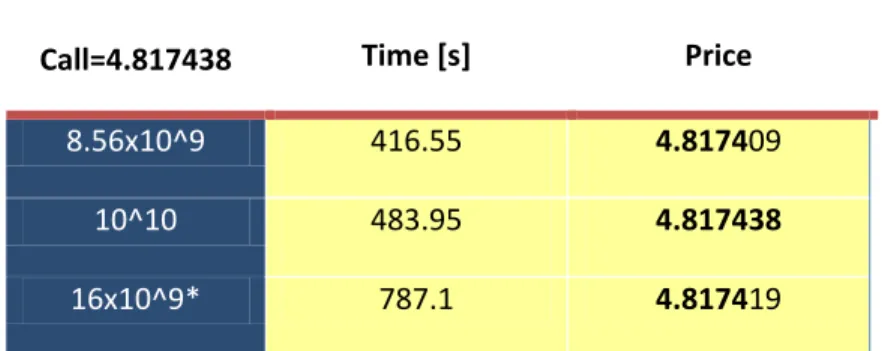
Call=4.817438 Time [s] Price 8.56x10^9 416.55 4.817409

10^10 483.95 4.817438 16x10^9* 787.1 4.817419

Table 2.2.4. Output of antithetic parallel implementation for larger number of simulations with a goal to get the most accurate results using MC in this thesis

* 3rd case is using near max unsigned long int, for maximum precision (loop can be added for whole function and evade max unsigned long int), in fact it uses 4(processors) x 4e9 (~max unsigned int) x 2 (antithetic)=32e9 different paths.

2.2.2. American options Longstaff Schwartz method - algorithm and results

As stated before, valuation of derivative with early exercise feature is the major challenge in the field. Monte Carlo simulation is generally considered as not particularly well suited for valuing American options. In this section Longstaff Schwarz [10] method is presented. It is one of the simplest methods to implement, since only least squares are required to find appropriate value. Yet, method is powerful and can be applied to derivatives with both path-dependent and American-exercise features. Also, LSM allows variables to follow stochastic processes such as jump diffusions so it can be very general. Method will be described now. In LSM once again we go backwards, that is first step is to calculate cash flows at received at expiration date. Then in every step check for every path if it is in the money, if so we it should be decided whether it is good time to exercise. To estimate the expected cash flow from continuing the option’s life conditional on the stock price at time which is currently observed discounted continuation values from previous step (i+1) are regressed to current (i). It is done in following way using least square. First calculate coefficients a,b,c by minimizing:

(𝑉𝑘− 𝑎 − 𝑏𝑆𝑘− 𝑐𝑆𝑘2)2 𝑛

𝑘=1 (2.2.2.1)

Here, k represents one of the in the money paths, and n is total number of paths with positive payoff at current time-step. S represents stock price at current time step, and V is discounted value of continuing discounted to current step. When coefficients are calculated then continuing values for current time step can be found using.

These values are compared to the value of exercising option, and if the option should be exercised its exercise value is taken into account in cash flows. Proceeding recursively backwards next time step is evaluated, and so on until present time is reached. Only, the realized discounted cash flows are used for previous step (in first step payoffs). The value of the option is determined by discounting each cashflow back to time zero, and calculating mean of the results.

Comment: In LSM if at node option is out of the money it doesn’t matter what the continuation value is since it is easier to accurately fit on a smaller domain, so only in-the-money are taken into account. On the other hand Glasserman [11] recommends using out-of-the money options as well.

2.2.2.1. Implementation and results

Algorithm is implemented in LSM_American.m, parameters used for testing are: S(0)=55, K=50, r=0.1, vol=0.3, T=1 and binomial tree with 3000 steps using control variate technique gives price 2.604429, while LSM method with 173 time steps and 10^5 paths outputs 2.601976, which is a decent

approximation for 10^5 path. Although, it must be emphasized that LSM MC can produce better and worse approximation than this one since it is stochastic

2.2.3. Conclusions

Monte Carlo is often used because of the following advantages: - Mathematics is usually very basic

- Path dependent options are easily incorporated - It is widely used for options affected by more variables - Correlations are easily modeled

- To get better accuracy simply run more simulations And drawbacks are:

- Computational cost - not so easy pricing of American options

2.3.

FDM

Finite difference methods (FDMs) is the generic term for a large number of procedures that can be used for solving a (partial) differential equation, which have as a common denominator some

discretization scheme that approximates the required derivatives [12]. FDM cope very well with rather smaller number of dimensions. Here, techniques that suits best BSM PDE will be introduced and implemented.

Idea in finite difference method is to find solution for differential equation by approximating every partial derivative numerically. After solution is found, it can be applied to a grid, which will be also explained.

For a given function f derivative in discrete form is defined by:

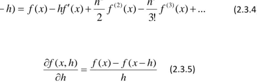
h x f h x f h h x f( , ) _ (  ) ( )   (2.3.1)

h in this case represents differentiation step and it is finite. As it can be guessed this formula is not accurate. Above formula is derived from Taylor series for 𝑓(𝑥 + ℎ) about (x,h):

...

)

(

!

3

)

(

2

)

(

)

(

)

(















h

f

x

h

f

x

h

f

x

h

f

x

x

f

Subtract f(x) from both sides and divide by h and there is exact representation of first equation:

)

(

)

(

...

)

(

!

3

)

(

2

)

(

)

,

(

h

O

x

f

x

f

h

x

f

h

x

f

h

h

x

f





















As it can be seen error is O(h), in this case. This approximation is called forward difference, using the similar Taylor series for 𝑓(𝑥 − ℎ) backward difference is obtained, with same error

...

)

(

!

3

)

(

2

)

(

)

(

)

(















h

f

x

h

f

x

h

f

x

h

f

x

x

f

Subtracting (2.3.4) from (2.3.2), and dividing it with 2h, gives the best approximation so far, the central difference. Following expression for derivative has an error O(h2).

) ( ) ( ... ) ( ! 5 ) ( ! 3 ) ( 2 ) ( ) ( ) , ( (5) 2 4 ) 3 ( 2 h O x f x f h x f h x f h h x f h x f h h x f _    _{       }   (2.3.5) Finally, approximation for second derivative is obtained by adding (2.3.4) and (2.3.2), and dividing with h2. Following expression has an error O(h2).

... ) ( ! 6 2 ) ( 12 ) ( ) ( ) ( 2 ) ( ) , ( (6) 4 ) 4 ( 2 ) 2 ( 2 2 2            x f h x f h x f h h x f x f h x f h h x f

Obviously error is O(h2). Of, course, by using more surrounding elements even more precise value of derivative can be achieved, but techniques that are presented here don’t demand it. Depending on which combination of presented schemes for derivatives is used in discretization of BSM equation, one can end up with different approaches, explicit, implicit or Crank-Nicolson.

Figure 2.3.1. Graphical representation of first order derivative using backward, forward and central difference

Now, when the approximation of derivatives is introduced, there is a need for grid. How is the grid for FDM made? First, for every differential equation solution space must be bounded, it is done basically using boundaries from first chapter. So, terminal condition is

𝑓_𝑖,𝑁 = max 𝑖𝑑𝑆 − 𝐾, 0 , 𝑖 = 0. . . 𝑀

For call, and for put

𝑓_𝑖,𝑁 = max⁡(𝐾 − 𝑖𝑑𝑆, 0).

Furthermore, S is bounded at S=0, and it is always 𝑓_0,𝑗 = 0 for call option, and for call option

𝑓0,𝑗 = 𝐾𝑒−𝑟(𝑁−𝑗 )𝑑𝑡, 𝑗 = 0. . . 𝑁

The fact that S is not bounded on upper side, one can overcome by taking S large enough. Upper

boundary in practice does not have to be too large. Typically it should be three or four times the value of the exercise price (or some other important price) [9]. So, for call

𝑓_𝑀,𝑗 = 𝑀𝑑𝑠 − 𝐾𝑒−𝑟 𝑁−𝑗 𝑑𝑡

and, obviously for put

𝑓𝑀,𝑗 = 0.

Bounds for American put

𝑓_0,𝑗 = 𝐾

𝑓𝑖,𝑁 = max⁡(𝐾 − 𝑖𝑑𝑆, 0)

𝑓_𝑀,𝑗 = 0

From (S,t ) continuous space, discrete one is made by dividing time from 0 to T (expiration date) in N steps of size dt, as well as dividing price axis in M number steps dS. So grid consists of points (S,t) such that 𝑆 = 0, 𝑑𝑆, 2𝑑𝑆, … , 𝑀𝑑𝑡 ≡ 𝑆_𝑚𝑎𝑥 and 𝑡 = 0, 𝑑𝑡, 2𝜕𝑡, … , 𝑁𝑑𝑡 ≡ 𝑇 [8]. In this thesis both will be divided in equal steps, although it is not the case always.

Having the grid, and numerical solutions for derivatives it will be continued to finite difference method, in usual order, first the solution for European style option is derived and implemented, then for American.

2.3.1. Explicit FDM

By using central difference with respect to stock price S, and backward difference to approximate time (t), the explicit method is derived. [8]

𝑓_𝑖,𝑗 − 𝑓_{𝑖,𝑗 −1} 𝜕𝑡 + 𝑟𝑖𝜕𝑆 𝑓_𝑖+1,𝑗 − 𝑓_{𝑖−1,𝑗} 2𝜕𝑆 + 1 2𝜎2𝑖2𝜕𝑆2 𝑓_𝑖+1,𝑗 − 2𝑓_𝑖,𝑗 + 𝑓_{𝑖−1,𝑗} 𝜕𝑆2 = 𝑟𝑓𝑖,𝑗

Rewriting the equations gives,

𝑓_{𝑖,𝑗 −1}= 𝑎_𝑖∗_𝑓 𝑖−1,𝑗 + 𝑏𝑖∗𝑓𝑖,𝑗 + 𝑐𝑖∗𝑓𝑖+1,𝑗, 𝑗 = 𝑁, 𝑁 − 1, … ,1,0; 𝑖 = 1,2, … , 𝑀 − 1, Where 𝑎_𝑖∗₌1 2𝜕𝑡(𝜎2𝑖2− 𝑟𝑖) 𝑏_𝑖∗_{= 1 − 𝜕𝑡(𝜎}2_𝑖2_{+ 𝑟𝑖)} 𝑐_𝑖∗₌1 2𝜕𝑡(𝜎2𝑖2+ 𝑟𝑖)

Figure 2.3.1.1.The relationship between option values in the explicit method.

Since the payoff, i.e. the prices at j=N are known, M-1 options values in N-1-th step can be calculated easily using derived expression, other two values (at i=0 and i=N) are known from boundaries. Therefore the same calculation continues until grid is completely filled. After every time step it can be easily checked if there is possibility for early exercise for American option by comparing obtained price with intrinsic value at that point (similarly to CRR). When the step for the present time is calculated, option price can be read from received values if we have it for required stock price. If that is not the case, value is interpolated using some kind of interpolation (cubic spline, linear, …).

Explicit method looks just fine, but still it has one major disadvantage, the stability issue. Namely, it can be proved that if 0 <_𝑑𝑆𝑑𝑡2≤

1

improved by halving the stock price step, time step must be reduced by a factor of four or more. The computation time then goes up by a factor of eight. The improvement in accuracy we would get from such a reduction in step sizes is a factor of four since the explicit finite-difference method is accurate to O(δt,δS2) [9].

2.3.2. Implicit FDM

To overcome the issue of stability, implicit method is introduced. The only difference in deriving implicit FDM is that for 𝑑𝑓

𝑑𝑡 backward difference approximation is used.

𝑓_{𝑖,𝑗 +1}− 𝑓_𝑖,𝑗 𝜕𝑡 + 𝑟𝑖𝜕𝑆 𝑓_𝑖+1,𝑗 − 𝑓_{𝑖−1,𝑗} 2𝜕𝑆 + 1 2𝜎2𝑖2𝜕𝑆2 𝑓_𝑖+1,𝑗 − 2𝑓_𝑖,𝑗 + 𝑓_{𝑖−1,𝑗} 𝜕𝑆2 = 𝑟𝑓𝑖,𝑗 These yields 𝑓_{𝑖,𝑗 +1}= 𝑎_𝑖𝑓_{𝑖−1,𝑗} + 𝑏_𝑖𝑓_𝑖,𝑗 + 𝑐_𝑖𝑓_𝑖+1,𝑗, 𝑗 = 0, 1,2, … , 𝑁 − 1; 𝑖 = 1,2, … , 𝑀 − 1, 𝑎_𝑖 =1 2𝜕𝑡(𝜎2𝑖2− 𝑟𝑖) 𝑏_𝑖 = 1 − 𝜕𝑡(𝜎2_𝑖2_{+ 𝑟𝑖)} 𝑐_𝑖 =1 2𝜕𝑡(𝜎2𝑖2+ 𝑟𝑖)

Figure 2.3.1.1.The relationship between option values in the implicit method.

Again, M-1 elements in the second to last time step should be calculated from the last row. In this case it is not as trivial as in implicit method, since from one value at time T, three values from time step T-dt should be found, fortunately there are upper and lower boundary conditions so system of equations is made and it can be solved. This kind of calculating prices spreads backward until step for present time is reached.

j M M j j M j M j j j j M j M j j j M M M M M f c f a f f f f f f f f f f b a c b a c b a c b a c b , 1 1 , 0 1 1 , 1 1 , 2 1 , 3 1 , 2 1 , 1 , 1 , 2 , 3 , 2 , 1 1 1 2 2 2 3 3 3 2 2 2 1 1 0 0 0                        

System of equation which is constructed during implicit method is represented in matrix form as above.

𝑀𝑓_𝑗 = 𝑓_{𝑗 +1}∗

𝑓_𝑗is vector on the left side while 𝑓_{𝑗 +1}∗ is right side difference. This can be solved taking into account boundary conditions using 𝑓_𝑗 = 𝑀−1𝑓_{𝑗 +1}∗ . Furthermore, since system of equation is represented by very sparse matrix, LU decomposition (factorization) is much faster way of calculating. Also SOR (Successive Over-relaxation) method can be applied. Both of methods will be described later.

2.3.3. Crank Nicolson FDM

Crank-Nicolson method has been introduced in order to improve accuracy up to O(dt2), by combining the explicit and implicit methods. Applying it in BSM PDE it leads to the following:

𝑓𝑖,𝑗 − 𝑓𝑖,𝑗 −1 𝜕𝑡 + 𝑟𝑖𝜕𝑆 2 𝑓𝑖+1,𝑗 −1− 𝑓𝑖−1,𝑗′1 2𝜕𝑆 + 𝑟𝑖𝜕𝑆 2 𝑓𝑖+1,𝑗 − 𝑓𝑖−1,𝑗 2𝜕𝑆 + 1 4𝜎2𝑖2𝜕𝑆2 𝑓𝑖+1,𝑗 −1− 2𝑓𝑖,𝑗 −1+ 𝑓𝑖−1,𝑗 −1 𝜕𝑆2 +1 4𝜎2𝑖2𝜕𝑆2 𝑓_𝑖+1,𝑗 − 2𝑓_𝑖,𝑗 + 𝑓_{𝑖−1,𝑗} 𝜕𝑆2 = 𝑟 2𝑓𝑖,𝑗 −1+ 𝑟 2𝑓𝑖,𝑗

This can be rewritten as

∝𝑖= 1 4𝜕𝑡(𝜎2𝑖2− 𝑟𝑖) 𝛽_𝑖 = −𝜕𝑡 2 (𝜎2𝑖2+ 𝑟𝑖) 𝛾_𝑖 =1 4𝜕𝑡(𝜎2𝑖2+ 𝑟𝑖)

Figure 2.3.1.1.The relationship between option values in the Crank-Nicolson method.

Similar to implicit method Crank-Nicolson can be presented in matrix form as:

𝑀₁𝑓_{𝑗 −1}= 𝑀₂𝑓_𝑗 Where 1 1 2 2 2 3 3 3 2 2 2 1 1 1 1 1 1 1 1                    M M M M M M





















































2.3.4. LU Decomposition and PSOR method

There are efficient methods to solve systems of equations that arise in explicit and Crank-Nicolson method. Both FDMs produce sparse tridiagonal matrices so LU decomposition would be appropriate. This method decompose matrix M into product of lower triangular and upper triangular matrix.

                                                   1 2 2 3 3 2 2 1 1 1 2 3 2 1 1 2 2 2 3 3 3 2 2 2 1 1 0 0 0 0 0 0 0 1 0 0 1 0 1 0 1 0 0 0 1 0 0 0 M M M M M M M M M M d u d u d u d u d l l l l b a c b a c b a c b a c b                     

Quantities l,d and u are simply found by multiplying right-hand side and equating it to the left-hand side matrix. Having L and U original problem can be written as L(U𝑓_𝑗) = 𝑓_{𝑗 +1}∗ which may then be broken down into two simpler sub-problems [2]:

𝐿𝑞_𝑗 = 𝑓_{𝑗 +1}∗ _{where 𝑈𝑓} 𝑗 = 𝑞𝑗.

So first qj is calculated using lower matrix (L), and then finally 𝑓𝑗 is calculated using U.

LU finds unknowns in one pass, directly, and it is suitable only for European style options. To solve American option iterative method is introduces PSOR (Projective Successive Over-relaxation). It can also deal with non-linear models involving transaction costs, unlike direct methods. However it is slower than LU.

It is refinement of another iterative method known as Gauss-Seidel method, which in turn is a development of the Jacobi method. PSOR is used for solving following form of equations

𝐴𝑥 = 𝑏

In implicit method this is exactly what is obtained, while in Crank-Nicolson this for can simply be obtained by multiplying expression on right-hand side. Iterative scheme in order to get final solution is starting from initial point x(0) is given by

𝑥_𝑖(𝑘+1)= 𝑥_𝑖(𝑘)+ 𝜔 𝑎_𝑖𝑖(𝑏𝑖− 𝑎𝑖𝑗𝑥𝑗 𝑘+1 𝑖−1 𝑗 =1 − 𝑎_𝑖𝑗𝑥_𝑗 𝑘 𝑁 𝑗 =𝑖 , 𝑖 = 1, … , 𝑁

k is iteration counter, 𝜔 is the over-relaxation (0 < 𝜔 < 2) parameter and 𝑎_𝑖𝑗 are elements of the matrix. Iteration continues until convergence criterion is met such as

Where 𝜀 is a tolerance parameter [8]. PSOR method has major advantage, it provides with possibility of calculating American put options for both explicit and Crank-Nicolson method. It is done simply by checking if intrinsic value at current node is greater than the price obtained by PSOR.

More on both of these methods can be found in [8] [2] and [9].

2.3.5. Implementation and results

Functions written for FDMs are following and names of functions speaks for themselves:

- Explicit.m – calculates grid of prices (European call, put and American put) using explicit method - EuImplLU.m and EurImplicitLU – do the same thing only using different oriented grid, calculating

European calls and puts using Implicit method and LU decomposition

- EurCN.m – outputs grid of option prices (Eur call and put) using Crank Nicolson method and LU decomposition

- program.m – finds prices using all available functions

- CompareFDM.m – compares different prices of available functions

- go_compare.m – utilizes CompareFDM.m to plot prices using different parameters for Explicit, Implicit and Crank Nicolson method

- theta-method folder – contains functions with main function program. For plotting and comparing three methods [], function FDM1AmPut.m calculates American put.

In the following figures errors for European put prices will be compared for different parameters.

Figure 2.3.5.1 Figure 2.3.5.2 5 6 7 8 9 10 11 12 13 14 15 -0.005 0 0.005 0.01 0.015 0.02 0.025 0.03 0.035 0.04 S M=100 N=30 sigma=0.2 r=0.05 T=0.5 E=10 Explicit Implicit Crank-Nicolson 5 6 7 8 9 10 11 12 13 14 15 -0.005 0 0.005 0.01 0.015 0.02 0.025 0.03 0.035 0.04 S M=100 N=500 sigma=0.2 r=0.05 T=0.5 E=10 Explicit Implicit Crank-Nicolson

Figure 2.3.5.3 Figure 2.3.5.4

Figure 2.3.5.5 Figure 2.3.5.6

Figure 2.3.5.7

Comprarison of errors realtive to analytical solution for European put optio, obtained by three FDM methods 5 6 7 8 9 10 11 12 13 14 15 -0.005 0 0.005 0.01 0.015 0.02 0.025 0.03 0.035 0.04 S M=200 N=30 sigma=0.2 r=0.05 T=0.5 E=10 Explicit Implicit Crank-Nicolson 5 6 7 8 9 10 11 12 13 14 15 -0.005 0 0.005 0.01 0.015 0.02 0.025 0.03 0.035 0.04 S M=200 N=30 sigma=0.4 r=0.05 T=0.5 E=10 Explicit Implicit Crank-Nicolson 5 6 7 8 9 10 11 12 13 14 15 -0.005 0 0.005 0.01 0.015 0.02 0.025 0.03 0.035 0.04 S M=310 N=30 sigma=0.2 r=0.05 T=0.5 E=10 Explicit Implicit Crank-Nicolson 5 6 7 8 9 10 11 12 13 14 15 -0.005 0 0.005 0.01 0.015 0.02 0.025 0.03 0.035 0.04 S M=700 N=30 sigma=0.2 r=0.05 T=0.5 E=10 Explicit Implicit Crank-Nicolson 5 6 7 8 9 10 11 12 13 14 15 -0.005 0 0.005 0.01 0.015 0.02 0.025 0.03 0.035 0.04 S M=700 N=30 sigma=0.5 r=0.05 T=0.5 E=10 Explicit Implicit Crank-Nicolson

Probably the most obvious conclusion that can be made from above plots is that error is larger when option is stock price is at-the-money. Also error depends on 𝜎 and 𝑟, moreover it affects stability for explicit method. Of course, relationship between dS and dt have crucial influence to stability of explicit method. And finally Crank Nicolson proves its precision since it is producing more precise results with increase of M (N constant).

Next, speed of tree finite difference methods are compared.

Figure 2.3.5.8.

As far as explicit method is concerned plot 2.3.5.8. is concurrent with theory. Explicit method gives simple solution for every element (in explicit form). But for implicit and Crank Nicolson methods to get solution for one element system of linear equations should be solved. Furthermore, Crank Nicolson method requires one matrix multiplication more in every time step so it should be slower than implicit method. But because of a small difference in implementation, and because MatLab handles

multiplication of matrices very fast, Crank Nicolson method turned out to be faster than implicit method. However, this is good result in the sense that CN method is the most precise, as well.

Figure 2.3.5.9. Surface of American put option prices, boundaries can be noticed

0 500 1000 1500 0 2 4 6 8 10 12 M ti m e N=50:50:2500, M=1000 explicit implicit CN

2.3.6. Conclusions

The advantages of the explicit method

- It is very easy to program and hard to make mistakes - When it does go unstable it is usually obvious

- It copes well with coefficients that are asset and/or time-dependent - American options are easily applied

- Relatively fast

Main disadvantage of is restriction on time step because of stability issues, so it can affect speed of algorithm.

Implicit finite difference methods are used to overcome the stability issue. There is no more need for ridiculously small time-steps. But solution is not so straightforward, since it includes solving a set of linear equations. With a little extra computational effort than in implicit method precision can be improved significantly (at least in theory) by using Crank Nicolson method. It also requires set of linear equations to be solved. For this purpose LU decomposition and PSOR methods are adequate. LU decomposition method is very efficient. As fewer time steps are sufficient for implicit method

accompanied by LU decomposition, it can be more efficient overall than explicit method. However, LU cannot be used for calculating American options. For that purpose PSOR algorithm is introduced which is easily applied to early exercise possibility, but it is slower than LU in theory. But because of different implementation in practice CN was faster of the two.

Finite difference methods are tightly connected to binomial trees, but far more flexible in the sense that they can deal with many more exotic options. The main disadvantage is that FDMs are slow when confronted with a problem which has more than 3-4 dimensions, in that case Monte Carlo is used.

2.4.

American put option results

In next table prices are given for American put option with following parameters: K=50; vol=0.3; r=0.1; T=1; S(0)=25:5:75,

Binomial tree, number of steps 5000,

MC LSM, number of time steps 80, number of paths 200000

Stock Price Binomial tree LSM AT LSM PSOR Explicit 25 25.0001 24.93749 24.93687 25 25 30 20.0001 19.93753 19.93946 20 20 35 15.00011 14.93748 14.93551 15 15 40 10.13439 10.10537 10.11188 10.13345 10.134 45 6.56042 6.53333 6.52467 6.55925 6.56 50 4.16877 4.14474 4.13085 4.16781 4.16849 55 2.60434 2.59549 2.60043 2.60345 2.60407 60 1.60399 1.5992 1.60317 1.60305 1.60356 65 0.97647 0.96771 0.97182 0.97574 0.97617 70 0.58955 0.59326 0.58642 0.58846 0.58885 75 0.35371 0.35085 0.35266 0.35192 0.35234 average (time) 1.7s 12.4-5.3s 12-5.3 14.9 4.14

Let’s begin analysis of obtained results by commenting speed of algorithms. Although it depends on parameters use, obtained times was what one could expect. Binomial tree is the fastest, second is explicit method as the fastest FDM method, but it provides option values for every stock price and time in the given range. Monte Carlo simulations are, expectedly, significantly slower. Particularly Longstaff Schwarz method took large part of that computational time in algorithm because it is implemented in for loop. Finally, PSOR method proved to be the slowest of all methods compared, and it is

understandable. Namely, there are few reasons for this. First, PSOR is iterative method, which also depends on parameters for tolerance, relaxation parameter (𝜔) and maximum number of iterations that can be used. Tolerance used here is 1e-6 ; if greater tolerance is applied algorithm is faster but also less precise. But crucial parameter for speed of PSOR is 𝜔 which was not made adaptable in PSOR.m. It can be calculated so that PSOR method could converge much faster. There are few ways of finding proper relaxation parameter (explanation are given in [2] and [9]). So with different parameters speed of PSOR can be significantly improved.

Same story as for speed of PSOR algorithm can be applied for precision. That is, using different parameters method could provide better precision than in this case. Of course, this is just an assumption because we are dealing with numerical methods which are after all, just an approximation. Assumption, on the other hand, is made on results of binomial tree and explicit FDM. According to the previous experience binomial tree with appropriate number of steps used, coupled with control variate technique gives fair approximation. Further, parameters for explicit method are also used fr