Discussion Paper No. 06-022
Panel Tests for
Unit Roots in Hours Worked
Discussion Paper No. 06-022
Panel Tests for
Unit Roots in Hours Worked
Marcus Kappler
Die Discussion Papers dienen einer möglichst schnellen Verbreitung von neueren Forschungsarbeiten des ZEW. Die Beiträge liegen in alleiniger Verantwortung
der Autoren und stellen nicht notwendigerweise die Meinung des ZEW dar.
Discussion Papers are intended to make results of ZEW research promptly available to other economists in order to encourage discussion and suggestions for revisions. The authors are solely
Download this ZEW Discussion Paper from our ftp server:
Non-Technical Summary
Employing the appropriate statistical model to measures of aggregate labour supply is im-portant for several empirical applications. For example, whether aggregate hours worked are specified as a trend or difference stationary time series can have far reaching conse-quences for the validity of predictions of real business cycle (RBC) models. Hours worked is also a variable of interest in the estimation of macro elasticities of labour supply and the empirical assessments of the persistent behaviour of the aggregate labour supply. Tradi-tionally, macroeconomic labour supply elastisities have been estimated by just evaluating the cross section dimension of the data due to a lack of time series. Meanwhile, data availability has improved and allows estimation along the cross sectional and time series dimension. Appropriate transformations to maintain standard limiting theories or testing for cointegration to avoid spurious results is then necessary if working with integrated variables.
The aim of the present paper is to provide cross country evidence of the non-stationarity of hours worked for OECD countries. For these purposes, panel unit root tests are employed to improve power against univariate counterparts. It is well known that univariate tests lack power if the variable is a stationary but highly persistent time series. Since cross section correlation is a distinct feature of the underlying panel data, results are based on various second generation panel unit root tests which account for cross section dependence among units. For robustness reasons, five different panel unit root tests were conducted. Besides diagnosing the property of non-stationarity quite robustly, more interesting fea-tures of the data show up. When allowing hours worked to be influenced by a common factor and applying the PANIC procedure of Bai and Ng (2004) to decompose the factor structure, the following stands out: Non-stationarity of hours worked originates both from an integrated common factor and an integrated idiosyncratic component. Since this holds for all countries, it is an implication for the individual time series being not cointegrated along the cross sectional dimension.
Panel Tests for Unit Roots in Hours Worked
Marcus Kappler
∗February 2006
Abstract
Hours worked is a time series of interest in many empirical investigations of the macroeconomy. Estimates of macro elasticities of labour supply, for example, build on this variable. Other empirical applications investigate the response of hours worked to a shock to technology on the basis of the real business cycle model. Irrespective of the problem being addressed, robust inference of empirical outcomes strongly hinges on the adequately modelling of the time series of hours worked.
The aim of the present paper is to provide cross country evidence of the non-stationarity of hours worked for OECD countries. For these purposes, panel unit root tests are employed to improve power against univariate counterparts. Since cross section correlation is a distinct feature of the underlying panel data, results are based on various second generation panel unit root tests which account for cross section dependence among units. If an unobserved common factor model is assumed for generating the observations, there is indication for both a common factor and idiosyncratic components driving the non-stationarity of hours worked. In addition, taking these results together, there is no indication of cointegration among the individual time series of hours worked.
JEL Classification: C23, C22, J22
Key Words: Hours worked, panel unit root, cross section dependence, unob-served common factor, cointegration
∗Centre for European Economic Research (ZEW), P.O. Box 103443, D-68034 Mannheim, Germany,
1
Introduction
Employing the appropriate statistical model to measures of aggregate labour supply is im-portant for several empirical applications. For example, whether aggregate hours worked are specified as a trend or difference stationary time series can have far reaching con-sequences for the validity of predictions of real business cycle (RBC) models, as the prominent debate iniated by Gal´ı (1999) and taken up by Christiano, Eichenbaum and Vigfussion (2003) demonstrates. According to this controversy, the response of the labour market to technology shocks in a structural vector autoregression (SVAR) analysis cru-cially depends on the specification of hours worked. If hours worked are employed in levels, hours usually rise after a positive technology shock. If, on the other hand, hours worked are used in first differences, hours fall after the same shock. While the first outcome is in line with the predictions of standard RBC models, so does the latter give support for New-Keynesian models of the macroeconomy assuming monopolistic competi-tion, sticky prices and variable effort. However, in order to use SVAR models and impulse response functions to analyse dynamics of a system, the data must either conform or be transformed to conform to a tractable probability model so that inference can be drawn correctly. Therefore, careful inspection of the time series properties of hours worked is required before specifying these models.
Average hours worked is also a variable of interest in the discussion about the differences in work effort between Americans and Europeans. Important contributions to this field of activity are from Prescott (2004), Blanchard (2004) and Alesina, Glaeser and Sacerdote (2005). Among other things, the reasonings in those papers involve estimates of macro elasticities of labour supply, a theoretical and empirical assessments of the labour supply tax rate nexus and many possibly explanations for the persistent behaviour of the ag-gregate labour supply. Traditionally, macroeconomic labour supply elastisities have been estimated by just evaluating the cross section dimension of the data due to a lack of time series. Meanwhile, data availability has improved and e.g. the comprehensive dataset of Nickel and Nunziata (2001) allows estimation along the cross sectional and time series dimension. Appropriate transformations to maintain standard limiting theories or testing for cointegration to avoid spurious results is then necessary if working with integrated variables.
It is well kown that univariate tests for unit roots lack power if the variable is a stationary but highly persistent time series. The purpose of panel unit root tests is to increase power over univariate tests by combining information across units. Standard panel unit root tests, however, suffer from sizes distortion if the units are cross sectionally dependent, as it is likely in cross country studies.
The contribution of the present paper is to provide evidence of the non-stationarity of hours worked for OECD countries by applying several panel unit root tests that allow for cross country depedencies. A further contribution is to show that cross country
dependence in hours worked can be empirically handled by allowing a factor structure to generate this dependency. The feasibility to estimate a common factor structure by analysing the cross section variation in the data is also an advantage of panel methods over univariate procedures. Lastly, it is shown that the persistent behaviour of hours worked originates both from a common factor and country specific sources.
The analysis starts with a short description of the employed data and the data sources. Then, the results of standard univariate Augemented Dickey-Fuller (ADF) tests are re-ported and based on the residuals of these ADF regressions the cross section dependence inherent in the panel is assessed.
After that, the following strategy for unit root testing in cross sectionally dependent panels is accomplished. First, the panel unit root test of Demetrescu, Hassler and Tarcolea (2005) is conducted to find out if there is a homogeneous unit root in the data. For robustness check, the analysis continues with an application of Pesaran’s (2005) and Phillips and Sul’s (2003) testing methods which assume that cross section dependence origniates from a single common factor.
In order to examine if there are more than one common factors driving the evolution of hours worked, the method of Moon and Perron (2004) is employed which adresses this problem adequately. In a last step, the PANIC procedure from Bai and Ng (2004) is used to show that the observed non-stationarity is due to both a common unobserved factor and country specific error components. This result indicates that the individual time series of hours worked are not cointegrated along the cross sectional dimension. The last section summarises and concludes.
2
Data
An important requirement for the subsequent estimations is the utilization of sound data which permit reliable cross country comparisons. Throughout the paper, (average) hours worked refer to annual hours worked per employee. Hours worked on a per employee basis is the most comprehensive empirical counterpart for the labour input variable implied by most macroeconomic theory, e.g. general equlibrium business cycle models.1
The data for 30 OECD countries is taken from the Total Economy Database of the The Conference Board and Groningen Growth and Development Centre from the University
1Christiano, Eichenbaum and Vigfussion (2003) use total hours worked per capita for the U.S while
Gal´ı (1999) uses total hours worked and demonstrates the robustness of his results against per capita measures in subsequent papers. Alesina, Glaeser and Sacerdote (2005) base their estimations of the effect of tax rates on annual hours worked per person in the age of 15 to 64.
of Groningen. For most countries, the covered period is from 1950 to 2005.2 The figures
include paid overtime hours but exclude paid hours that are not worked due to vaca-tion, sickness, etc. The University of Groningen compiles the figures from national labour force surveys and national establishment surveys as well as from national and interna-tional sources. Internainterna-tional data sources include the OECD, the U.S. Bureau of Labour Statistics and the comprehensive studies of Angus Maddison.3
For interpretation of hours worked per employee as a labour supply quantity, it is im-portant to notice that mainly three factors are influencing the evolution of this variable. The first influence comes from usual hours worked per week for full-time workers. Besides paid overtime hours, this component mainly reflects standard weekly hours which are the result of collective agreements between employer and employees or national legislation. The next factor affecting annual hours is the fraction of part-time workers. Obviously, an increase in the fraction of people who chose to work part-time decreases the aggregate measure of hours worked per employee. A further influence, of cause, comes from days of paid vacations.
From the decomposition above it can be seen that deterministic or stochastic trends in hours worked can arise from various sources.
3
Single country analysis
Though the focus of the present paper is on panel unit root tests, a natural starting point is single country unit root testing. Individual Augmented Dickey-Fuller tests (ADF) for the logarithm of hours worked are presented below. This preliminary analysis serves several purposes: First, it gives a quick glance at the time series properties of the data at hand and at the possibly diffusion of the number of integrated time series in the cross section. Second, in a next step, the residuals of these ADF regressions are utilised for estimating and testing the degree of cross section correlation in the panel. Furthermore, some of the subsequent tests for unit roots in panels with cross section dependence build on statistics of these univariate regressions.
When specifying ADF regressions, the decision about inclusion of appropriate determin-istic components is important since the critical values for the ADF tests depend on that choice. As hours worked do not vary around zero, inclusion of an intercept is essential. However, deciding about inclusion of a linear trend is not that clear-cut. Wolters and Hassler (2006), e.g., propose to include a trend in the test regression whenever a series is
2For the Czech Republic, Hungary, Poland, the Slovak Republic, the Republic of Korea and Mexico
shorter periods are observed. See table 1 below and figures 4 to 5 in the appendix for further details on data coverage. Until 1990, the figures refer to West Germany and to Germany afterwards.
3A more detailed description of the data and adjustment methods can be found under
suspicious of a linear trend upon visual inspection, because decision may not rely on the standard t-statistic of the estimated coefficient of the time regressor. Hamilton (1994) recommends to fit a specification that is a plausible description of the data under both the null hypothesis and the alternative, if the researcher does not have a specific null hypothesis. He as well proposes to include a linear trend as a regressor if there is an obvious trend in the data.
A downward trend in hours worked since the seventies is observable for many countries in the panel (see figure 4 to 7 in the appendix). However, this trend stopped for some countries during the eighties (Denmark, Spain, United Kingdom, Iceland, Norway, New Zealand, Sweden and the USA) and still seems to continue e.g. for Germany, Ireland and Portugal. Standard real business cycle theory states that hours worked should rather be constant, hypothesizing hours worked being a stationary process fluctuating around a constant mean.4 This would advise to use an intercept without deterministic trend
specification for the ADF regressions. On the other hand, the increasing participation rates of women of which many chose to work part-time thereby reducing the aggregate measure of hours worked could be possibly approximated, at least locally, by a linear trend specification. Neither economic theory nor visual inspection of hours worked for most countries provides clear guidance as to include a linear trend or not in the regressions. Therefore, both specifications are considered below.
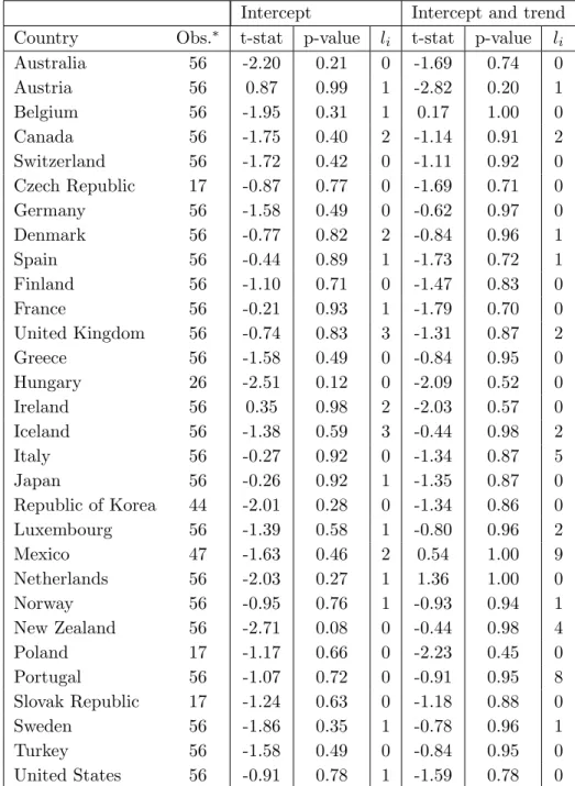
In summarising table 1, the following can be observed: On the 10% level of significance for the ADF regressions including only an intercept, the null hypothesis of non-stationarity is rejected only for New Zealand. When concentrating on the outcomes of the ADF tests which employ an intercept and trend specification, the null hypothesis is not rejected for any of the countries in the cross section. Overall, regarding hours worked as non-stationary time series is favoured over a trend stationary specification.
However, ADF tests lack power relative to the alternative that the series is a persistent, but stationary process. For example, this lack of discriminatory power is one of the reasons why Christiano, Eichenbaum and Vigfusson (2003) regard classical univariate unit root diagnostics not helpful in deciding whether to treat hours worked for the US as trend or difference stationary stochastic process.5 Increasing power of unit root tests through the
pooling of information across countries is the primary aim of panel unit root tests and a reason for the popularity of these tests. Therefore, testing the order of integration of hours worked with the help of panel data seems to offer an obvious solution to the power problem. The next section gives a brief outline of the panel assumptions and hypothesis employed in the remainder of the paper.
4Constant behaviour of hours worked per worker is a feature of the balanced growth path if the number
of workers grows with population in the long-run.
5Christiano, Eichenbaum and Vigfusson (2003) circumvent deciding on the basis of univariate unit
toot tests. Instead, they employ an encompassing criterion to select between the competing specifications. Cf. pp.8 for details.
Table 1: IndividualADF(li) test statistics
Intercept Intercept and trend Country Obs.∗ t-stat p-value l
i t-stat p-value li Australia 56 -2.20 0.21 0 -1.69 0.74 0 Austria 56 0.87 0.99 1 -2.82 0.20 1 Belgium 56 -1.95 0.31 1 0.17 1.00 0 Canada 56 -1.75 0.40 2 -1.14 0.91 2 Switzerland 56 -1.72 0.42 0 -1.11 0.92 0 Czech Republic 17 -0.87 0.77 0 -1.69 0.71 0 Germany 56 -1.58 0.49 0 -0.62 0.97 0 Denmark 56 -0.77 0.82 2 -0.84 0.96 1 Spain 56 -0.44 0.89 1 -1.73 0.72 1 Finland 56 -1.10 0.71 0 -1.47 0.83 0 France 56 -0.21 0.93 1 -1.79 0.70 0 United Kingdom 56 -0.74 0.83 3 -1.31 0.87 2 Greece 56 -1.58 0.49 0 -0.84 0.95 0 Hungary 26 -2.51 0.12 0 -2.09 0.52 0 Ireland 56 0.35 0.98 2 -2.03 0.57 0 Iceland 56 -1.38 0.59 3 -0.44 0.98 2 Italy 56 -0.27 0.92 0 -1.34 0.87 5 Japan 56 -0.26 0.92 1 -1.35 0.87 0 Republic of Korea 44 -2.01 0.28 0 -1.34 0.86 0 Luxembourg 56 -1.39 0.58 1 -0.80 0.96 2 Mexico 47 -1.63 0.46 2 0.54 1.00 9 Netherlands 56 -2.03 0.27 1 1.36 1.00 0 Norway 56 -0.95 0.76 1 -0.93 0.94 1 New Zealand 56 -2.71 0.08 0 -0.44 0.98 4 Poland 17 -1.17 0.66 0 -2.23 0.45 0 Portugal 56 -1.07 0.72 0 -0.91 0.95 8 Slovak Republic 17 -1.24 0.63 0 -1.18 0.88 0 Sweden 56 -1.86 0.35 1 -0.78 0.96 1 Turkey 56 -1.58 0.49 0 -0.84 0.95 0 United States 56 -0.91 0.78 1 -1.59 0.78 0
Notes: ∗total number of Observations. All tests were executed with the help ofEviews 5.1. MacKinnon
(1996) p-values. Lag lengthliwas chosen due to the minimum of the modified Schwarz information crite-rion. Maximum lag length was 3, 5, 9 or 10, depending on individual number of time series observations from the intervall [17,56].
4
Panel analysis
4.1
The panel unit root framework
Surveys of panel unit root tests are given by, among others, Breitung and Pesaran (2005), Choi (2004), Banerjee (1999) and with a special focus on second generation panel unit root tests by Gutierrez (2005), Jang and Shin (2005) and Gengenbach, Palm and Urbain (2004). Only the basic framework is given below.
It is assumed that the time series for N cross sections evolve according to:
hit=dit+xit (1)
xit =φixit−1+uit (2)
where i = 1, ..., N, t = 1, ..., Ti and dit represents deterministic components including
any individual intercepts or individual time trends or both. The cross section specific autoregressive coefficient isφi. Equations (1) and (2) translate into an expression for the
observable variables:
hit=φihit−1 +dit−φidit−1+uit (3)
Panel unit root tests of the first generation assume independent units hit and typically
suppose that the idiosyncratic disturbances uit are i.i.d. across i and t with E(uit) = 0,
E(u2
it) =σ2i and E(uit4)<∞.6 Examples of the modelling strategy ofuit in the presence
of cross section dependence are given below.
Most panel unit root tests build their testing strategy around ADF type regressions cor-responding to equation (3).
A test for the presence of a unit root in the panel is represented by the null hypothesis
H0 :φ1 = · · ·=φN =φ = 1. Two types of tests can be distinguished, dependent on the
alternative hypothesis under consideration. The first type of test considers a homogeneous alternative, i.e. it takes the form H1 :φ1 =· · ·=φN =φ <1. Examples are the tests of
Levin, Lin and Chu (2002), Breitung (2000) and Hadri (2000). The second sort of tests employs a heterogeneous alternative hypothesis: H1 : ∃i with φi < 1, i = 1, ..., N. This
implies that there is a subgroup N0 ≤ N for which φ1 <1, ..., φN0 <1. The tests of Im, Pesaran and Shin (2003), Maddala and Wu (1999) or Choi (2001) involve this alternative hypothesis.7 Irrespective of the alternative under consideration, when the null hypothesis
of a unit root is rejected, one can only conclude that a certain fraction of units in the
6Cf. for example, Breitung and Pesaran (2005), pp.4
7Breitung and Pesaran (2005) note, that despite the different treatment of the alternative hypothesis,
panel is stationary. The panel unit root tests under cross section dependence outlined in the subsequent sections assume a heterogeneous alternative throughout.
As mentioned above, the advantage for testing the unit root hypothesis on the basis of cross sectional time series is the amplification of power. The gain in power by switching from univariate unit root tests to panel unit root tests is well documented for example in the papers of Levin and Lin (1992) and Levin, Lin and Chu (2002).
However, if the panel features cross section dependence, classical panel unit root tests suffer from serious size distortions. As it is shown in the next section, the panel data of hours worked for OECD countries is characterised by significant cross section correlation that should not be neglected in unit root testing. Therefore, outcomes of first generation panel tests for unit roots in hours worked are not reported here.
The implication of cross section dependence is surveyed by several authors. Gengen-bach, Palm and Urbain (2004) give a brief literature overview to simulation studies that assess the performance of panel unit root tests under the presence of cross correlation and cross section cointegration. Banerjee et al. (2005) demonstrate how panel unit root tests become oversized in the presence of long-run cross unit relationships. Hassler and Tarcolea (2005) also conclude by investigating nominal long-term interest rates for 12 OECD countries that ignoring or modelling cross-correlation in multi-country stud-ies may heavily affect the outcome of non-stationarity panel analyses. Pesaran (2005) demonstrates by means of Monte Carlo simulations that panel unit root tests that do not account for cross section dependence can be seriously biased if the degree of dependence is sufficiently large. Phillips and Sul (2003) show that OLS estimators provide little gain in precision compared with single equation OLS when cross section dependence is ignored in the panel regression. Furthermore, commonly used panel unit root tests are no longer asymptotically similar under the presence of cross section dependence. Strauss and Yigit (2003) demonstrate that the greater the extent of cross correlations and their variation, the higher is the size distortion of the Im, Pesaran and Shin (2003) test.
4.2
Cross section dependence in the panel of hours worked
There are several potential causes for cross section dependence in the present panel: Common observed and unobserved factors or general residual correlation that remains after controlling for common influences. Examples for such factors affecting average hours worked are the above-mentioned technology shocks.Pesaran (2004) proposes a simple test for error cross section dependence that has correct size and sufficient power even in small samples. To check if the OECD panel at hand is characterised by cross section dependence, the residuals of the individual ADF(li)
regressions from the preceding single country analysis are used to compute Pesaran’s (2004) test statistic. The test draws on the residuals of both the intercept only and the
intercept and linear trend specifications. The test statistic of cross section dependence for an unbalanced panel is computed as8
CD = s 2 N(N −1) NX−1 i=1 N X j=i+1 p Tijρˆij ! , (4)
where ˆρij are the pairwise correlation coefficients from the residuals of the ADF
regres-sions. The correlations are computed over the common set of observations Tij for i and
j, i 6= j. The CD statistic is distributed standard normal for Tij > 3, if the number of
country specific observations exceeds the number of regressors in the underlying equation and sufficiently large N. As Pesaran(2004) demonstrates the good performance of the CD test in small samples, it seems to be well suited for the present cross section of 30 countries with numbers of time observations ranging from 17 to 56.
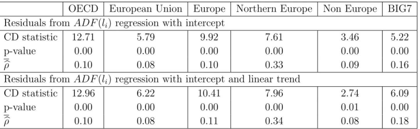
Table 2: Test of cross section dependence within different regions
OECD European Union Europe Northern Europe Non Europe BIG7 Residuals fromADF(li) regression with intercept
CD statistic 12.71 5.79 9.92 7.61 3.46 5.22
p-value 0.00 0.00 0.00 0.00 0.00 0.00
b
ρ 0.10 0.08 0.10 0.33 0.09 0.16
Residuals fromADF(li) regression with intercept and linear trend
CD statistic 12.96 6.22 10.41 7.96 2.74 6.09
p-value 0.00 0.00 0.00 0.00 0.01 0.00
b
ρ 0.10 0.08 0.11 0.34 0.08 0.18
Notes: CD test is based on the residuals of the individual ADF(li) regressions, sample is unbalanced, i.e. Ti ∈[17,56]. The CD statistic is asymptotically normally distributed. P-values refer to a two-sided test. ρbis the simple average of the pair-wise residual correlation coefficients.
OECD=Australia, Austria, Belgium, Canada, Switzerland, Czech Republic, Germany, Denmark, Spain, Finland, France, United Kingdom, Greece, Hungary, Ireland, Iceland, Italy, Japan, Republic of Korea, Luxembourg, Mexico, Netherlands, Norway, New Zealand, Poland, Portugal, Slovak Republic, Sweden, Turkey, Unites States
European Union=Austria, Belgium, Czech Republic, Germany, Denmark, Spain, France, United Kingdom, Greece, Hungary, Ireland, Italy, Luxembourg, Netherlands, Poland, Portugal, Slovak Republic, Sweden
Europe=Austria, Belgium, Switzerland, Czech Republic, Germany, Denmark, Spain, Finland, France, United Kingdom, Greece, Hungary, Ireland, Iceland, Italy, Luxembourg, Netherlands, Norway, Poland, Portugal, Slovak Republic, Sweden
Northern Europe=Denmark, Finland, Iceland, Norway, Sweden
Non Europe=Australia, Canada, Japan, Republic of Korea, Mexico, New Zealand, Turkey, USA
BIG7=Canada, Germany, France, United Kingdom, Italy, Japan, USA
Table 3: Cross section dependence across Europe and Non European countries ADF with intercept ADF with intercept and trend
CD statistic 4.60 4.67
p-value 0.00 0.00
b
ρ 0.03 0.04
Notes: CD test is based on pair-wise resdidual correlations between each european and non european country. See table 2 for further notes.
Table 2 shows the CD statistics for countries within the OECD, the European Union, Northern Europe, Non-European countries and the Big Seven western industrial coun-tries. The upper part of table 2 contains CD statistics that employ residuals from ADF estimations with intercept only while the lower part displays the results that rely on ADF residuals from a intercept and linear trend regression. The hypothesis of zero cross section correlation is rejected for all regions and both ADF specifications at the 1%-level of signifi-cance. In both specifications, according to the average correlation coefficients, the highest degree of cross section dependence is found for the countries within the group of Northern Europe, followed by the countries within the Big 7. The group of Non-European countries shows about the same degree of dependence as the countries within the European Union and within geographical Europe.
The CD statistic can also be used to test for dependence across regions with distinct countries. Table 3 displays the CD statistic that builds on correlations which are computed for the ADF residuals of each European country with the residuals of each Non-European country.9 By rejecting the null hypothesis of cross section indepencence at the 1%-level,
these test statistics also indicate the presence of error dependence across the countries of Europe and the group of Non-European countries. However, the average residual correlation coefficient ρbis rather low.
Overall, the outcomes of the preceding tests clearly indicate the presence of cross section dependence of hours worked in the panel of OECD countries. In addition, the estimates of the average correlation coefficients for different regions suggests that residual correlation is rather heterogeneous than homogeneous.
Tests for the presence of unit roots in hours worked should take these dependence into account in order to produce reliable results. The next section addresses this issue by applying second generation unit root tests for panel data.
9For this version of the test, the CD statistic is calculated as CD
N1N2 = q 1 N1N2 PN1 i=1 PN1+N2 j=N1+1 p Tijρˆij
, whereas N1 is the number of countries in region 1 and N2 is
4.3
Panel unit root tests for cross sectionally dependent panels
In this section, five different panel unit root tests which allow for cross section dependence among units are illustrated and the respective procedures are applied to the OECD sample of hours worked. These tests originate from Demetrescu, Hassler and Tarcolea (2005, DHT hereafter), Pesaran (2005, Pesaran hereafter), Phillips and Sul (2003, PS hereafter), Moon and Perron (2004, MP hereafter) and Bai and Ng (2004, BN hereafter).10 Pesaran, PS,MP and BN assume cross section dependence arising from common unobserved factors, while the DHT test builds on a modified inverse normal method to account for dependency in the data. The advantage of the test procedures of DHT and Pesaran is that they can be applied to unbalanced panels, while the tests of PS, MP and BN require balanced panels. In that case, balancing the panel reduces the cross section dimension to N = 24 and fixes the time dimension to T = 56.11
The testing strategy builds on the briefly sketched approach in Gengenbach, Palm and Urbain (2004): In a first step, the tests of DHT, Pesaran, PS and MP are used to test for the presence of a unit root in the data. If cross section dependence is due to common factors and unit roots were indicated in the first step, the BN procedure is employed to test for the presence of unit roots in the idiosyncratic components and the common factors separately. In addition, this amounts to a test for no cointegration among the individual time series of hours worked.
4.3.1 Demetrescu, Hassler and Tarcolea (2005, DHT)
The DHT test directly builds on the test statistics of the outcomes of the individual ADF tests from section 3. The test statistic is constructed as a linear combination of individual specific probits ti corresponding to the p-values pi resulting from the individual unit root
tests. The probits are quantiles from the standard normal distribution of the respective p-values. This proceeding corresponds to the inverse normal method and DHT propose a modified version for panel unit root testing to account for dependencies in the probits. These dependencies in turn stem from the dependencies in the underlying test statistics and reflect cross section dependence.
The recommended (unweighted) test statistic by DHT due to Hartung (1999) to test for a unit roots in the panel against the heterogeneous alternative is 12
10Tests that build on a GLS approach are not considered in the present analysis as they rely on T
being substantially larger thanN which is not the case for the panel data at hand. Cf. e.g Breitung and Das (2005).
11Balancing the panel drops the observations for the Czech Republic, Hungary, Mexico, Poland, Slovak
Republic and the Republic of Korea.
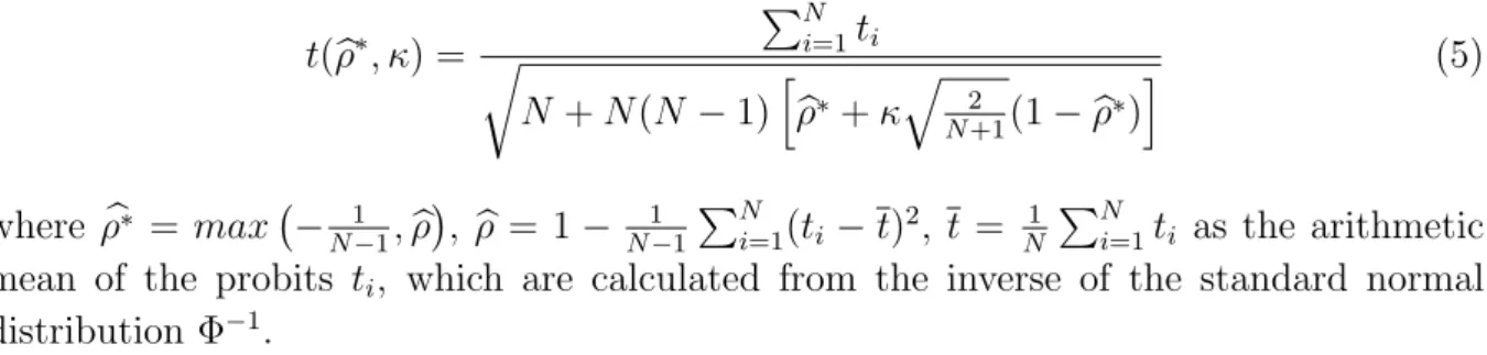
t(ρb∗, κ) = PN i=1ti r N +N(N −1)hρb∗+κ q 2 N+1(1−ρb∗) i (5) where ρb∗ = max − 1 N−1,ρb , ρb= 1− 1 N−1 PN i=1(ti −t)2, t = N1 PN i=1ti as the arithmetic
mean of the probits ti, which are calculated from the inverse of the standard normal
distribution Φ−1.
The contribution of DHT is to show that under which conditions the statistic of (5) follows a standard normal distribution. In addition, it is demonstrated that the test is robust if the correlation of the probits is varying at a certain degree. Furthermore, on experimental grounds, DHT provide evidence that the modified inverse normal method is reasonably reliable when applied to ADF tests in correlated panels. This holds also whenN = 25 and
T = 50 but it is shown that the modified inverse normal method results in an undersized test in the presence of weak correlation.
The test statistict(ρb∗, κ) is readily computed with the p-values from table 1. The value of
b
ρ∗ amounts to 0.16 in the intercept case and to 0.05 in the intercept and trend case. DHT and Hartung (1999) propose to use κ = κ1 = 0.2 or κ = κ2 = 0.1(1 + N1−1 −ρb∗). This
parameter is meant to regulate the actual significance level in small samples.13 In the
simulation studies of DHT, the experimental size of the test is not sensitive to the choice of κ.14 The test statistic here is slighty influenced by the choice ofκ in the intercept and
trend case. However, the test decision is not affected by this option. Table 4 shows test results.
Table 4: Results of modified inverse normal method
Intercept Intercept and trend
t(ρb∗, κ1) 0.72 3.63 p-value 0.76 1.00
t(ρb∗, κ2) 0.76 4.02 p-value 0.78 1.00
Notes: Test statistics are based on MacKinnon (1996) p-values of individual ADF tests. N = 30 and Ti∈[17,56].
The low level of significance for both the intercept only and intercept and trend specifi-cation clearly implies not rejecting the homogeneous unit root hypothesis.
13Cf. Hartung (1999) for details.
14However, DHT assume stronger correlation in their simulation study than it is indicated for hours
4.3.2 Pesaran (2005, Pesaran)
It is well conceivable that cross section dependence in international data on hours worked can occur because of common global factors like a global trend or cyclical element. The country figures suggest that there is co-movement between hours worked (see figures 4 to 7 in the appendix). The Pesaran test and also the subsequent methods do account for cross section dependence through the assumption that one or more common unobserved factors are driving the dependence structure.
Pesaran builds on the assumption that the error terms uit of equation (3) follow a single
common factor structure
uit=λift+it (6)
The common unobserved factor ft is always assumed to be stationary and impacts the
cross section times series with a fraction determined by the individual specific factor loading λi. For the idiosyncratic errors it, the same assumptions as under the panel
unit root tests of the first generation hold, i.e. they are are i.i.d. across i and t with
E(it) = 0, E(2it) = σi2 and E(4it) < ∞. Furthermore, it, ft and λi are mutually
independent distributed for all i.
Thus, cross section dependence arises due to the common factor, which can be approx-imated by the cross section mean ht = N1
PN
i=1hit.15 Pesaran proposes the following
augmented Dickey-Fuller regression:
∆hit=ai+αihit−1+βiht−1+ p X j=1 γij∆hit−j + p X j=0 θij∆ht−j+dit+εit (7)
The test for the presence of a unit root can now be conducted on the grounds of the t-value of αi either individually or in a combined fashion. The first satistic is denoted as
cross sectionally augmented Dickey-Fuller CADFi statistic while the latter resembles the
familiar IPS statistic of Im, Pesaran and Shin (2003) and is constructed as
CIP S = 1 N N X i=1 CADFi (8)
Pesaran investigates the performance of theCADFi and CIP S tests by means of Monte
Carlo simulations and shows that these tests have satisfactory size and power even for relatively small values of N and T, i.e. even in the case of N = T = 10. In the linear
15If a common time specific effect is the only source of cross section correlation, the correlation can be
eliminated by subtracting cross sectional means from the data. Pesaran, Shin and Smith (1995) propose this proceeding. However, Strauss and Yigit (2003) demonstrate through Monte Carlo simulation that demeaning the data leads to false inference in panel unit root tests if the original data generating process had heterogeneous correlation, i.e. if pair-wise cross-section covariances of the error components differ across units.
trend model, power rises quite rapidly with both N and T if T >30. This small sample property renders the Pesaran test quite appealing for an application to the present OECD cross section.
Due to the presence of the lagged level of the cross sectional average, the limiting distri-bution of theCADFi statitics and theCIP S statistic does not follow a standard
Dickey-Fuller distribution. However, Peseran provides critical values based on simulations for the CADF and CIPS-distributions for three cases (no intercept and no trend, intercept only, intercept and trend).
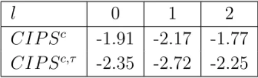
Table 5 reports the results of the CIP S test for hours worked for the unbalanced OECD panel and different lag length l.
Table 5: Results of the CIP S test
l 0 1 2
CIP Sc -1.91 -2.17 -1.77
CIP Sc,τ -2.35 -2.72 -2.25
Notes: Entries are averages of t-values. CIP Sc is based on individual CADF regressions with l lags of differences including an intercept only, while CIP Sc,τ is based on CADF regressions including an intercept and trend. Critical values forN = 30 andT = 50 are tabulated in Pesaran (2005). They are -2.30/-2.16/-2.08 for the 1%/5%/10% level of significance in the intercept only case, and -2.78/-2.65/-2.58 for the intercept and trend case. N = 30 andTi∈[17,56].
TheCIP S statistic is not smaller than any of the critical values corresponding to the 1%, 5% or 10% level of significance for all specifications. The case when l = 1 in the trend and intercept model is an exception. Here, the test indicates stationarity at the 5% level of significance. Otherwise, the outcomes are not very sensitive to the choice of number of lagged differences l. Thus, on the basis of the common unobserved factor assumption for the error process, the Pesaran test gives indication of non-stationarity of hours worked.
4.3.3 Phillips and Sul (2003, PS)
PS also assume that cross section dependence arises from a single common factor in uit.
The errors uit follow the same data generating process as in equation (6). Similar to
Pesaran, the idiosyncratic errors it are i.i.d with variance σi2, the factor loadings are
non-stochastic and the common factor ft is i.i.d. N(0,1).
The idea of PS is to remove this common factor effect by pre-multiplying the original data with a projection matrix Fbλ, thereby eliminating cross section dependence. The
projection matrix Fbλ is obtained by an orthogonalisation procedure that builds on a
Σ of the idiosyncratic errors.16 Following the terminology of Jang and Shin (2005), this
proceeding will be denoted projection de-factoring.
The transformed data h+it = Fbλhit is then used to perform individual ADF regressions.
Sinceh+it are asymptotically uncorrelated across i, standard panel unit root tests with the de-factored data are feasible.
PS propose to combine p-values of the univariate ADF regressions with de-factored data to construct meta-statistics just as in Choi (2001) or DHT to test for unit roots in the panel.17 The first test statistic is a Fisher type and given by18
P =−2
NX−1
i=1
ln(pi) (9)
while the second statistic is a inverse normal test, denoted
Z = √1 N NX−1 i=1 Φ−1(p i) (10)
Once again,pi defines the p-values of the univariate ADF tests with de-factored data and
Φ−1 is the inverse of the standard normal distribution. For fixed N and as T
→ ∞, P
converges to a χ2
2(N−1) distribution and Z to a standard normal distribution.
PS provide guidance to the small sample performance of their proposed tests via Monte Carlo experiments. It is shown that the tests have good size and power properties even in cases were N = 10 and T = 50.19 The results for the PS panel test for a homogeneous
unit root in average hours worked is reported in table 6. Note that the test results rely on a balanced panel.
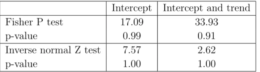
Both the P and the Z statistic strongly imply not rejecting the unit root hypothesis for the intercept only as well as the intercept and trend specification.
So far, the test of Pesaran and PS failed to reject the unit root hypothesis for hours worked when allowing a single factor structure in the composite error term. In the next
16Cf. PS, p. 237 for details to the orthogonalisation procedure.
17In fact, PS propose two additional statistics to test for a homogeneous unit root in the panel that
build directly on the coefficient estimates of the individual autoregressive parameters. PS refer to them asGtests. However, as PS demonstrate by means of simulation experiments that theP andZ test have considerably greater power than theGtests, they are not pursued here.
18The sums of the test statistics goes overi toN
−1 since the transformation due to removal of the cross section dependence in the limit reduces the panel to dimensionN−1. Cf. PS, p. 238.
19Jang and Shin (2005) report an experimental size of 9.7% at the 5% nominal level for the PS panel
unit root procedure and a sample withN = 25 and T = 50. However, their experiment is not strictly comparable to the PS experiment since Jang and Shin (2005) base statistics on simple averages of t-values instead of considering theP andZ statistics.
Table 6: Results of PS panel test
Intercept Intercept and trend Fisher P test 17.09 33.93
p-value 0.99 0.91
Inverse normal Z test 7.57 2.62
p-value 1.00 1.00
Notes: Computational work was performed in GAUSS. A GAUSS code is available from Donggyu
Sul. Here, the lag order of the univariate ADF regressions is chosen based on the top-down method. Maximum number of lags was set to 10. N = 24 andT = 56.
section, it is investigated if there is more than one factor causing the dependence pattern of the data.
4.3.4 Moon and Perron (2004, MP)
The MP test for a homogeneous unit root is similar to the PS test in that it also removes dependency that arises from common factor by projection de-factoring. Yet it differs from the PS proceeding mainly in two ways. First, it allows cross section dependence to originate from more than one common factor. Secondly, the derivation of the projection matrix differs from the PS method. MP estimate the factor loadingsλi, which are required
to obtain the projection matrix, by a principal component estimation scheme. MP assume that the error term from equation (3) follows
uit =λ0ift+eit (11)
where in this case ft is a (K ×1) vector of common unobserved factors and λi is the
corresponding (K×1) vector of factor loadings. Similar to the assumptions of Pesaran and PS, the idividual specific error componentseitand the common factorsftfollow stationary
and invertible M A(∞) processes that are independent of each other.20 In the unit root
case,φi = 1 in equation (3) and this implies that the factors and idiosyncratic components
integrate to Pts=1fs and
Pt
s=1eis, respectively. By assumptions, MP allow the
non-stationary factors to cointegrate while cointegration among the integrated idiosyncratic errors is excluded.
MP’s testing procedure is summarised as follows. In a first step, under the null hypoth-esis of a homogeneous unit root in equation (3), the pooled OLS estimator φbpool of the
autoregressive coefficient is obtained. This estimator is used to construct an estimate of the composite error terms buit = hit −φbpoolhit−1 and by means of principal components
analysis, an estimate of the factor loadings Λ = (b bλ1, ...,λbN)0 is attained. The (N ×K)
matrix Λ is then utilised to construct the projection matrixb QΛ = IN −Λ(b Λb0Λ)b −1Λb0 for
removing common factor effects from the original data. However, this procedure requires the knowledge of the number of common factorsK. In practise, this not the case and the number of factors need to be estimated. For these purposes, MP suggest to use the infor-mation criteria of Bai and Ng (2002) which necessitate the setting of a maximal number
Kmax of factors.
With the projection matrix at hand, MP propose the following modified pooled estimator of the de-factored data:21
b ρ∗ pool = tr(H−1QΛH0)−N TbγeN tr(H−1QΛH−0 1) (12) In equation (12), tr(.) is the trace operator and γbN
e an estimator of the cross-sectional
average of the one-sided long-run variance of the idiosyncratic errors eit in (11) and is
meant to account for serial correlation in the transformed idiosyncratic errors eit.
MP suggest to use the following t-statistics for testing the homogeneous unit root hy-pothesis against the heterogeneous alternative:
t∗ a= √ N T(ρb∗ pool −1) p 2ϕb4 e/bω4e (13) t∗ b = √ N T(ρb∗ pool−1) r 1 N T2tr(H−1QΛH−01) b ωe b ϕ2 e (14) Equation (13) and (14) involve estimators of the long-run variancesω2
ei ofeit, where bω
2
e is
an estimator for the cross sectional average of bω2
ei andϕb
4
e a cross sectional average ofωbe4i. As MP note, averaging the individual specific long-run variances should remove some of the uncertainty inherent in estimation of long-run variances and improve unit root testing over univariate counterparts. However, bias in the estimation of these variances will not be removed through averaging.
MP show that under the null hypothesis, the statistics t∗
a and t∗b converge to a standard
normal distribution as N → ∞and T → ∞ with N/T →0.
MP also demonstrate that their tests have no power against local alternatives in the case where heterogeneous deterministic trends exit in the data. Therefore, the tests should not be used if one assumes linear time trends in the deterministic components of the data generating process of (3).
The simulation experiments of MP confirm the good power and size results of the t-tests, especially when T = 300. They also conclude that the number of factors is estimated
21The vectors h
i = (hi2, ..., hiT) and hi,−1 = (hi1, ..., hiT−1) have been horizontally concatenated to
imprecisely for a small number of cross sections (N = 10). If the number of cross-sections is at least 20, the number of factors can be estimated with high precision.22 Since MP do
not consider samples with less than 100 time series observations in their simulation, the applicability of the MP procedure for the present panel data of hours worked is assessed with help of the experiments of Gengenbach, Palm and Urbain (2004) and Gutierrez (2005).
From the tables of Gengenbach, Palm and Urbain (2004)23 it can be seen that both
statistics of MP have rejection frequencies lower than the nominal size if T = 50 and
N = 10 or N = 50, irrespective of whether the non-stationarity originates from the idiosyncratic components or common factors. For the near unit root case, power of the MP test is good if N >10.
Although Guiterrez (2005) concludes that the MP tests in general show good size and power for various values of N and T and different model specifications, the results also indicate that forN = 20 andT = 50 the t∗
a is undersized whilet∗b has in general rejection
frequencies higher than the nominal size.24
As mentioned above, in applied work the number of common factors needs to be estimated. In conducting the MP test for hours worked, the seven information criteria for estimating the number of factors that are due to Bai and Ng (2002) are considered.25
The application of the information criteria to the logarithm hours worked in the balanced OCED panel results in inconclusive estimates of the number of factors. The criteria
P Cp1,P Cp2,P Cp3 andICp3 are highly sensitive to the choice of Kmax and always choose
the maximum number Kmax. IC
p1 selects two numbers of factors if Kmax is less than
12. For Kmax > 12, the chosen number of factors by IC
p1 also strictly monotonically
increases withK =Kmax and always ends up with K =Kmax. The criteria IC
p2 always
prefers K = 1 as long as Kmax < 17. For Kmax > 17, the chosen number of factors is
Kmax. BIC
3 also prefers one factor as long as the maximum number does not exceed 6.
For higer values of Kmax, the BIC
3 monotonically increases as well. The latter is the
preferred criteria of MP in small samples.26
Congruent results are obtained when setting Kmax = 6 and focusing on IC
p2 and BIC3
in which case it is recommended to assume one common factor. However, for robustness check, the case K = 2 andK = 6 is also considered below. Under the assumption of one common factor, the data generating processes of the MP, PS and Pesaran tests are the
22This is due to Bai and Ng (2002).
23Cf. Gengenbach, Palm and Urbain (2004), pp. 26. The comments refer to the simulation results
assuming a single common factor
24CF. Guiterrez (2005), p. 11, table 1.
25Cf. MP, pp. 93 or Bai and Ng (2002), pp 201 for a detailed description of these information criteria. 26In absence of a formal criterion, MP and Bai and Ng (2002) setKmax= 8 in their simulation studies for all values ofN andT.
same and the only difference is in the treatment of the common unobserved factor in the estimation strategy.
As in MP, the long-run variances are estimated using the Andrews and Monahan (1992) method. Tabel 7 shows results of the MP panel unit root test for hours worked.
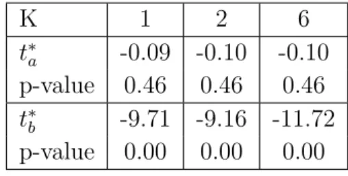
Table 7: Results of MP panel test
K 1 2 6 t∗ a -0.09 -0.10 -0.10 p-value 0.46 0.46 0.46 t∗ b -9.71 -9.16 -11.72 p-value 0.00 0.00 0.00
Notes: Computational work was performed in Matlab. A Matlab code is available from Benoit Perron.
Intercept only case. N = 24 andT = 56.
The t∗
a statistic implies not rejecting the null of a homogenous unit root in the panel for
the assumption of one, two or six common factors. In contrast, thet∗
b statistics rejects for
all specifications. When considering the results of both test statistics, the conclusions to be drawn are highly contradictory. There is some evidence that thet∗
b statistic is oversized
in small samples in Gutierrez (2005). Since there is no general guidance as to which t-statistic should be preferred in applied settings, the MP test alone offers no direction in the present analysis. However, the results of the previous tests suggest to put more confidence into the t∗
a in the present estimation and to conclude that the MP panel unit
root test also fails to reject the null hypothesis.
4.3.5 Bai and Ng (2004, BN)
Instead of treating the common factors as a nuisance, they become a direct object of further investigation in the BN testing framework. BN build on very similar assumptions as MP. BN call their testing procedure Panel Analysis of Non-stationarity in Idiosyncratic and Common components (PANIC), whereas the acronym nicely summarises the intended aim: While allowing the data being driven by one or more common factors and idiosyn-cratic components, the time series properties of these elements are assessed separately without a priori knowledge whether these elements are stationary or integrated. Since the panel unit root tests give evidence for the non-stationarity of hours worked so far, the BN test is employed to determine the source of non-stationarity. On the grounds of the previous analysis, it is assumed throughout that hours worked are driven by idiosyncratic elements and a single unobserved common factor.27
27If there is more than one common integrated factor, these factors need to be tested for cointegration
In the presence of a single common factor, the data generating process of BN is
hit =dit+λiFt+Eit (15)
where the common factor Ft and the idiosyncratic errors Eit follow AR(1) models with
a polynomial lag structure of i.i.d. shocks. Concerning the deterministic elements dit,
an intercept or a trend or both are allowed. If the errors Eit are independent across
units, i.e. if the cross section dependence can be effectively represented by a common factor structure like in the Pesaran, PS and MP setting, pooled tests for unit roots in the idiosyncratic components are feasible. An appealing feature of the pooled tests is that they can be regarded as a panel test of no cross-member cointegration. The workings of the latter will be demonstrated below.
The strategy to consistently estimate the individual components of (15) even if some or all elements of Ft and Eit are integrated of order one is as follows. In a first step, the
hit’s are differenced if the deterministics include only an intercept or are differenced and
demeaned if dit includes and intercept and trend.28 Like in MP, the principal component
method is employed with the differenced data and the common factors, factor loadings and residuals are estimated.
In a next step, the estimates of the differenced factors and idiosyncratic error components are re-integrated `a la xbt =
Pt
s=2∆xbs and separately tested for unit roots. Let Ebit and
b
Ft be the re-integrated estimates of the common factor and idiosyncratic components.
Since Ebit = hit −bλiFbt, Jang and Shin (2005) denote such a proceeding as subtraction
de-factoring. For unit root testing, BN propose to employ the usual t-statistics of ADF regressions in the common factor and idiosyncratic components, respectively. For the model with an intercept only, the t-statistics to test the common factor for a unit root is denoted ADFc
F. If the model contains an intercept and linear trend, the statistic is
ADFFc,τ. Accordingly, the t-statistics for individual unit root tests of the idiosyncratic components are denoted ADFc
E(i) and ADF c,τ E (i).
BN show that the asymptotic distribution of ADFc
E(i) coincides with the usual DF
dis-tribution (no intercept), while ADFc
F has the same limiting distribution as the DF test
for the intercept only case. Furthermore, ADFFc,τ follows a DF distribution for the case with intercept and trend in the limit. However, the limiting distribution of ADFEc,τ(i) is proportional to the reciprocal of a Brownian bridge and critical values are not tabulated yet and need to be simulated.29
For independent Eit, BN propose a pooled test for unit roots in Ebit due to Choi (2001)
that builds on combining p-values pc
E(i) of ADF c
E(i) and are similar to the test statistics
of PS and DHT: Pc E = −2PNi=1lnpc E(i)−2N √ 4N (16)
28For details to this procedure, cf. BN, pp. 1137
The test statistic Pc
E is asymptotically distributed standard normal. The hypothesis of
a homogeneous unit root in the idiosyncratic components is rejected for large positive values Pc
E.
The pooled test can also be regarded as a panel test of no cross-member cointegration since no stationary combination of the individual variableshit can be obtained such that
the unit root hypothesis holds for all i. On the other hand, if the common factor is integrated of order one and there are some stationary Eit’s, then the common factor and
the stationary variables are cointegrated with vector (1,−λi)0. If the PEc statistic rejects
and all idiosyncratic components can be seen as stationary, the hit’s cointegrate and the
matrix QΛ of MP for de-factoring the data serves as a cointegration matrix. 30
BN enrich their work with simulation studies to investigate the small sample performance of the PANIC procedure. They conclude that the proposed tests have good power even when N = 40 and T = 100. However, these values are nearly twice as large as the panel dimension of hours worked. Jang and Shin (2005) find that tests based on the BN method have sizes close to the nominal level when T = 50 and N = 25 and power is slightly better than for the PS and MP procedure. In the case where a unit root is present in the common factor and in all idiosyncratic errors, the simulation experiment of Gegenbach, Palm and Urbain (2004) show that the tests of BN for the intercept only case have rejection frequencies close to the nominal size even when N = 10 and T = 50. If there is a unit root in the common factor and the idiosyncratic components are near unit root, the ADFc
F rejects with a frequency at the nominal level, while P c
E has more
power thanADFc
E(i). Although the PANIC method is derived for applications with large
dimensional panels where a high number of cross sections permits consistent estimation of the common factors while the large T dimension allows application of central limit theorems, there is some simulation evidence that the BN test gives reasonable guidance also in samples of moderate size.
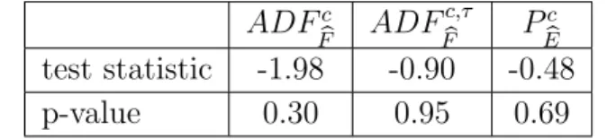
Table 8: BN results for common factor and pooled idiosyncratic components
ADFc F ADF c,τ F P c E test statistic -1.98 -0.90 -0.48 p-value 0.30 0.95 0.69
Notes: MacKinnon (1996) p-values. N = 24 andT = 56.
Results for the ADFc
F,ADF c,τ
F andP c
E test are shown in table (8). Test statistics for the
common factor are computed for the intercept and intercept and trend case. In both cases, the test does not reject and an integrated common factor can be assumed. In addition, the pooled test of the idiosyncratic errors also fails to reject in the intercept only case
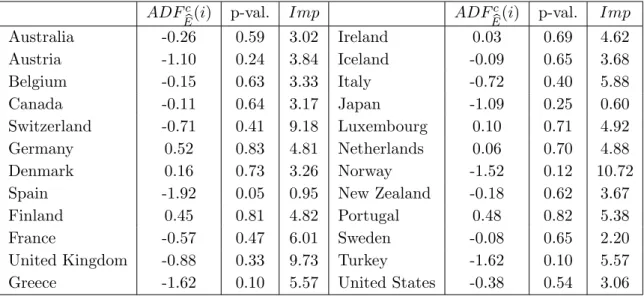
Table 9: Results of BN’s test for unit roots in idiosyncratic errors
ADFc
E(i) p-val. Imp ADF c E(i) p-val. Imp Australia -0.26 0.59 3.02 Ireland 0.03 0.69 4.62 Austria -1.10 0.24 3.84 Iceland -0.09 0.65 3.68 Belgium -0.15 0.63 3.33 Italy -0.72 0.40 5.88 Canada -0.11 0.64 3.17 Japan -1.09 0.25 0.60 Switzerland -0.71 0.41 9.18 Luxembourg 0.10 0.71 4.92 Germany 0.52 0.83 4.81 Netherlands 0.06 0.70 4.88 Denmark 0.16 0.73 3.26 Norway -1.52 0.12 10.72 Spain -1.92 0.05 0.95 New Zealand -0.18 0.62 3.67 Finland 0.45 0.81 4.82 Portugal 0.48 0.82 5.38 France -0.57 0.47 6.01 Sweden -0.08 0.65 2.20 United Kingdom -0.88 0.33 9.73 Turkey -1.62 0.10 5.57 Greece -1.62 0.10 5.57 United States -0.38 0.54 3.06
Notes: Computational work was performed inMatlab. AMatlabcode is available from Serena Ng.
MacK-innon (1996) p-values. Lag length was chosen due to the minimum of the modified Akaike information criterion. Imp= St.Dev(
λi Ft) St.Dev( Eit). N = 24 andT = 56.
so that two conclusions can be drawn. First, the non-stationarity of hours worked for which nearly all panel tests of the previous sections found evidence, seems to originate from a common as well as country specific sources. Second, the insignificance of the Pc
E
statistic implies that the non-stationarity hypothesis can not be rejected jointly. Since testing the idiosyncratic errors jointly for a homogenous unit root amounts to a test of no cointegration, the outcomes here give evidence that there is no cointegration among the individual time series of hours worked.
The results for individual unit root tests of the country specific errors are reported in table 9. The insignificance of the ADFc
E(i) for all countries except Spain confirms the
result of the Pc
E test. For Spain it can be conjectured at the 10% level of significance
that hours worked and the common factor cointegrate since these two components form a stationary linear combination.
Columns 4 and 8 of table 9 show the impact of the common factor in relation to the idiosyncratic component. This measure is calculated as the standard deviation of the country specific factor effect (bλiFbt) divided by the standard deviation of the estimated
errorsEbit. This ratio is greater than one for all countries except for Spain and Japan and
indicates that most of the variation in the logarithm hours worked arises from the common factor. For Spain and Japan, idiosyncratic elements are more important in driving the evolution of hours worked.
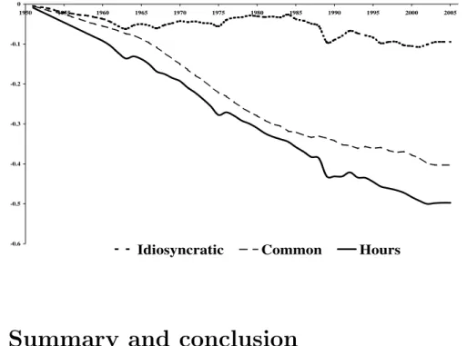
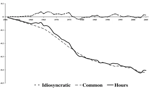
To get a visual impression of the decomposition of the BN procedure, the graphs of the estimated factor component bλiFbt and country specific elements for Japan, Germany and
Norway are depicted by the figures 1 to 3. These countries are chosen because they show a low, medium and high impact of the common factor in relation to their country specific effects. Figure 1: Japan -0.15 -0.1 -0.05 0 0.05 0.1 1950 1955 1960 1965 1970 1975 1980 1985 1990 1995 2000 2005
Idiosyncratic Common Hours
For Japan, it can be seen that the time path of hours worked is dominated by country spe-cific influences, while the German evolution of hours worked is marked by the downward trend of the common factor, which is overlaid by the idiosyncratic component. Norway, on the other side, shows a development of hours that is mainly in line with the common factor and exhibits country specific influences with a cyclical movement around the factor trend.
It is important to notice that actual hours worked and the common factor do not de-scribe some kind of equilibrium as the idiosyncratic errors, defined as the residual from the linear relationship between the country specific factor influence and actual hours, are
non-stationary. The decomposition rather shows that, although a common integrated factor can substantially influence the development of hours (e.g. Norway), the persis-tent behaviour of this variable is not solely due to a common stochastic trend but also characterised by persistent country specific determinants.
Figure 2: Germany -0.6 -0.5 -0.4 -0.3 -0.2 -0.1 0 1950 1955 1960 1965 1970 1975 1980 1985 1990 1995 2000 2005
Idiosyncratic Common Hours
5
Summary and conclusion
The results of the present analysis show that evidence in favour of the non-stationarity hypothesis of hours worked per employee in the OECD countries is vast.
Simple ADF tests for individual countries are not able to reject the unit root hypothesis both in the intercept and intercept and linear trend model.31. However, univariate unit
root tests lack power against local alternatives in finite samples. This is one of the reasons why researchers sometimes doubt the implications of these tests when the alternative under consideration is a stationary but persistent series. Panel unit root tests are able to substantially increase power over univariate tests if the panel data is cross sectionally independent. In the presence of cross section dependence, this needs to be accounted for in order to retain the high power properties of these tests.
In the present analysis, it was first shown that the cross sectional observations for hours worked are characterised by heterogeneous cross section dependence. Second, panel unit root tests of the second generation that account for this dependence were applied. For robustness reasons, five different panel unit root tests were conducted and only under rare circumstances, rejections of the homogeneous unit root hypothesis were observed.
Besides diagnosing the property of non-stationarity quite robustly, more interesting fea-tures of the data show up. When allowing hours worked to be influenced by a common
31New Zealand is the solitary exception, where the individual ADF test rejects at the 10% level of
Figure 3: Norway -0.5 -0.4 -0.3 -0.2 -0.1 0 0.1 1950 1955 1960 1965 1970 1975 1980 1985 1990 1995 2000 2005
Idiosyncratic Common Hours
factor and applying the PANIC procedure of Bai and NG (2004) to decompose the factor structure, the following stands out: Non-stationarity of hours worked originates both from an integrated common factor and an integrated idiosyncratic component. Since this holds for all countries, it is an implication for the individual time series being not cointegrated along the cross sectional dimension.
However, the empirical analysis here refers to rather abstract and intangible concepts like ‘common unobserved factors’ and ‘persistent idiosyncratic components’ which help to empirically model the data properties quite well, but give no further insights into economic relations. The cited literature in the introduction to this paper illustrates rudimentary that various candidates for persistently influencing the aggregate labour supply and for explaining cross country differences have been proposed and also empirically investigated. Further work in this direction should follow.
Based on the results of the present analysis, it is strongly recommended to transform hours worked to obtain a stationary time series if one employs econometric methods that rely on standard asymptotic theory or to use the analytical tools that have been developed for investigating non-stationary variables if one considers the level of hours worked.
References
Alesina, A., E. Glaeser and B. Sacerdote (2005): “Work and Leisure in the U.S. and Europe: Why So different?,” NBER Working Paper, 11278.
Andrews, D.W.K. and J.C. Monahan(1992): “An improved heteroskedasticity and autocorrelation consistent covariance matrix estimator,”Econometrica, 60(4), 953–966.
Bai, J. and S. Ng (2002): “Determining the number of factors in approximate factor models,”Econometrica, 70, 191–221.
(2004): “A PANIC Attack on Unit Roots and Cointegration,” Econometrica, 72, 1127–1177.
Banerjee, A. (1999): “Panel Data Unit Roots and Cointegration: An Overview,” Ox-ford Bulletin of Economics and Statistics, 61, 607–629.
Banerjee, A., M. Marcellino and C. Osbat(2005): “Testing for PPP: Should we use Panel Methods?,” Empirical Economics, 30(1), 77–91.
Blanchard, O. (2004): “The Economic Future of Europe,” NBER Working Paper, 10310.
Breitung, J. (2000): “The Local Power of Some Unit Root Tests for Panel Data,” in
Nonstationary Panels, Panel Cointegration, and Dynamic Panels, Advances in Econo-metrics, Vol. 15, ed. by B. Baltagi. JAI, Amsterdam.
Breitung, J. and M.H. Pesaran (2005): “Unit Roots and Cointegration in Panels,”
Deutsche Bundesbank Discussion Paper Series 1: Economic Studies, (42/2005).
Breitung, J. and S. Das (2005): “Panel Unit Root Tests Under Cross Sectional Dependence,” forthcoming in: Statistica Neerlandica.
Choi, I. (2001): “Unit Root Tests for Panel Data,”Journal of International Money and Finance, 20, 249–272.
(2004): “Nonstationary Panels,” forthcoming in: Palgrave Handbooks of Econo-metrics: Theoretical Econometrcis, Vol. 1.
Christiano, L., M. Eichenbaum and R. Vigfusson (2003): “What Happens After a Technology Shock?,”Federal Reserve Board, International Finance Discussion, (768).
Demetrescu, M., U. Hassler and A.-I. Tarcolea (2005): “Combining Signifi-cance of Correlated Statistics with Application to Panel Data,” forthcoming in Oxford Bulletin of Economics and Statistics.
Gal´ı, J. (1999): “Technology, Employment, and the Business Cycle: Do Technology Shocks Explain Aggregate Fluctuations?,” American Economic Review, 89(1), 249– 271.
Gengenbach, C. F. Palm and J.-P. Urbain (2004): “Panel Unit Root Tests in the Presence of Cross-Sectional Dependencies: Comparison and Implications for Mod-elling,” Research Memoranda 040, Maastricht Research School of Economics of Tech-nology and Organization.
Gutierrez, L.(2005): “Panel Unit Roots Tests for Cross-Sectionally Correlated Panels: A Monte Carlo Comparison,” forthcoming Oxford Bulletin of Economics and Statistics.
Hadri, K. (2000): “Testing for stationarity in heterogeneous panel data,”Econometrics Journal, 3, 148–161.
Hamilton, J.(1994): Time Series Analysis. Princeton University Press, Princeton, New Jersey.
Hartung, J. (1999): “A Note on Combining Dependent Tests of Significance,” Biomet-rical Journal, 41, 849–855.
Hassler, U. and A.-I. Tarcolea (2005): “Combining Multi-country Evidence on Unit Roots: The Case of Long-term Interest Rates,” Version May 13.
Im, K., M.H. Pesaran and Y. Shin(1995): “Testing for Unit Roots in Heterogeneous Panels,” DAE Working Papers Amalgamated Series No. 9526, University of Cambridge.
Im, K.S., M.H. Pesaran and Y. Shin (2003): “Testing for Unit Roots in Heteroge-neous Panels,” Journal of Econometrics, 115, 53–74.
Jang, M. J. and D.W. Shin (2005): “Comparison of panel unit root tests under cross sectional dependence,” Economics Letters, 89, 12–17.
Levin, A. and C.-F. Lin (1992): “Unit root tests in panel data: Asymptotic and finite-sample properties,”U.C. San Diego Discussion Paper 92-23.
Levin, A., C.-F. Lin and C.-S. J. Chu (2002): “Unit Root Tests in Panel Data: Asymptotic and Finite-Sample Properties,” Journal of Econometrics, 108(1), 1–24.
MacKinnon, J. (1996): “Numerical Distribution Functions for Unit Root and Cointe-gration Tests,”Journal of Applied Econometrics, 11, 601–618.
Maddala, G.S. and S. Wu (1999): “A Comparative Study of Unit Root Tests with Panel Data and A New Simple Test,” Oxford Bulletin of Economics and Statistics, 61, 631–652.
Moon, H.R. and B. Perron (2004): “Testing for a unit root in panels with dynamic factors,”Journal of Econometrics, 122, 81–126.
Nickell, S. J., and L. Nunciata (2001): “Labour Market Institutions Database,”
Centre for Economic Performance, London School of Economics, London.
Pesaran, M. (2004): “General Diagnostic Tests for Cross Section Dependence in Pan-els,” Working Paper, University of Cambridge, June.
(2005): “A Simple Panel Unit Root Test in the Presence of Cross Section Dependence,”Working Paper, University of Cambridge, January.
Phillips, P.C.B. and D. Sul (2003): “Dynamic panel estimation and homogneity testing under cross section dependence,”Econometrics Journal, 6, 217–259.
Prescott, E. (2004): “Why Do Americans Work So Much More Than Europeans,”
Federal Reserve Bank of Minneapolis Quarterly Review, 28(1), 2–13.
Strauss, J. and T. Yigit (2003): “Shortfall of panel unit root testing,” Economics Letters, 81, 309–313.
The Conference Board and Groningen Growth and Development Centre
(2006): “Total Economy Database,” January.
Wolters, J. and U. Hassler (2006): “Unit Root Testing,” Allgemeines Statistisches Archiv, 90.
Figure 4: Hours worked per worker Australia 1, 6 5 0 1, 8 0 0 1, 9 5 0 2 , 10 0 19 6 0 19 7 0 19 8 0 19 9 0 2 0 0 0 Austria 1, 4 0 0 1, 6 0 0 1, 8 0 0 2 , 0 0 0 2 , 2 0 0 19 6 0 19 7 0 19 8 0 19 9 0 2 0 0 0 Belgium 1, 4 0 0 1, 8 0 0 2 , 2 0 0 2 , 6 0 0 19 6 0 19 7 0 19 8 0 19 9 0 2 0 0 0 Canada 1, 6 0 0 1, 8 0 0 2 , 0 0 0 2 , 2 0 0 19 6 0 19 7 0 19 8 0 19 9 0 2 0 0 0 Switzerland 1, 4 0 0 1, 6 0 0 1, 8 0 0 2 , 0 0 0 2 , 2 0 0 19 6 0 19 7 0 19 8 0 19 9 0 2 0 0 0 Czech Republic 1, 8 0 0 1, 9 0 0 2 , 0 0 0 2 , 10 0 19 8 5 19 9 0 19 9 5 2 0 0 0 2 0 0 5 Germany 1, 3 0 0 1, 6 0 0 1, 9 0 0 2 , 2 0 0 2 , 5 0 0 19 5 0 19 6 0 19 7 0 19 8 0 19 9 0 2 0 0 0 Denmark 1, 3 0 0 1, 6 0 0 1, 9 0 0 2 , 2 0 0 19 5 0 19 6 0 19 7 0 19 8 0 19 9 0 2 0 0 0
Figure 5: Hours worked per worker Spain 1, 7 0 0 1, 9 0 0 2 , 10 0 2 , 3 0 0 19 5 0 19 6 0 19 7 0 19 8 0 19 9 0 2 0 0 0 Finland 1, 5 0 0 1, 7 0 0 1, 9 0 0 2 , 10 0 19 5 0 19 6 0 19 7 0 19 8 0 19 9 0 2 0 0 0 France 1, 3 0 0 1, 6 0 0 1, 9 0 0 2 , 2 0 0 19 5 0 19 6 0 19 7 0 19 8 0 19 9 0 2 0 0 0 United Kingdom 1, 5 0 0 1, 7 0 0 1, 9 0 0 2 , 10 0 19 5 0 19 6 0 19 7 0 19 8 0 19 9 0 2 0 0 0 Greece 1, 8 0 0 2 , 0 0 0 2 , 2 0 0 2 , 4 0 0 19 5 0 19 6 0 19 7 0 19 8 0 19 9 0 2 0 0 0 Hungary 1, 5 0 0 1, 6 5 0 1, 8 0 0 1, 9 5 0 19 7 5 19 8 0 19 8 5 19 9 0 19 9 5 2 0 0 0 2 0 0 5 Ireland 1, 6 0 0 1, 9 0 0 2 , 2 0 0 2 , 5 0 0 19 5 0 19 6 0 19 7 0 19 8 0 19 9 0 2 0 0 0 Iceland 1, 6 0 0 1, 9 0 0 2 , 2 0 0 2 , 5 0 0 19 5 0 19 6 0 19 7 0 19 8 0 19 9 0 2 0 0 0