Efficient energy dispatching in smart microgrids using
an integration of fuzzy AHP and TOPSIS assisted by
linear programming
Beatrice Lazzerini, Francesco Pistolesi
Dipartimento di Ingegneria dell’Informazione, University of Pisa, Largo Lucio Lazzarino 1, 56122 Pisa - Italy
Abstract
Energy dispatching in smart (micro)grids must take into account more conflicting objectives (or criteria), such as power reliability and quality, proper handling of the electricity demand, and cost decrease. The choice of the best alternative in energy dispatching decisions can be dealt with as a multi-criteria optimization and decision making problem. To this aim, we propose the use of lin-ear programming to generate the possible alternatives, and the integration of fuzzy AHP and TOPSIS to select the best alternative. In particular, fuzzy AHP and TOP-SIS are used, respectively, to prioritize the criteria and to evaluate the alternatives with respect to four conflicting criteria, namely, environmental impact, cost of the en-ergy, distance of supply, and load level of power lines.
1. Introduction
Contrary to the traditional electricity network, which passively carries energy from few large power plants to several small and medium consumers, a new electric grid, calledsmart grid, is getting more and more impor-tant. A smart grid allows intelligent integration of all connected users (namely, producers, consumers or pro-sumers) in order to distribute energy in an efficient, sus-tainable and secure way. The following major aspects characterize a smart grid:
• power generation sources of any technology and dimension can be connected to the grid. The dis-tributed generation of electricity from many small energy sources provides increased efficiency of en-ergy generation and higher security of power sup-ply. Furthermore, the greater and greater use of re-newable energy resources, such as wind, sunlight, biomass and geothermal heat, helps minimize car-bon emission;
• the consumers have more information and tools that help them participate in the electricity enter-prise; in practice, being energy aware, customers can consume as well as produce energy (so-called prosumers).
Nowadays the idea of distributed energy generation is stressed by an emerging concept: the so-called micro-grid[6]. A microgrid is a small scale energy system con-sisting of electricity sources, energy storage, and loads. A microgrid can work in two different ways: in grid
con-nected mode (i.e., concon-nected to the traditional electric-ity network) or in islanded mode (i.e., isolated from the larger power network so that it functions autonomously) [3]. In a microgrid, generation and loads are typically interconnected at low or medium voltage. The capa-bility to island distributed generators and loads together has the potential to improve local supply reliability and demand stability. Yet a microgrid can still be seen as a single entity connected to the main grid through the transmission and distribution system: at any given time, from the perspective of the main grid, the microgrid will be either a consumer or a producer. This implies that microgrids can be considered as the building blocks of a wider power grid [5][8][13]. In other words, the smart grid can be modeled as a hierarchical structure in which two-way flows of electricity and information travel be-tween the high-voltage network and smart microgrids at different hierarchical levels.
It follows that the main goal of a smart grid (or smart microgrid) is to optimize the integration of all the users connected to the grid (or microgrid) from several points of view, such as enhancement of power reliability, se-curity and quality, proper handling of the electricity de-mand, reduction of greenhouse gas emissions, improve-ment of the use of renewable energy sources, and cost decrease. This can be regarded as a multi-criteria opti-mization and decision making problem, whose solution requires the following two steps:
1. solution generation: in this step, as there are more conflicting objectives to be optimized simultane-ously, more possible solutions (or alternatives) will be generated;
2. solution selection: in this step, the possible solu-tions must be compared with respect to different, typically conflicting, goals (or criteria).
In this paper we propose an approach to optimize en-ergy dispatching in smart (micro)grids based on linear programming for the solution generation phase, and the integration of fuzzy AHP and TOPSIS for the solution selection phase. In particular, fuzzy AHP and TOPSIS are used, respectively, to prioritize the criteria and to evaluate the alternatives.
As a preliminary step, we model the smart (micro)grid as a directed graph (which is called graph-grid) con-sisting of a set of nodes and arcs. For the sake of sim-plicity, we consider a reference (micro)grid architecture consisting of a radial electrical system with one or more
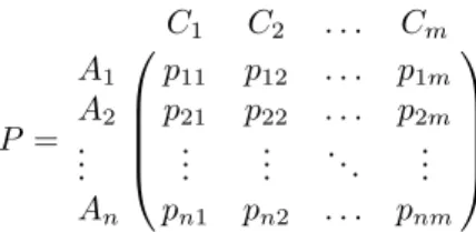
P = C1 C2 . . . Cm A1 p11 p12 . . . p1m A2 p21 p22 . . . p2m .. . ... ... . .. ... An pn1 pn2 . . . pnm
Figure 1: A decision matrix withnalternatives andm criteria.
feeders and a set of loads. The system is connected to the higher-level distribution system through a separation device. A node can be either a producer, a consumer, a prosumer, or a dispatcher. Each type of node is charac-terized by given attributes; in particular, producers and consumers, respectively, produce and require electricity, while prosumers may either produce or consume elec-tricity; finally, a dispatcher aims to dispatch the power produced by producers to consumers based on appro-priate efficiency criteria. All nodes in a graph-grid are connected to a dispatcher node. In this way, a lowest-level microgrid is modeled as a graph-grid including one producer node for each electricity source, one consumer node for each load, one prosumer node for each pro-sumer or energy storage, and one dispatcher node. On the other hand, a higher level (micro)grid is represented by a graph-grid that may include, besides the previous nodes, also prosumer nodes modeling lower-level mi-crogrids connected to the (micro)grid under analysis.
2. Multi-criteria decision making
A multi-criteria decision making (MCDM) problem is characterized by a goal, a set of criteria and a set of al-ternatives. Criteria and alternatives are calledelements. The goal consists in finding the best alternative with re-spect to all the criteria.
Most MCDM methods associate a weight with each criterion: usually weights are normalized to add up to one. Weights can be chosen by the expert or can result from a specific ranking technique.
An MCDM problem is usually described using a de-cision matrix. A dede-cision matrixP is ann×m ma-trix, where n is the number of alternatives and m is the number of criteria, as shown in figure 1. Each el-ementpijofP evaluates the performance of alternative
Ai with respect to criterionCj, wherei = 1,2, . . . , n
andj= 1,2, . . . , m.
2.1. Analytic Hierarchy Process (AHP)
Analythic hierarchy process (AHP) [9][10] decomposes a complex decision making problem into sub-problems which are simpler to solve. Since criteria might be divided into criteria and criteria into sub-subcriteria and so on, we will refer to a lowest-level sub-criterion as alowest sub-criterion. AHP organizes the problem as a hierarchy whose uppermost level con-tains the goal, intermediate levels contain criteria,
sub-criteria, etc., and the lowest level contains the alterna-tives.
AHP ranks criteria with respect to each other, with reference to their parent in the hierarchy. Alternatives are ranked according to each lowest sub-criterion. AHP generates a scale of priorities derived from pairwise comparisons. In practice, AHP firstly gives a structure to a complex problem and then let the decision maker understand which criteria are more important than oth-ers and which is the best alternative.
2.1.1. Description of the method
AHP requires to build a pairwise comparison matrix for each level of the hierarchy, by comparing elements shar-ing the same parent. Given two elements iand j the
Preference weightaij Explaination
1 Equally preferred
3 Moderately preferred
5 Strongly preferred
7 Very Strongly preferred
9 Extremely preferred
2, 4, 6, 8 Intermediate values (compromises)
Table 1: Saaty’s scale of preference.
result of a pairwise comparison is a coefficientmij
es-timating the preference ofioverj. Coefficient values, calledpreference weights, are usually expressed by us-ing Saaty’s scale of preference which connects quali-tative judgements to the first nine integer numbers, as shown in Table 1. Ifmij is the generic element of a
comparison matrixM, thenmii = 1andmij = 1/mji
for eachi, j = 1,2, . . . , n. A local weightwlocal i
ex-presses the importance of an elementi(either a criterion or an alternative) with respect to the others sharing the same parent in the hierarchy.
A matrixAis said to beconsistentifaij = aikakj,
where aij is the generic element of A and i, j, k = 1,2, . . . n. It has been proved [11] that the principal eigenvector is a representation of the priorities derived from a positive reciprocal pairwise comparison judge-ment matrix.
In order to obtainglobal weights, i.e., the weight of each element with respect to its uppermost ancestor in the hierarchy, the local weight of each element is multi-plied by the ones related to its ancestors in the hierarchy, until the uppermost level is reached. The results of these products are subsequently summed. Global weights of the elements in the lowest level of the hierarchy, i.e, the alternatives, represent the result of the decision making process. The decisional problem is solved by choosing the alternative having the greatest global weight.
2.1.2. Consistency check
Once local weights have been determined, we have to check if they reflect the expert’s judgements, obtained by pairwise comparisons. In other words, given ann×n pairwise comparison matrixA we need to verify how
much the ratios wlocali
wlocal j
derived from its principal eigen-vector differ from the estimatesaij with which the
ex-pert has filled the matrixA. In order to perform this check, AHP computes aconsistency index(CI) which expresses an overall difference between the valuesaij
andwilocal
wlocal j
, for eachi, j= 1,2, . . . , n.
Letλmaxbe the principal eigenvalue ofA. The
con-sistency index is defined as:CI , λmax−n
n−1 .Whenever the matrixAis consistent its principal eigenvalueλmax
is equal ton. Therefore, in the case of perfect
consis-n 3 4 5 6 7 8 9
RI 0.5245 0.8815 1.1086 1.2479 1.3417 1.4056 1.4499
Table 2: Random Index values obtained from 100000 n-order matrices.
tencyCI is equal to zero. As inconsistency increases, CIbecomes greater. AHP comparesCIwith arandom index(RI) which is obtained by calculating the mean of the consistency indexes of many reciprocal pairwise comparison matrices of the same order ofA, whose el-ements are randomly generated according to a uniform probability distribution. This comparison is performed by computing theconsistency ratio CR = CIRI. AHP considers a CR greater than 0.1 as unacceptable. If CR >0.1, the expert has to increase the coherence of his judgements by changing the entire set of estimates aij(or a part of it) untilCRbecomes lower than or equal
to 0.1. Table 2 shows the random indexes obtained from 100000n-order matrices.
2.2. Fuzzy AHP
2.2.1. Fuzzy sets and fuzzy numbers
Human judgements are usually affected by imprecision. Fuzzy sets deal with these situations [12]. The main con-cept of fuzzy set theory is that an elementxhas adegree of membershipµ(x) ∈ [0,1]in a fuzzy set [7][14]. A fuzzy number is a fuzzy set. We will use triangular fuzzy numbers. Givenl, m, u∈Rsuch thatl≤m≤u, a
tri-angular fuzzy number is a fuzzy setA = {(x, µ(x))}, wherex ∈ Randµ : R → [0,1]. The membership
functionµ(x)is: µ(x) = 0 if x < l∨x > u x−l m−l if l≤x≤m u−x u−m if m≤x≤u .
A triangular fuzzy number is indicated with A˜ = {l, m, u}. A further representation is based on the con-fidence level, i.e.,
˜
Aα= [lα, uα] = [(m−l)α+l,−(u−m)α+u], (1) for eachα∈ [0,1]. Given a fuzzy number (or, in gen-eral, a fuzzy set) the set{x|µ(x)>0}is calledsupport.
2.2.2. Fuzzy AHP procedure
Fuzzy AHP substitutes the Saaty’s scale of preference with a fuzzified version. Judgements are expressed by
triangular fuzzy numbers from˜1 to˜9 and the interval arithmetic is used to solve the fuzzy eigenvector [1].
More rigorously, let α ∈ (0,1], let A˜ be an n×
n matrix containing triangular fuzzy numbers ˜aαij = [aαijl, aαiju]and letx˜be a non-zeron×1vector contain-ing fuzzy numbersx˜i = [xαil, x
α
iu]. A fuzzy eigenvalue
˜
λis a fuzzy number solution toA˜x˜ = ˜λx.˜ In order to compute the eigenvector ofA˜connected with the prin-cipal fuzzy eigenvalue˜λ, fuzzy AHP defuzzifiesA˜. De-fuzzification is a process which maps a fuzzy set into a number. There are several ways to perform defuzzi-fication. Fuzzy AHP defuzzifies the matrixA˜by intro-ducing a coefficientζ∈[0,1], calledindex of optimism, with which it performs a convex combination of each element ofA˜, obtaining elements
ˆ
aαij =ζaαiju+ (1−ζ)aαijl. (2)
After defuzzifying the elements ofA˜, matrixAˆ= [ˆaαij]
is obtained. The eigenvector associated with the princi-pal eigenvalue ofAˆis calculated as in classic AHP.
2.3. Technique for Order of Preference by Similarity to Ideal Solution (TOPSIS) 2.3.1. Overview
The technique for order of preference by similarity to ideal solution (TOPSIS) is a multi-criteria decision mak-ing approach [2]. Consider a decisional problem char-acterized by n alternatives and m criteria. Let A = {1,2, . . . , n}be the set of indexes of the alternatives and letC ={1,2, . . . , m}be the set of indexes of the cri-teria. TOPSIS needs ann×mdecisional matrix whose generic rowi contains the performance the expert has estimated for the alternativesAiwith respect to each
cri-terionCj, wherei = 1,2, . . . , nandj = 1,2, . . . , m.
In addition, TOPSIS requires a vector containing the weights the expert has assigned to the criteria. Differ-ently from AHP, in TOPSIS the weights of the criteria and the weights of the alternatives with respect to each criterion are directly expressed by the expert. In order to select the best alternative, TOPSIS computes the ideal best and worst solutions to the problem: we will refer to them as theideal solutionand thenegative-ideal so-lution, respectively. The ideal solution and the negative-ideal solution are characterized, respectively, by the best and the worst performance attainable by all the alterna-tives with respect to each criterion. TOPSIS compares the alternatives with each other by computing the eu-clidean distance of each alternative from the ideal and negative-ideal solutions. The alternative to be chosen must have the shortest distance from the ideal solution and the farthest distance from the negative-ideal solu-tion.
2.3.2. Description of the method
The expert builds ann×mdecision matrixPsuch that nis the number of alternatives andmis the number of criteria, as shown in figure 1, whereAi is thei-th
judgement of the performance of thei-th alternative with respect to thej-th criterion.
Criteria are divided intocostcriteria andbenefit cri-teria. With reference to the benefit criterion Cj the
higher the elementpij, the greater the preference the
ex-pert assigns to alternativeAi over the others. On the
other hand, considering the cost criterionCk, the lower
the elementpikthe higher the preference the expert
ex-presses for Ai. Criteria may not have the same
im-portance, so TOPSIS considers a further vectorwT = (w1, w2, . . . , wm)containing the weights of the criteria such thatPm
j=1wj = 1.
By using the previous arguments, TOPSIS performs the following steps:
Step 1: construct the normalized decision ma-trix R.
The generic elementrijofRis:rij = pij pPn i=1p 2 ij .
Step 2: construct the weighted normalized deci-sion matrix V.
The generic elementvij ofV is:vij=wjrij. Step 3: determine the ideal and the negative-idealsolutions.
The two ideal alternatives (i.e., best and worst)A+ and A− are determined. LetJ be the set of in-dexes of the benefit criteria, and letJ0be the set of indexes of the cost criteria. A+andA− are com-posed by the elements:
v+j = max i∈A,j∈Jvij min i∈A,j∈J0vij v−j = min i∈A,j∈Jvij max i∈A,j∈J0vij. Step 4: calculate the separation measure.
Given an alternative Ai, i = 1,2, . . . , n,
TOP-SIS measures the separations of Ai from A+
and A−, indicated respectively with δi+ and δ−i by computing the euclidean distance, as fol-lows: δi+ = qPm j=1(vij−v+j)2 , δ − i = q Pm j=1(vij−v−j)2
Step 5: calculate the relative closeness to the ideal solution. For each alternativeAi, TOPSIS
computes the so-called closeness coefficient χ+i , defined as: χ+i = δ
−
i
δ+i+δi−. An alternativeAi is
closer toA+asχ+i approaches to 1.
Step 6: give a rank to the alternatives.
In this last step alternatives are ranked, according to the descending order ofχ+i .
The alternativeAk such that k = arg maxiχ+i is the
best.
3. Fundamentals of linear programming
A linear programming (LP) problem consists in mini-mizing or maximini-mizing a linear function, calledobjective function, subject to linear constraints. A point that sat-isfies all the constraints is called afeasible point and the set of all feasible points forms thefeasible region,
which geometrically represents a polytope described by the constraints of the problem. The objective function z : Rn → Rof an LP problem is a linear combination
of the decision variables xj whose coefficients arecj,
wherej = 1,2, . . . n. Therefore, the objective function isz=Pn
j=1cjxj.
Since mimimizing the objective functionz is equiv-alent to maximizing−z, from now on we will discuss minimization problems, without loss of generality.
Constraints are equations or inequalities of the form
Pn
j=1aijxj S bi,generated by linear combinations of the decision variables, whose coefficients are expressed by anm×nmatrixA.
An LP problem can be written in different equivalent forms through algebraic manipulations. An LP prob-lem is said to be in standard form if all the constraints are expressed by equations and all the variables are non-negative. EquationPn
j=1aijxj = bi is the i-th
con-straint,aij are the coefficients, and constraintsxj ≥0
are the non-negativity constraints, one for each variable. The fundamental theorem of LP states that if an LP problem whose feasible region is a polytope has a solu-tion, then it will occur in a vertex of the polytope, or on a line segment connecting two vertices.
Many techniques have been developed for evaluating the objective function value only in a subset of all the vertices: one of these approaches is the simplex method [4].
4. Efficient energy dispatching
Consider a microgrid represented by a directed graph havingnnodes andmarcs. Nodes can be active or pas-sive. A node is active (passive) if it provides (absorbs) energy. The sets of active and passive nodes will be in-dicated, respectively, withOandE, where O,E ⊂ N
andO ∩ E=∅.
A producerpis an active node with the following at-tributes:
• distance: is the distancedp ∈ R+ from the
dis-patcher node which the producer is connected to, expressed in kilometers;
• power: is the suppliable electrical power, measured in kW, represented by a negative integer;
• type of source: is the way by which the producer generates energy, e.g., fossil fuels, etc.;
• environmental impact: is the amount of pollutants (e.g., carbon dioxide, dioxins, etc.) released into the environment. The impact is supposed to be πp ∈ Π, where, e.g.,Π = {1,2,3,4,5} contains
increasing levels of contaminants emitted with en-ergy production;
• cost: is the costkp ∈R+per kWh of energy
pro-duced.
A consumerc is a passive node with the following attributes:
• power: is the power required by the consumer, measured in kW. It is represented by a positive in-teger or zero.
A prosumersis a node which produces or consumes electricity. At any instant, a prosumer is active if it can supply electricity, otherwise it is passive. A prosumer has all attributes of producers and consumers. As a pro-sumer produces using renewable sources, we assume a zero environmental impact.
A dispatcher is a node which neither consumes nor produces energy. Its task is dispatching the power avail-able in the active nodes to the passive nodes, according to criteria of efficiency. The set containing the dispatch-ers is indicated withD. Dispatchers are connected to each other through a nodeCCwhich is called thecentral controller. Like the dispatchers, the central controller neither produces nor consumes energy.
Each producer or consumer is connected to a dis-patcherDi∈ D,i∈ {1,2, . . . ,|D|}, through an arc. In
the case of a producer (consumer), the arc which con-nects it to a dispatcher has its head in the dispatcher (consumer) and its tail in the producer (dispatcher). Fur-ther, each prosumer is connected to a dispatcher through a pair of arcs: one directed to the dispatcher, the other directed to the prosumer. Finally, each dispatcher is con-nected to the central controller via a pair of arcs: one directed from the dispatcher to the central controller, the other directed in the opposite direction. Arcs are
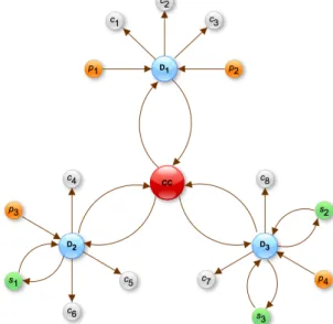
de-Figure 2: An example of a microgrid.
noted by ordered pairs. Given two nodesi, j ∈ N, the arc whose head isjand whose tail isiis(i, j). LetA1 be the set containing all the possible arcs connecting a dispatcher to the central controller and letA2be the set containing all the possible arcs connecting a dispatcher to an active or passive node. The setAcontaining the arcs of the microgrid is:A ⊆(A1∪ A2).
In compact notation, a microgrid is(N,A). Given a configuration of energy flow on the arcs of the grid, the optimization process of dispatching energy consid-ers the following criteria:
• environmental impact;
• cost of the energy;
• distance of supply;
• load level of the power lines.
The problem is addressed through an MCDM ap-proach using a hybrid method based on fuzzy AHP and TOPSIS: fuzzy AHP assigns the weights to each cri-terion and TOPSIS selects the best alternative. In our model, an alternative is a flow, i.e., a given configura-tion of energy flows on the arcs of the graph.
Of course, it is important to start with a reasonable number of good alternatives. To this aim, we use linear programming.
5. Strategy for generating alternatives 5.1. Mathematical model
Consider a microgrid(N,A). Given a nodei ∈ N let
N+(i) ={j ∈ N | ∃(i, j)∈ A}be the set of its suc-cessors andN−(i) ={j∈ N | ∃(j, i)∈ A}the set of its predecessors. The arcs of the graph can be described by ann×mincidence matrixE, whose generic element eihis:
eih=
−1 ifhis an outgoing arc from the nodei
1 ifhis an incoming arc to the nodei
0 otherwise.
(3) Each nodei ∈ N is characterized by an energy re-quirementbi ∈ Zmeasured in kW, which is the power
required (or suppliable) by the node. The central con-troller and the dispatchers have a zero energy require-ment.
Consider an active node i ∈ O connected to a dis-patcherDt, wheret ∈ {1,2, . . . ,|D|}. For the sake of
simplicity, in the following we will indicate withDthe dispatcherDt. The arc(i, D)∈ Awhich connectsito
the dispatcher is characterized by a distancediD ∈R+
from the dispatcher and an energy costkiD ∈ R+ for
each kWh provided by i. In addition, the arc (i, D)
is associated with minimum and maximum capacities ϕmin
iD andϕmaxiD of sustainable energy flow, whereϕminiD ,
ϕmax
iD ∈ Z+. On the contrary, if iis passive, the arc (D, i)∈ Ahas no energy cost, i.e.,kDi= 0, a minimum
and maximum capacitiesϕminDi andϕmaxDi of sustainable energy flow, whereϕminDi , ϕmaxDi ∈Z+.
To obtain alternatives, we generate sub-optimal solu-tions of an LP problem. Consider the objective function
aggregate costc:R2+→[0, γ]to minimize, defined as c(dij, kij) =γ αdij−dmin dmax +βkij−kmin kmax , (4) where(i, j) ∈ A,α∈[0,1],β = 1−αandγ ∈Z+.
kminandkmaxare, respectively, the minimum and
max-imum energy costs;dminanddmaxare, respectively, the
minimum and maximum distances of all the nodes from the dispatcher.
For each arc (i, j) ∈ A, let xij ∈ Z+ be the
en-ergy flow on the arc, and let ϕmin
ij andϕmaxij be,
(i, j). LetxT ∈
Zm+ be the vector containing a possi-ble configuration of energy flow on the arcs of the grid, and letϕTmin, ϕTmax ∈ Zm+ be, respectively, the vector of minimum flows and the vector of maximum sustain-able flows of the arcs. In addition, letcT ∈ Zm+ be the vector containing the aggregate cost of each arc of the grid. For the sake of simplicity, we denote bycij the
aggregate costc(dij, kij)of the arc(i, j). Finally, for
each nodei ∈ N, letbi be its energy requirement and
letb∈Zn
+be the vector containing the requirements of the nodes of the grid. Chosen a zero minimum energy flow on each arc and assuming that the total energy pro-duced by the active nodes meets the energy requirement of all the passive nodes, the LP model of the problem is:
min X (i,j)∈A cijxij X (i,j)|j∈N+(i) xij ≤ −bi ∀i∈ O X (j,i)|j∈N−(i) xji=bi ∀i∈ E X j∈N−(i) xji− X j∈N+(i) xij = 0 ∀i∈ D xij≤ϕmaxij ∀(i, j)∈ A xij≥0 ∀(i, j)∈ A X i∈O |bi| −X j∈E bj≥0. (5)
We are interested in sub-optimal solutions to the prob-lem (5) to be evaluated on the criteria the previous model does not take into account. We adopt a perturbation strategy in order to obtain a familyPof LP problems, so
that, once solved, each problem provides a sub-optimal solution to (5).
5.2. Perturbation of the model
Solving the problem (5) means to provide the amount of energy required by the passive nodes by saturating the arcs connecting active nodes to the dispatcher and having a low aggregate cost.
Given the optimal solutionx?to (5), we are interested
in the saturated arcs connecting active nodes to the dis-patcher, forming the setS. An arc(i, D)such thati∈ O
is said to be saturated if the flowxij on it equals the
en-ergy requirement|bi|of the active nodei.
The perturbation strategy is firstly based on desatu-rating, one by one, the saturated arcs, obtaining every time a new problem whose solution is a sub-optimal so-lution to (5). In this way, the flow units no longer pro-vided by the active nodes connected to a saturated arc, will be provided by active nodes having no saturated arc inS. In particular, considered an arc(i, D) ∈ S, the new maximum capacity of the arc is obtained as ϕmax0
ij =bεbic, ε∈[0,1),whereb cdenotes the floor,
i.e., the largest previous integer. By means of this strat-egy, at most|S|sub-optimal solutions to (5) can be ob-tained.
Subsequently, in order to increase the number of sub-optimal solutions to (5), we consider, in pairs, the arcs saturated by the optimal solution x? to the prob-lem P and simultaneously lower their maximum ca-pacity. More rigorously, given a pair of saturated arcs
{sh, sk} ∈ S, whereh6=k, the new maximum
capac-ity of the arcs forming the pair is obtained asϕmax0 sh =
bεbic,ϕmax 0
sk =bεbic,ε∈[0,1). By repeating the
pro-cedure for each pair of saturated arcs, additional sub-optimal solutions to the original problem (5) are ob-tained. In particular, by combining both previous ap-proaches, it is possible to obtain at most|S|+2(|S|−|S|!2)!
solutions.
6. Hybrid fuzzy AHP-TOPSIS approach for efficient energy dispatching
Once the alternatives have been generated by the per-turbation of the model, the system has to evaluate them in order to establish the best one, with respect to all the criteria. We propose the use of fuzzy AHP to prioritize the criteria. The alternatives are subsequently evaluated by means of TOPSIS. As said in Section 4, the consid-ered criteria are: the environmental impact; the cost of the energy; the distance of supply; the load level of the power lines.
First, the expert has to fill a matrixH˜ which com-pares the criteria with each other by means of a fuzzified Saaty’s scale of preference based on triangular fuzzy numbers from˜1to˜9, whose meaning is showed in Ta-ble 1, with the addition of uncertainty. The expert has also to express an index of optimismζabout the judge-ments as explained in Section 2.2.2. The system per-forms a defuzzification of the matrix H˜ according to equation (2), obtaining matrix Hˆ. Finally the system computes the principal eigenvectorwofHˆ, which con-tains the weights of the criteria.
For each alternative, the system computes the envi-ronmental impact, the cost of the energy, the distance of supply and the load level of the power lines. In particu-lar, given an alternativex, its environmental impactπx
is defined as: πx= P i|∃(i,D)∈AπixiD P i|∃(i,D)∈AϑixiD , ϑi = 1 ∀i|xiD6= 0 0 otherwise. (6) In addition, the cost of the energykxof the alternativex
is:
kx=
X
i|∃(i,D)∈A
kixiD. (7)
Further, the distance of supplydxis expressed by:
dx=
X
(i,j)∈A
dijxij. (8)
Finally, the load levellxof the power lines is defined as:
lx= 1−
P
(i,j)∈Aϕmaxij −
P
(i,j)∈Axij
P
(i,j)∈Aϕmaxij
, (9) where0< lx≤1.
Alternative Flow id p1D1p2D1 p3D2p4D3 s1D2 s2D3s3D3D2s1D3s2D3s3D1CC D2CC D3CC CCD1 CCD2CCD3 π k d l 1 9 14 9 13 4 0 9 0 4 0 0 4 0 2 0 2 2.9375 177 576 0.2833 2 8 14 9 14 5 0 9 0 4 0 0 4 0 3 0 1 2.9167 179 579 0.2833 3 7 14 9 15 4 0 9 0 4 0 0 4 0 4 0 0 2.8958 181 582 0.2833 4 6 14 9 16 4 0 9 0 4 0 0 4 0 5 0 0 2.8750 183 585 0.2833 5 9 13 9 14 4 0 9 0 4 0 0 4 0 3 0 1 2.9167 178 578 0.2833 6 9 13 9 14 4 0 9 0 4 0 0 4 0 3 0 1 2.9167 178 578 0.2833 7 9 11 9 16 4 0 9 0 4 0 0 5 0 5 0 0 2.8750 180 582 0.2833 8 9 10 9 17 5 0 9 0 4 0 0 4 1 6 0 0 2.8542 181 590 0.2875 9 9 9 9 18 5 0 9 0 4 0 0 5 2 7 0 0 2.8333 182 598 0.2917 10 9 14 8 14 5 0 9 0 4 0 0 3 0 2 0 1 2.8958 179 575 0.2792 11 9 14 7 15 4 0 10 0 4 0 0 3 0 2 0 0 2.8542 181 574 0.2750 12 9 14 6 16 5 0 9 0 4 0 0 2 0 2 0 0 2.8125 183 573 0.2708 13 10 14 5 17 5 0 10 0 4 0 0 1 1 2 0 0 2.7708 185 578 0.2708 14 9 14 4 18 5 0 9 0 4 0 0 0 2 2 0 0 2.7292 187 583 0.2708 15 8 13 9 15 4 0 10 0 4 0 0 4 0 4 0 0 2.8958 180 581 0.2833 16 7 12 9 17 5 0 9 0 4 0 0 4 1 6 0 0 2.8542 183 592 0.2875 17 6 11 9 19 5 0 9 0 4 0 0 5 3 8 0 0 2.8125 186 609 0.2958 18 9 13 8 15 4 0 9 0 4 0 0 3 0 3 0 0 2.8750 180 577 0.2792 19 9 12 7 17 5 0 9 0 4 0 0 3 1 4 0 0 2.8125 183 584 0.2792 20 9 14 9 17 2 0 7 0 4 0 0 2 0 2 0 0 2.8654 183 586 0.2750 21 9 14 9 19 1 0 6 0 4 0 0 2 0 2 0 0 2.8333 186 591 0.2708
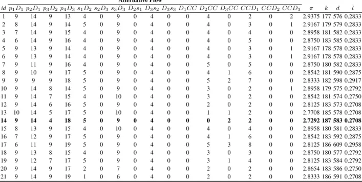
Table 3: Alternative flows with their performance values with respect to the criteria.
Ifnalternatives are generated, the system organizes them as rows of a matrixX, so as each row ofX con-tains the unities of flow for each arc of the grid. The performance values of each alternative with respect to the criteria are organized as rows of a matrixY, there-fore given a rowiofY, wherei= 1,2, . . . n, such row contains, respectively, the pollution level, the cost of the energy, the distance of supply and the load level of the power lines related to thei-th alternative. MatrixY is the decision matrix the system evaluates by means of TOPSIS, using the weights inw. At the end of the com-putation, the system returns the best alternative with re-spect to all the considered criteria.
7. Experiments
The system was implemented in MATLAB and was tested on a prototype microgrid consisting of four pro-ducers, eight consumers, three prosumers, three dis-patchers and a central controller, having the structure shown in figure 2.
Initially, we compared in pairs the criteria discussed in Section 4 so as to fill the fuzzy matrix needed by fuzzy AHP: ˜ H = E C D L E 1 ˜2 ˜3 ˜5 C ˜2−1 1 ˜5 ˜7 D ˜3−1 ˜5−1 1 ˜4 L ˜5−1 ˜7−1 ˜4−1 1 . (10)
The judgements inH˜ are used to prioritize the criteria in relation to a particular context, therefore they should be set by an expert. Nevertheless, we estimated the judgements according to common sense, providing them with an uncertainty expressed by triangular fuzzy numbers having a support equal to an interval with
length 2. The elements of the pairwise comparison ma-trixH˜ are taken by the functioncomputeWeights() as argument. The function performs a defuzzification according to equation (2), by using a further parameter ζ, i.e., the index of optimism we have described in Section 2.2.2. We chose ζ = 0.5, based on heuristic considerations. The returned consistency index was CI = 0.093, therefore the decision matrix H˜ was said to be consistent. In addition, the function re-turned the vector containing the weights of the criteria w = (0.434,0.381,0.132,0.053). At this point, the system asked the following parameters to be entered: the incidence matrix E of the network; the vector b of the energy requirements of the nodes; the vectors ϕmaxandϕmin of the maximum and minimum flows; the vector d of the distances between the connected nodes; the vector k of the energy costs. We entered the parameters according to a given order. Nodes were entered in groups, and the nodes in each group were in lexicographic order. Groups of nodes were composed, respectively, by consumers, producers, prosumers, dispatchers and finally the central controller. Arcs were entered in the following order: the ones connecting each dispatcher to the consumers, the ones connecting each producer to a dispatcher, the ones connecting each prosumer to a dispatcher and vice versa. Finally the system requires the arcs connecting each dispatcher to the central controller and the arcs connecting the central controller to the dispatchers. The parame-ters we inserted are summarized in the following: b= (8,12,7,2,3,5,15,7,−10,−15,−10,−20,−5,4,
−10);c= (0,0,0,0,0,0,0,0,2,3,2,4,2,2,3,0, . . . ,0); ϕmax= (20, . . . ,20);ϕmin= (0, . . . ,0);d= (3,4,2,
5,8,4,4,4,5,6,3,8,2,1,3,2,1,3, . . . ,3). For reasons of space, we omit the incidence matrix of the network. However, the incidence matrix can be easily obtained
according to equation (3), observing Figure 2.
By using the previous arguments, the system called the functiongetSubObtimalSolutions()which solved the optimization problem (5), finding the op-timal solution x?, by means of the simplex algo-rithm. The optimal solution of the problem wasx? = (8,12,7,2,3,5,15,7,10,15,10,13,5,0,10,0,4,0,0,5
,0,2,0,3). The system then began to perturb the model lowering the maximum capacities of the sat-urated arcs, firstly one at a time, successively in pairs, obtaining suboptimal solutions, i.e., the al-ternatives to be evaluated. For each alternative, the system calculated the values of the criteria, ac-cording to equations (6-9), by calling the function evaluateAlternativesOnCriteria(). In Ta-ble 3 we have summarized the suboptimal solutions. In the header of the table there are, from left to right, an identifieridof the alternative, and the arcs connecting, respectively, producers to dispatchers, prosumers to dis-patchers, dispatchers to the central controller and central controller to the dispatchers. Note that, for reasons of space, arcs are represented without the arrow. For ex-ample, the arcp1D1represents the arcp1 → D1. The header of the table is terminated with the symbols de-noting the criteria, i.e., the pollution levelπ, the cost of the energyk, the distance of supplydand the load level lof the power lines. We have also omitted the first eight columns which would contain the incoming flows of the consumers. Such flows are the same for each alternative, i.e.,{8,12,7,2,3,5,15,7}.
As last step, the system passed the alternatives shown in Table 3 to the function rankAlternatives() which, by means of the TOPSIS algorithm and using the weights inw, chose the alternative 14 as the best one. In Table 3 the best alternative is represented in bold.
8. Conclusions
In this paper we presented a new approach based on multi-criteria optimization and decision making to opti-mize the energy dispatching in smart (micro)grids. The optimization method we have proposed is based on four criteria: environmental impact, energy cost, distance of supply, and load level of the power lines. The problem has been modeled by means of linear programming, by arbitrarily considering two of the four criteria, i.e., the distance of supply and the cost of the energy. By mod-ifying the maximum flow constraints of the problem it has been possible to generate sub-optimal flows. Such flows have been subsequently evaluated on the criteria the LP model does not take into account, by means of a hybrid multi-criteria decision making approach based on fuzzy AHP and TOPSIS. Fuzzy AHP has been used to associate a weight with each criterion according to the judgements of an expert, in order to obtain a vector of weights so as to prioritize the criteria. Subsequently, TOPSIS has been used to select the best configuration of flow among the available ones, with respect to all the criteria.
We believe the proposed approach is interesting since
it is based on evaluations of the importance of the crite-ria which can be expressed with different levels of uncer-tainty and vagueness. In addition, an MCDM approach allows to manage the problem quite easily thanks to the use of pairwise comparison matrices for the prioritiza-tion of the criteria and an evaluaprioritiza-tion of the alternatives simply based on the performance they attain on each cri-terion.
The proposed approach can be extended by consid-ering further criteria and guiding the generation of the alternatives according to different strategies of perturba-tion, to be used even in parallel. Finally, it is also possi-ble to extend the model to deal with larger grids, maybe composed by a potentially high number of microgrids.
References
[1] D. Ruan C. Kahraman, U. Cebeci. Multi-attribute comparison of catering service companies using fuzzy ahp: the case of turkey. International Jour-nal of Production Economics, 87:171–184, 2004. [2] Kwangsun Yoon Ching-Lai Hwang. Multiple
at-tribute decision making. Springer-Verlag, 1981. [3] David Cornforth. The role of microgrids in the
smart grid.Journal of Electronic Science and Tech-nology, 9(1):9–16, March 2011.
[4] George B. Dantzig. Linear Programming and Ex-tensions. Princeton University Press, 1965. [5] C. Marnay G. Venkataramanan. A larger role
for microgrids. IEEE Power Energy Magazine, 5(4):78–82, May/June 2008.
[6] B. Lasseter. Microgrids (distributed power genera-tion). InProceedings of IEEE Power Engineering Society Winter Meeting, volume 1, pages 146–149, Ohio, USA, February 2001.
[7] C. V. Negoi¸t˘a. Expert systems and fuzzy systems. Benjamin-Cummings Publishing Co., 1985. [8] Reza Iravani Chris Marnay Nikos Hatziargyriou,
Hiroshi Asano. Microgrids. Power and Energy Magazine, IEEE, 5(4):78–94, August 2007. [9] Thomas L. Saaty. The analytic hierarchy process:
Planning priority setting. McGraw Hill, 1980. [10] Thomas L. Saaty. How to make a decision: The
analytic hierarchy process. European Journal of Operational Research, (48):9–26, 1990.
[11] Thomas L. Saaty. Decision-making with the ahp: Why is the principal eigenvector necessary. Euro-pean Journal of Operational Research, 145:85–91, 2003.
[12] L. A. Zadeh. Fuzzy sets.Information and Control, 8(3):338–353, 1965.
[13] Furong Li Zhenjie Li, Yuan Yue Yuan. Evalu-ating the reliability of islanded microgrid in an emergency mode. InUniversities Power Engineer-ing Conference (UPEC), 2010 45th International, pages 1–5, 2010.
[14] H. J. Zimmermann.Fuzzy set theory and its appli-cations. Kluwer, 1985.