Supplementary Materials for

(1)

advances.sciencemag.org/cgi/content/full/6/42/eabc3204/DC1

Explainable and trustworthy artificial intelligence for

correctable modeling in chemical sciences

Jinchao Feng, Joshua L. Lansford, Markos A. Katsoulakis*, Dionisios G. Vlachos* *Corresponding author. Email: [email protected] (M.A.K.); [email protected] (D.G.V.)

Published 14 October 2020, Sci. Adv. 6, eabc3204 (2020) DOI: 10.1126/sciadv.abc3204

This PDF file includes:

Sections S1 to S8

Figs. S1 to S8

Tables S1 to S5

References

(2)

Glossary and Outline of Methods

1. Model Uncertainty for General Probabilistic Models

• Model Misspecification=η orηl, where

η=R(Q||P)

the KL divergence/relative entropy between an alternative modelQand baseline modelP.

• We define theambiguity sets which contains all the alternative modelsQto the baseline modelP, e.g. the ambiguity set for model uncertainty

Dη ₌_{_Q_:_R₍_Q_||_P₎_≤_η_}

This is an infinite dimensional set of probabilities containing all possible models η-“close” to P in Kullback-Leibler (KL) divergence, including the unknown “real” model.

• Model Uncertaintyfor the (Quantity of Interest) QoI f and model misspecification η:

I±(f, P;η) = max/min

Q∈Dη E

Q[f]−EP[f]

the worst case scenarios for the bias of predictions of QoIf when we perturb the baseline model P

to an alternative modelQunder model misspecificationη (i.e.,Q∈ Dη_).

Similarly we can define therelative model uncertaintyby normalizing the model uncertainty with the QoIEP[f]: I±(f, P;η) EP[f] = max/min Q∈Dη E Q[f]−EP[f] EP[f]

2. Model Uncertainty for Probabilistic Graphical Models

• For each Conditional Probability Distribution (CPD) we define the analogousCPD misspecifica-tion:

ηl=EP[R(Ql(·|PaXl)||Pl(·|PaXl))]

the averaged KL divergence/relative entropy between an alternative modelQl and baseline modelPl

with the same parents PaXl. Alternatively we can also define for convenience,

ηl= max

Pa_XlR(Ql(·|PaXl)||Pl(·|PaXl)).

• We define the ambiguity set for model uncertainty guarantees as

Dηl

l ={Q:R(Q(Xl|PaXl)||P(Xl|PaXl))≤ηlfor all PaXlof modelP , Q(Xj|PaXj)≡P(Xj|PaXj) for allj6=l}

which is an infinite dimensional set containing all possible models (parametric/non-parametric)

ηl-“close” to P at the l-component in Kullback-Leibler (KL) divergence, i.e., we only perturb the

l-component of P under the model mis-specification ηl and keep the remaining CPD and graph

structure (usually here a DAG) fixed.

• Model Uncertainty Guaranteesforl-node perturbationηl: J_l±(f, P;ηl) = max/min

Q∈D_lηl

EQ[f]−EP[f]

the worst case scenarios for the bias of predictions of QoIf when we perturb only the l-component of the baseline modelP to an alternative modelQunder model mis-specificationηl(i.e.,Q∈ D

ηl

(3)

Similarly we can define the relative model uncertainty guarantees by normalizing the model uncertainty guarantees with the QoIEP[f]:

J±(f, P;ηl) EP[f] = max/min Q∈Dlηl EQ [f]−_EP[f] EP[f]

• PGM Ranking Indexof model uncertainty:

J_l±(f, P;ηl) P kJ ± k(f, P;ηk) .

The Ranking Index allows to interpret, reevaluate and improve the baseline PGM modelP by com-paring the contributions of each CPD to the overall uncertainty of the QoIf.

(4)

1

ORR Chemistry and the Equilibrium Method

Fuel cells are an optimal choice for chemical energy storage as they have high energy and power densities (55,

56) and can make use of existing infrastructure for fuel storage and transportation via liquid hydrogen carriers (57) or direct alcohol fuel cells (DAFC) (58–60). The oxygen reduction reaction (ORR) is an important electrochemical reaction most often associated with the cathode side of a fuel cell. Regardless of the fuel used in the anode side, a complete fuel cell device will almost always involve oxygen as it is readily available. Although fuel cells are already three times as efficient as the internal combustion engine used in cars today (61), the ORR still requires high overpotentials (33, 62). The electrochemical field has been very active in addressing this issue by investigating transition metal alloys of Pt to increase reaction rates, thereby lowering the necessary overpotential (63). Much of this work has made use of volcano curve screening for catalyst activity (9). Still, an industry standard material consisting of non-noble metals has yet to be developed. Development of an inexpensive catalyst is necessary if fuel cells are to be a viable alternative to the internal combustion engine. The purpose of this work is to isolate and quantify sources of error in the volcano curve used in determining the optimum oxygen binding energy (∆G∗_O) for maximizing the activity (reaction rate) of the metal-catalyzed ORR, which will be discussed in more detail after introduction of the relevant chemistry. We choose to study ORR in acidic media because, even though activity in alkaline electrolytes is comparable for the ORR, activity of the anodic hydrogen oxidation reaction (HOR) is greatly diminished in the presence of alkaline electrolytes (64, 65).

There is support in the scientific literature that the ORR reaction rate depends on two competing elementary reaction steps (66). In acidic media, these two steps are surface hydroperoxyl (OOH*) formation from molecular oxygen (O2) as shown in Equation (1), and water (H2O) formation from desorption of surface hydroxide (OH*)

which can be found in Equation (4) (7, 35). The rate of the former is enhanced by increasing catalyst binding strength and the rate of the latter is enhanced by decreasing catalyst binding strength. Both of these adsorption and desorption steps also involve the consumption of an electron and a proton. The complete mechanism, as is often proposed (7, 36, 37), involves four electron consuming steps: (1) solvatedO2 forming adsorbed OOH at

a free catalyst site, (2) adsorbed OOH forming adsorbed atomic oxygen (O) and solvatedH2O, (3) adsorbed O

forming adsorbed OH, and (4)H2Oformation and regeneration of the free catalyst site from adsorbed OH. The

four electrochemical steps are illustrated below

∗+O2+H++e− →OOH∗ (1)

OOH∗+H++e−→O∗+H2O (2)

O∗+H++e−→OH∗ (3)

OH∗+H++e−→ ∗+H2O. (4)

Here, * represents an unoccupied metal binding site and, when placed next to a species (such as OOH*), refers to the species in the adsorbed state (chemisorbed to the metal). H+ ₊_e− _{signify proton and electron consumption}

associated with an elementary step.

The reaction rate of each elementary step is determined using statistical mechanics and harmonic transition state theory (9). The first step to determining the reaction rate is calculating the Gibbs free energy (G) of each species

G=EDF T +ZP E+

Z 298

0

GdT +Esolv. (5)

In Equation (5),G is the sum of the 0 K electronic energy in vacuum calculated from DFT (EDF T), the zero

point energy (ZP E), the temperature effects to the Gibbs energy (R298

0 GdT), and contributions from solvation

(Esolv_{) in liquid water (}_H

2O(l)). The ORR under operating conditions occurs at finite temperatures in an

aqueous environment which is why we must account for temperature and solvation effects. All temperature effects are taken to 298 K.

All surface species are referenced to hydrogen (H2) and H2O(l) to avoid DFT error in molecular oxygen

(5)

is referenced to the standard hydrogen electrode (SHE) (7,67). The Gibbs energies of formation (∆G) forO∗,

OOH∗, O2, and OH* are then

∆GO =GO∗+G_H 2−G∗−GH2O(l) (6) ∆GOOH=GOOH∗+ 3/2GH2−G∗−2GH2O(l) (7) ∆GO2 := 4.92eV (8) ∆GOH =GOH∗+ 1/2G_H 2−G∗−GH2O(l). (9)

As mentioned previously, GO∗, G_OOH∗, andG_OH∗ refer to surface species and G_∗ indicates the energy of the

surface without the presence of an adsorbate.

Steps (1) and (4) are often the only rate-limiting steps for the ORR (7). Thus, we are only interested in the Gibbs energies of reaction (∆G) for steps (1) and (4). ∆G1 and ∆G4 are determined using the previously

mentioned formation energies as follows

∆G1= ∆GOOH−∆GO2 (10)

∆G4=−∆GOH. (11)

Transition states of charge transfer reactions, especially those involving an electrode, are difficult to calculate. Furthermore, the methods that have been used to quantify the energy barriers of OOH* formation and OH* desorption reveal small energy barriers on platinum (Pt) and Pt-bimetallic alloys (68–70). For this reason we chose an equilibrium-based method, discussed in previous work(38), to determine the rate from

rate∝e−max[∆G1,∆G4]/kBT ₍₁₂₎

wherekBis Boltzmann’s constant andTis the temperature. This particular application of the Sabatier principle

is the result of combining the generally-accepted theory that the rate of a reaction at low coverage is equal to the reaction rate of the rate-limiting step(9, 71) and the result of transition state theory(9) that reveals that the rate of an elementary step is equal to the quantity of the reacting speciesitimese−∆G‡_i_{, where ∆}_G‡

i is the

difference in Gibbs energy of the transition state and initial state of elementary stepi. As we use an equilibrium method, we substitute the final state Gibbs energy of reaction step ifor that of the transition state. We scale the rate with the experimentally measured rate on Pt(111) at 0.9V relative to SHE (7)

rate= 1.357×10−15[mA/atom]/e−max[∆GP t1 ,∆G

P t

4 ]/kBT _×_e−max[∆G1,∆G4]/kBT ₍₁₃₎

and ∆GP t1 and ∆GP t4 refer to the DFT-calculated ∆Gfor steps (1) and (4) of the reaction network on Pt(111).

Additional details of this calculation are presented in the next Section.

2

Workflow for Deterministic Modeling in Materials Prediction

In this Section we discuss the existing deterministic workflow in constructing the ORR volcano curve. In subsequent Sections and in the Main Text we demonstrate how to augment this “human” workflow in order to incorporate data, correlations, causation relations, and expert knowledge along with modeling uncertainties, using probabilistic AI methods, and specifically graphical models.

First, we seek to identify hidden dependencies in our model. We note that the log of competing limiting reaction rates depend on an easy-to-calculate chemical descriptor (9), and correlations between reaction rates of OOH∗ and OH∗ withO∗ have been demonstrated previously (72). For our model, ∆GO is treated as the

descriptor for ORR activity because it is fast to calculate through first-principles, has the relatively few potential energy minima, and its energy scales with ∆GOOH and ∆GOH. Functional relations of the values of GOOH∗

and GOH∗ in terms of the values ofG_O∗ have previously been suggested as a materials prediction tool for the

ORR reaction (73, 74). Equations (14) and (15) show the linear dependence of ∆GOOH and ∆GOH on ∆GO

with slopeαand interceptβ, namely

(6)

∆GOH =αOH∗∆G_O+β_OH∗. (15)

Due to valance of OOH∗ and OH* being half that ofO∗, αfor both species is approximately equal to 0.5 (6,

30), although this scaling can vary with solvation (72,75). The linear relations (14) and (15), along with their intersection for determining the optimal ∆GO are shown in Figure 1c of the Main Text, where the intersection

of the solid lines gives rise to the well-known deterministic volcano curve (9).

Figure S1: Gibbs energies for OOH adsorption (blue) and OH desorption (red). Shown are results using DFT computed values ∆GOOH and ∆GOH (circles) calculated using Eqs. 6-9 and regressed values using Equations

(14) and (15) (lines) for adsorption on close packed surfaces of fcc and hcp metals.

The optimal ∆GO (∆G∗O) is identified from the intersection of the solid red and blue curves in Figure 1c of

the Main Text. This intersection corresponds to the maximum of the function min(−∆G1,−∆G4)

Optimal ∆GO:= argmax [ min{−∆G1,−∆G4}]. (16)

The maximum rate corresponds to the optimal ∆GO,

maximum rate = e−max(min{−∆G1,−∆G4})_×1.357×10

−15 mA atom e −max(∆GP t₁ ,∆GP t₄ ) kB T . (17)

All possible rates can be found from the set of max(∆G1,∆G4) using Equation (13), namely

{rates}=e−max{∆G1,∆G4}_×1.357×10 −15 mA atom e −max(∆GP t₁ ,∆GP t₄ ) kB T . (18)

The natural log of the rate computed from Equation (18) forms a volcano plot as shown in Figure 3a of the Main Text. In order to reduce the model error and correct our baseline model, as explained in the Main Text, DFT data from bimetallics was added in Figure 5a of the Main Text.

(7)

3

Probabilistic Models for DFT Errors and Experimental

Measure-ments

In determining the maximum ∆GO, the model, as discussed above, is deterministic. There are known errors in

the experiments, DFT, and the regression used to determine the optimum point. Therefore, it is appropriate to formulate the model in a stochastic manner such that ∆GO, ∆GOOH and ∆GOH as calculated from DFT are

treated as random variables, given a specific experimental Gibbs formation energy (∆GO(Exp)).

Except for the regression parameters (αOOH∗, β_OOH∗, α_OH∗, β_OH∗), which will be discussed later, the

relevant errors used in generating the probability distributions are found in Table S1.

Table S1: Errors in experimental and DFT values used in the model Parameter Mean Error [eV] Standard Deviation [eV]

∆GO(Exp) 0 0.1091 ∆GOH(Exp) 0 0.0805 ∆GOOH(Exp) 0 0.0805 ∆GO(DF T) -0.0754 0.3213 ∆GOH(DF T) -0.0222 0.1881 ∆GOOH(DF T) -0.0222 0.1881 Esolv H2O 0 0.0156 Esolv O∗ 0 0.0312 E_OHsolv∗ 0 0.0677 Esolv OOH∗ 0 0.0732

There are two kinds of error in the experimental measurements of ∆GO(Exp), ∆GOH(Exp), and ∆GOOH(Exp)

arising from (1) differences in repeated measurements by the same individual/group and (2) differences in measurements performed by different individuals/groups. This partitioning becomes especially important when dealing with small data. Repeated calorimetry and temperature programmed desorption (TPD) measurements for the dissociative adsorption enthalpy of O2 on Ir(111), Rh(111), Pt(111), Pt(110), Ni(100), Ni(110), and

Ni(111) surfaces by the same individuals show an average standard error in the mean of 0.109 eV/atom with a standard deviation of 0.070 eV/atom (76–81). Adsorption enthalpy measurements by multiple research groups are only available for Pt(111) and show a standard deviation of 0.046 eV/atom (76, 82–84) which is less than the average reported standard errors suggesting systematic errors between groups do not vary. We take 0.109 eV/atom as the standard deviation in ∆GO(Exp) since it is more representative of the error across different

metal surfaces.

Standard errors are not provided for any OH∗ experimental chemisorption enthalpies. There do exist, however, multiple measurements on Pt(111) by different research groups allowing us to estimate source (2) error (85–88). The standard deviation of ∆GOH(Exp) on Pt(111) is 0.0805 eV/atom, which is similar to the

average standard error in ∆GO(Exp) from several surfaces. We therefore take 0.0805 eV/atom as the error in

∆GOH(Exp). Because experimental values do not exist for OOH∗ chemisorption, we also take 0.0805 eV/atom

as the error in ∆GOOH(Exp). The error inOH∗ chemisorption is a good approximation for the error inOOH∗

chemisorption because both species bind to the surface through an oxygen atom that has a valency of one.

The error in ∆GO is defined as the error in theO2 enthalpy of dissociative adsorption minus half the error

in theO2 (gas) bond dissociation enthalpy (89), as outlined in Equation (19).

Error in∆GO _eV atom := Error in∆H_ads,ODF T −1 2Error in∆H DF T O2(g) . (19)

We subtract the error in bond dissociation enthalpy because ∆GO is referenced to H2 and H2O(l) to avoid

the error in the DFT calculated O2 bond dissociation enthalpy. We note here that all errors in chemisorption

energies are calculated at 300 K because that was the temperature listed for the experimental chemisorption data from literature. All other calculations are done at 298 K.

(8)

The errors in the DFT O∗ adsorption enthalpy andO2 (gas) bond dissociation enthalpy is the DFT bond

dissociation enthalpy, found by subtracting the DFT calculated value and that found experimentally, are outlined in equations (20) and (21) respectively,

Error in∆H_ads,ODF T =

∆H_ads,ODF T −∆H_ads,OExp

, (20) Error in∆H_ODF T 2(g)= ∆H_ODF T 2(g)−∆H Exp O2(g) , (21) where ∆H_ODF T 2(g)= ∆H_ODF T 2(gas)−2∆H DF T O(gas) . (22)

Experimental measurements forO2chemisorption were available for 16 metal surfaces (77–80,84,90–97). The

error in ∆GOhas a mean value of -0.0754 eV/atom with a standard deviation of 0.321 eV/atom and a standard

error in the mean of 0.0803 eV/atom. We find through our calculations that the DFT error in H2 and H2O

formation energies is small. All errors passed the Kolmogorov-Smirnov test (98) for normality, however, due to the lack of data samples and physical similarities between specific data points (such as number of d-electrons), modeling the error with Gaussian distribution is imperfect, so we must consider the impact of model uncertainty in our QoI predictions.

The error in ∆GOH is defined as the error in the OH adsorption enthalpy. The DFT calculatedOH(g) energy

used to determine the error inOH chemisorption energy is referenced to 1

2O2(g) + 1

2H2(g) via the experimental

heat of formation at standard state forOH(g) (87) to avoid DFT error in theO2(g) dissociation enthalpy.

The error in the enthalpy of adsorption is the difference between our DFT calculated adsorption enthalpies (∆HDF T

ads,OH) at 300 K and the relevant experimental enthalpies (∆H Exp

ads,OH) such that

Error in∆H_ads,OHDF T =

∆H_ads,OHDF T −∆H_ads,OHExp

, (23) and Error in∆GOH(DF T) _eV atom :=Error in∆Hads,OHDF T . (24)

Experimental measurements for OH chemisorption were available on 5 metal surfaces (86, 97, 99, 100). The error in ∆GOH has a mean value of -0.022 eV/atom with a standard deviation of 0.188 eV/atom and a standard

error in the mean of 0.084 eV/atom. For reasons discussed previously, we take these same values as the error in ∆GOOH.

The last error we discuss isEsolv_{. Our value for solvation energy of} _H

2O(l) comes from experiment (101)

and is assumed to have no error, as it is computed from standard thermodynamic tables and is the negative vaporization energy per molecule of water at constant temperature and pressure. The DFT calculated values of Esolv _{are for ∆}_G

O, ∆GOOH and ∆GOH. Solvation energies from DFT were determined by computing the

adsorption energy on Pt(111) in the presence of two layers of explicit water molecules in a honeycomb pattern (38) (∆Eaqu_ads) and subtracting from it the computed adsorption energy on Pt(111) without water (∆E_adsvac) where

∆E_adsaqu=E_slabaqu₊_adsorbate−Eaqu_slab, (25) and

∆E_adsvac=E_slabvac₊_adsorbate−E_slabvac, (26) and

Esolv = ∆E_adsaqu−∆E_adsvac. (27) There are no reported experimental solvation values to obtain a mean error. Meng et al. have shown that the DFT-computed value of adsorption energy of H2O on Pt(111) greatly depends on solvation but does not

change significantly when including two or more explicit layers of water molecules (50). Meng et al. computed adsorption energies for nine unique conformations of water molecules consisting of at least two water layers up to six water layers, resulting in mean adsorption energy of -0.588 eV and a standard deviation of 0.0156 eV per water molecule. After applying our calculated solvation contributions, errors in ∆GOH on solvated

(9)

Pt(111) and Pt(100) are 0.049 eV/atom and -0.009 eV/atom, respectively, when compared to experimentalOH

chemisorption energies; this suggests our solvation calculations for OH are accurate. These were the only two materials for which experimental chemisorption data was available in a solvated environment. The volcanoes in Figure 1c and 5a of the Main Text include solvation because industrially relevant reactions take place in a solvated environment.

Calculated errors for parameters other than the regression coefficients are summarized in Table S1. All errors passed the Kolmogorov-Smirnov test of normality (results shown in Table S4) and are therefore taken to be normally distributed. Table S2 shows that after hexagonal water bilayers the solvation energy is converged

with scatter around the mean value as there is no longer a systematic decrease or increase in solvation energy. This convergence is consistent with calculations by Meng et al. (50).

Table S2: Solvation Energies forO∗,OH∗, and OOH∗

Hexagonal Water Layers O∗ Solvation Energy [eV] OH∗ Solvation Energy [eV] OOH∗ Solvation Energy [eV] Two 0.01005 0.2161 -0.0678 Three 0.01364 0.1760 -0.1024 Four 0.03903 0.1637 -0.2285 Five -0.03588 0.1476 -0.0847

Although in many instances discussed in this Section errors passed the Kolmogorov-Smirnov test (98) for normality, the lack of sufficient data samples implies that modeling the error with Gaussian distributions is imperfect. Additional uncertainties arise from imperfect physico-chemical modeling, therefore we necessarily need to consider the impact of model uncertainty in our QoI predictions. We discuss such mathematical and computational methods in Sections 6-9.

4

Learning the Chemical PGM

The PGM is a graphical approach to model design where a series of interconnected vertices encode knowledge into its structure. These vertices represent quantifiable variables and are connected by edges which represent probabilistic interactions between variables (25). PGMs are an important class of methods for probabilistic mod-eling and inference in machine learning and constitute the mathematical foundation of the work on uncertainty in AI. They are used in medical diagnostics, natural language processing, computer vision, robotics, compu-tational biology, and cognitive science (20, 102–106). Their general mathematical formulation, introduced by the seminal work of J. Pearl (107) developing complex probabilistic models and corresponding algorithms for inference, revolutionized the field of AI. The material presented here will be divided in three parts: Gaussian Bayesian networks for ORR PGM, structure learning and parameter learning.

4.1

Structure Learning and Parameter Learning

General Methodology: First, we describe how to build the PGM for a physico-chemical system in general in two steps: learning the PGM graph structure (structure learning), and learning the probability density functions for the PGM (parameter learning). For structure learning, we first construct correlations(12, 13) between physico-chemical mechanisms, related parameters or any available descriptors to provide the graph structure of the PGM (graph nodes) and their connectivity. Subsequently, we determine the causal directions on the graph based on expert knowledge on the particular system, and statistical dependency learned from available data (41). For parameter learning, we build the functional forms of CPDs, in the mathematical definition of the PGMs, for each graph node by statistical fitting available sparse data to probabilistic parametric models with maximum likelihood estimator (MLE) or Bayesian methods (25); Gaussian networks shown in Section 4.2 and non-parametric models such kernel density estimators (25) are examples of this methodology.

Next we demonstrate this general methodology in a specific example where we build the ORR PGM, by implementing two main steps discussed above.

(10)

Structure Learning from (sparse) data and expert knowledge: Here we will present the details of

building the graphical model for ORR starting with the data in Figure 1c of the Main Text. In order to simplify

our notation, we use the following conventions for our random variables:

∆GO(DF T)=x , ∆GO =x0, −∆G1=y1, −∆G4=y4, (28)

where ∆GO is the true (unknown) value of the oxygen binding energy. We build the PGM in Figure 2 of the

Main Text via the following steps:

(a) Construct a random variablexfrom the DFT data for the oxygen binding energy given the real unknown valuex0;

(b) Use correlation analysis to discover statisticalcorrelations between the DFT (quantum calculation) data

xand theyi’s.

(c) Selectxas a descriptor (for the reasons discussed in Section 2), and therefore, establish acausal relationship

betweenxandyi, i.e. we create the corresponding directed edges in the graph, see Figure 2 of the Main

Text.

(d) Use a statistical dependency test (108), to show that y1 = −∆G1 and y4 = −∆G4 are conditionally

independent givenx= ∆GO(DF T), see Figure 2 of the Main Text.

We use a kernel-based conditional independence test (109, 110) for the null hypothesis H0: yi are

inde-pendent givenx, the resulting p-value equals 0.174 at 5% significance level, which in turn indicates that we can not reject the null hypothesis, i.e. it is reasonable to assume thatyiare conditionally independent

givenx.

(e) Model the residual random error in correlation (random variableωci).

(f) Model as random variables and incorporate in the PGM different kinds of errors in x and yi (given by

expert knowledge) from different sources:

– ωei: error in experimental data,

– ωdi: error of quantum calculations with respect to experimental values,

– ωsi: error due to solvation effects calculated via DFT.

We add these random variables into the PGM and build the connection/arrows with the corresponded random variablexoryi.

(g) Finally, we add the QoIs, ∆G∗

O=x∗0andr∗, whose evaluations depend on the values ofy1 andy4for each

x0 due to physics knowledge.

The steps above allo us to build part of the network structure withx= ∆G0,y1=−∆G1andy4=−∆G4using

a constraint-based method (41), which selects a desired structure based on constraints of dependency among variables. We note that we combined data from DFT computations (x, yi,ωci,ωdi,ωsi, depicted inblue), with

experimental data (ωei,ωdi, depicted ingreen); we fused these heterogeneous experimental and computational

data by taking advantage of the PGM formulation in Figure 2 of the Main Text.

Once the volcano curve between x and yi is constructed, we obtain a prediction for the optimal oxygen

binding energy x∗_O and optimal reaction rate r∗ using physical modeling, i.e. that the optimal oxygen binding energy is identified when the two reaction energies are equal and the optimal reaction rate is proportional to exp{max[min[y1, y4]]/(kBT)}.

Parameter Learning from sparse DFT data: Once we have obtained the structure of the graph from the previous step, we then learn the model

P(X|θ) =Y

i

P(Xi|PaXi, θXi|PaXi)

(11)

(a) First, we select a parametric family for models P(Xi|PaXi, θXi|PaXi). For the ORR example, we select as

our parametric family of PGMs, a family of Gaussian Bayesian Networks (GBN). In this case the CPDs take the form p(Xi|PaXi, θXi|PaXi) =N(βi0+β T i PaXi, σ 2 i). (29)

In other words, for parents PaXi ={Xi1, . . . , Xim} ⊂ {X1, . . . , Xn}, we have θXi|PaXi = (βi0, βi, σi)

T_{, where} βi = (βi,i1, . . . , βi,im), and assume varianceσ

2

i which does not depend on PaXi for all i= 1, ..., n. We refer to

Section 4.2 below for full details.

(b) Here we use Maximum Likelihood Estimation (MLE) to identify the parametersθthat fit best the available data. O course we can also employ a Bayesian approach instead of MLE, see for instance (25) for the case of PGMs. In the MLE step, we take advantage of the Global Likelihood Decomposition (25),

L(θ;D) =Y i Li(θXi|PaXi|D) = Y i Y m P(xi[m]|PaXi[m];θXi|PaXi) (30)

where L(θ;D) is the likelihood given dataD={ξ[1], . . . , ξ[M]} see Figure 1c of the Main Text; noting that

logL(θ;D) =X

i

logLi(θXi|PaXi|D), (31)

we observe that if we assume thatθXi|PaXi are disjoint, i.e. that each conditional probability density,P(Xi|PaXi,

θXi|PaXi), is parametrized by a separate set of parameters that do not overlap (this is a general assumption

The formulas, (31) and (32), imply that we can “divide and conquer” our overall learning problem by learning the parameters θXi|PaXi forP(Xi|PaXi, θXi|PaXi) separately for each network nodeXi using the corresponding

parts of the data set D and (32). In our ORR example, we use MLE for the GBN (29) with given data to estimate the parameters as we describe above in (30)-(32).

Software: In the ORR PGM case, since we only have a fairly small network, we can build the PGM component by component, essentially by hand. However, for more complex networks such as in medical or social science applications, there are numerous software which allow us to learn the structure and the parametric model from data or expert knowledge, for instance, BayesiaLab (111), Hugin (112, 113), Netica (114), Tetrad (115, 116) etc.

4.2

Gaussian Bayesian Network families for the ORR PGM

Here we provide the details on the ORR PGM. In particular, we will show the construction of a parametric family of Gaussian Bayesian Networks that will be used to construct the baseline ORR PGMP.

First, we define the random variables X1:14 taking valuesX1:14=x1:14 where

x1:14={x, y1, y4, ωe0, ωd0, ωs0, ωe1, ωd1, ωs1, ωc1, ωe4, ωd4, ωs4, ωc4},

and where the entries are defined in Table S1. Based on the results in Section 4.1, the PGM corresponds to a Directed Acyclical Graph (DAG) and is defined as

p(x, y1, y4, ωe0, ωd0, ωs0, ωe1, ωd1, ωs1, ωc1, ωe4, ωd4, ωs4, ωc4|x0) = Y i=1,4 p(yi|x, ωei, ωdi, ωsi, ωci)·p(x|ωe0, ωd0, ωs0, x0)· Y j p(ωj) (33) where yi=βyi,0+βyi,xx+ωei+ωdi+ωsi+ωci (34)

(12)

and

x=x0+ωe0+ωd0+ωs0 (35)

thus, if PGM is assumed to be a Gaussian Bayesian Network, then the corresponding CPDs can be defined as,

p(yi|x, ωei, ωdi, ωsi, ωci) =N(βyi,0+βyi,xx+ωei+ωdi+ωsi+ωci,0) (36)

p(x|ωe0, ωd0, ωs0, x0) =N(x0+ωe0+ωd0+ωs0,0) (37)

p(ωj) =N(βj0, σ2j) (38)

where βyi,0, βj0, and σ

2

j are constants obtained from MLE and the available data (described in Section 3) as

discussed in Section 4.1, and the outcomes are shown in following table. Note that, as we explain in Section 3, the normality of each CPD is plausible by statistical testing (98,108) (the results are shown in Table S4), but this fact is not known with certainty, thus we must consider model uncertainty as shown in Section 5.

Table S3: Outcomes of MLE

βy1,0 1.8231 βe0,0,βei,0 0 σ 2 e0 0.0329 σei2 0.0065 βy4,0 0.0595 βd0,0 -0.0754 βdi,0 -0.0222 σ 2 di 0.0354 βy1,x0 -0.5564 σ 2 d0 0.1032 βs1,0 -0.1209 σ2s1 0.0054 βy4,x0 0.5111 βs0,0 0.0067 βs4,0 -0.2967 σ 2 s4 0.0046 βci,0 0 σs20 0.0010 σ2c1 0.0204 σ2c4 0.0347

Table S4: Kolmogorov-Smirnov test for normality of errors at 5% significance level error type p-values

ωc1 0.9548 ωc4 0.8531 ωs0 0.7929 ωe0 -ωd0 0.8016 ωei 0.8808 ωdi 0.9787 ωs1 0.6055 ωs4 0.6906

4.3

Quantities of Interest: Distribution of the Volcano Curve and beyond

To predict for the optimal oxygen binding energyx∗_O and optimal reaction rater∗_O, we can consider each point on the volcano as a random variable (30), i.e. for each ∆GO (givenx0) we define

y|x0:= min(y1|x0, y4|x0) (39)

where yi|x0 is the reaction energy−∆Gi with given ∆GO for i= 1,4, then based on the nominal GBN model P defined in previous subsection, (36)-(38), the marginal distributions ofyi with givenx0 satisfy

yi|x0∼ N(µyi(x0), σ

2

yi(x0)) (40)

where

µyi(x0) =βyi,0+βyi,x(x0+βs0,0+βe0,0+βd0,0) +βci,0+βsi,0+βei,0+βdi,0 (41)

σ2yi(x0) =σ

2

ci+σ2si+σei2 +σ2di+β2yi,x(σ

2

(13)

fori= 1,4, therefore the distribution of the volcano curve y|x0 is given by y|x0∼min(N(µy1(x0), σ 2 y1(x0)),N(µy4(x0), σ 2 y4(x0))). (43)

Finally, we note that by (117), we could have the exact formula for the mean and moment generating function (MGF) ofy|x0: EP[y|x0] =µy1(x0)Φ( µy4(x0)−µy1(x0) θ(x0) ) +µy4(x0)Φ( µy1(x0)−µy4(x0) θ(x0) )−θ(x0)φ( µy4(x0)−µy1(x0) θ(x0) ) (44) EP[ecy|x0] = ecµy1(x0)+ c2σ_y2 1(x0 ) 2 ×Φ(µy4(x0)−µy1(x0)−cσ 2 y1(x0) θ(x0) ) +ecµy4(x0)+ c2σ_y2 4(x0 ) 2 ×Φ(µy1(x0)−µy4(x0)−cσ 2 y4(x0) θ(x0) ) (45) where θ(x0) = q σ2 y1(x0) +σ 2

y4(x0), andφ(·), Φ(·) are the probability density function (pdf) and cumulative

distribution function (cdf) of the standard normal distribution respectively.

Once the distribution of the volcano curve y|x0 is known, we can subsequently derive the prediction of our

engineering QoIs, namely the optimal reaction energy, as

yP_max= max

x0 E

P[y|x0] , (46)

and the optimal ∆GO as

xP_max= argmax

x0

EP[y|x0]. (47)

We refer to more related results in Section 7.

5

Model Uncertainty for General Probabilistic Models

In this Section we provide the mathematical formulation of model uncertainty for general probabilistic models, based on earlier work, (27,28,118). In Section 7, we extend these results to graphical models and importantly derive model uncertainty guarantees for general PGMs, and in particular for the ORR C-PGM considered in the Main Text and constructed in Section 4 of the SI. In turn, these new results also allow us to rank the impact of individual model uncertainties in the learning stages of the PGM, see Section 4 of the SI, and accordingly correct our baseline PGM model.

Our starting point is a probabilistic model P which is already constructed as a baseline (approximate, surrogate, etc) model, e.g. the GBN,P(X) in (33). We subsequently need to quantify its predictive capabilities taking into account the available data. Therefore we want to estimate its model uncertainty with respect to QoI f by comparing to any alternative models Q. Each such model Q is associated with its own model misspecification parameter which quantifies how far an alternative modelQis from the baseline modelP via the KL-divergenceR(Q||P). Therefore we consider all alternative modelsQin someη-neighborhoodDη_of_P_{, where} η >0 is associated with the size of the neighborhood and the magnitude of misspecification; such neighborhoods are necessarily infinite dimensional, reflecting the infinite number of alternative models in a non-parametric setting, e.g. Supplementary Figure S8. These neighborhoods are referred to asambiguity sets in the operations research literature, e.g. (119,120), for reason we will explain next. Indeed, for any given modelP, and model misspecificationη, we can define theModel Uncertainty for the QoI_EP[f] as

I±(f, P;η) = max/min

Q∈Dη E

Q[f]−EP[f]

i.e. the worst case (bias) scenarios among all possible modelsQin the setDη _{defined by}

Dη₌_{_Q_:_R₍_Q_||_P₎_≤_η_}_. ₍₄₈₎

Dη _{contains all possible alternative models} _Q _{which are}_η _{-“close” to} _P _{in Kullback-Leibler (KL) divergence,}

(14)

Dη _{as the ambiguity set. See Section 8 on how to select or estimate}_η _{in (48) for the case of graphical models.}

The overall perspective of defining model uncertainty as (49) in terms of some ambiguity setDη _{is also closely}

related to recent literature in operations research, specifically distributionally robust optimization methods, e.g. (120–128).

In our case, using general results in (54, 118) we obtain Proposition 1, demonstrating that the model uncertainty I± for QoIs is computable in terms of a simple one-dimensional optimization problem (50):

Proposition 1. LetP be a probability measure (i.e. a probabilistic model) and andf a QoI. Assume its centered moment generating function EP

h

ecf¯i_:=

EPec(f−EP[f]) is finite in a neighborhood of the origin c = 0. Then

for the model uncertainty defined in

I±(f, P;η) :=max/min Q∈Dη E Q[f]−EP[f] (49) we have I±(f, P;η) =±inf c>0 h1 clog Z e±cf¯P(dx) +η c i (50) wheref¯=f −EP[f].

Proof: For any general QoIf(X) which has finite moment generating function (MGF),EP

h

ecf¯i_:=

EPec(f−EP[f]),

in a neighborhood of the origin, there is a known fact in statistics and large deviation theory (27,118) that

log_EP ef = sup QP {_EQ[f]−R(Q||P)} . (51) Changing f to cf¯=c(f −_EP[f]), we get EP h ecf¯i= sup QP {c(EQ[f]−EP[f])−R(Q||P)} (52)

which gives us the following upper and lower bounds with c >0,

−inf c>0 h1 clog Z e−cf¯P(dx) +η c i ≤_EQ[f]−EP[f]≤inf c>0 h1 clog Z ecf¯P(dx) +η c i (53) where η=R(Q||P).

Considering the probability measureP±c± _{defined by}_dP±c±_/dP ₌_e±c±f_/

EP e±c±f_{, we have} EP±c±[f]−EP[f] =± 1 c± log Z e±c±f¯_P₍_dx₎_±R(P ±c±_||_P₎ c± (54)

therefore, forQ±=P±c± wherec± are determined byR(P±c±||P) =η, we reach equality in (53), i.e.,

I±(f, P;η) =±inf c>0 h1 clog Z e±cf¯P(dx) +η c i (55)

Remark: The variational formula (51) in the proof Proposition 1 allows us to reduce the naturally infinite dimensional setting of (48), (49), as well as of (56), (57) below, to a simple one-dimensional optimization problem and thus make these quantities computable, e.g. (50), (60), (6) and (58), see also Equations 8 and 10 of the Main Text.

Remark: For our QoI f =y|x0 defined in equation (39), at each x0, we can compute the model uncertainty

I±(y|x0, P;η) by equation (50), with the mean and MGF given in (44), (45), and estimated misspecification

(15)

6

Model Uncertainty Guarantees for Probabilistic Graphical Models

In this Section we demonstrate our new mathematical uncertainty quantification methods for this paper. We build on Proposition 1, and take advantage of (a) the directed acyclical graph (DAG) structure of our PGMs, and (b) the chain rule for the KL divergence and the ensuing scalability of I±(f, P;η) for Markov Random Fields, demonstrated in (28), in order to develop new model uncertainty guarantees for graphical models such as Bayesian Networks. Our main results are included in Theorem 1.

For the model uncertainty guarantees and non-parametric sensitivity analysis we outlined in the Main Text, and in analogy to (48), we consider the ambiguity set defined as the neighborhood of the baseline modelP, con-sisting exclusively of theηl-perturbations of a single CPD of thel-th vertex in the modelP, namelyP(Xl|PaXl)

with fixed parents PaXl and ηl >0-neighborhood defined in KL divergence. Mathematically, such alternative

Q’s form to thestructured ambiguity set Dηl

l :={Q:R(Ql(·|PaXl)||Pl(·|PaXl))≤ηlfor all PaXl andQj(·|PaXj)≡Pj(·|PaXj) for anyj 6=l } (56)

where we use the notations

Qk(xk|PaXk) :=Q(Xk=xk|PaXk)

and

Pk(xk|PaXk) :=P(Xk =xk|PaXl)

for all 1≤k≤n, for given values of PaXk.

Remark: We consider the the ambiguity set (56) in order to isolate and rank the impact of each individual CPD model misspecificationηl. In fact, we refer to this ambiguity set as “structured” since we impose corresponding

graph-based constraints such as fixed parents for the l-th vertex and same CPDs for all vertices j 6=l. These constraints are selected based on our focus on comparing the impact of individual model uncertainties stemming from each CPD of the graphical model. Accordingly, our correctability efforts will then become focused on the most “dangerous” CPDs, i.e. the ones inducing the largest uncertainties on the predictions of the the QoI, as we discuss in more detail Section 9 of the SI. We also refer to the Equations 8, 9 and 10 and the in the Main Text, as well as Section 9 in SI.

Next, we define the model uncertainty guarantees (Equation 8 of the Main Text), corresponding to the structured ambiguity set (56),

J_l±(f, P;ηl) = max/min Q∈D_lηl

EQ[f]−EP[f] (57)

in analogy to the model uncertainty I± defined in the previous section. Furthermore, we can rank all PGM components by the relative magnitude of model uncertainty guarantees, named here“Model Uncertainty Ranking Index” and defined as

J_l+(f, P;η)

P

jJ

+

j (f, P;η)

In the next Theorem we show that the model uncertainty guarantees (57) are computable using only the baseline model P.

Theorem 1. (1) LetP =N(µ,C) be the joint distribution of ORR PGM defined on (33) with given x0 and

QoI f(X1:14) =y|x0 as defined on (39), then the model uncertainty guarantees (57)for the node ωl with some ηl>0 are given by J_l±(y|x0, P;ηl) =±inf c>0 h1 clog Z e±cF¯l_P l(dωl) + ηl c i (58) where Fl(ωl, x0) =EP{ωl}c[y|x0] =EP[y|ωl, x0] (59) andPl∼ N(βl0, σ2l), for l=s0, e0, d0, c1, s1, e1, d1, c4, s4, e4, d4.

(2) More generally, for any PGM satisfyingXk ⊥(AncXl\PaXl) |PaXl (i.e. given the values of parents ofXl

for l ∈P aXk,Xk is independent of all the ancestors of Xl), the model uncertainty guarantees defined in (57)

for the node Xlwith QoI f(X) =f(Xk)and someηl>0 are given by

J_l±(f, P;ηl) =EPAnc_Xl inf c>0 h1 clog Z ecF¯l(x)_P₍_dx l|PaXl) + ηl c i , (60)

(16)

whereF¯l(X) =Fl(X)−EP[Fl(X)] =Fl(X)−EP[f(X)],Fl(x) =EP{Xl∪Anc_Xl}c[f].

Proof:

Step 1: Bounds for J_l±: We first consider (57) for any general QoI f = f(X) which has finite moment generating function (MGF),_EP

h

ecf¯i_{in a neighborhood of the origin. Then, for}_Q_{∈ D}ηl

l , and since by definition Qj ≡Pj for allj6=l forQ∈ D

ηl l , we have: J_l±(f, P;ηl) = max/min Q∈Dηl_l EQ[f]−EP[f] = max/min Q∈Dηl_l EQAnc_Xl h EQl h EQ{Xl∪Anc_Xl}c[f] ii −EPAnc_Xl h EPl h EP{Xl∪Anc_Xl}c[f] ii = max/min Q∈Dηl_l EPAnc_Xl h EQl(·|PaXl)[Fl] i −EPAnc_Xl h EPl(·|PaXl)[Fl] i (61) where

Fl(x) =Fl(xl,Ancxl) =EP{_Xl∪Anc_Xl}c[f] =EP[f|Xl=xl,AncXl = Ancxl] . (62)

We use the notation AncXl to denote the set of ancestors for Xl, Ancxl are the corresponded values for these

random variables, andPAnc_Xl is the marginal distribution of AncXlwith respect toP; similarly we defineQAncXl.

Finally, we use the notation {·}c _{to denote all random variables of the PGM except the ones inside the curly}

bracket{·}. Thus, J_l±(f, P;ηl) = max/min Q∈Dηl_l EPAnc_Xl h EQl(·|PaXl)[Fl]−EPl(·|PaXl)[Fl] i . (63) Now letCηl l be defined as Cηl l :={Ql=Ql(·|PaXl) :R(Ql(·|PaXl)||Pl(·|PaXl))≤ηlfor all PaXl} (64)

which contains all alternative models Ql = Ql(·|PaXl) for the l-th component Pl = Pl(·|PaXl) of the PGM

(Equation 2 of the Main Text) inDηl

l . Considering the maximization of the first term in (63), since the second

term is independent of Ql), we have

max Ql∈Cηll EPAnc_Xl h EQl(·|PaXl)[Fl] i ≤_EPAnc_Xl " max Ql∈Clηl EQl(·|PaXl)[Fl] # . (65) Therefore, J_l±(f, P;ηl)≤EPAnc_Xl " max/min Ql∈Clηl EQl[Fl]−EPl[Fl] # . (66)

By applying Proposition 1 to the right hand side of (66), we have for any Ql∈C ηl l , EQl[Fl]−EPl[Fl]≤_c>inf₀ h1 clog Z ecF¯l(x)_P₍_dx l|PaXl) + ηl c i , (67) hence, J_l+(f, P;ηl)≤EPAnc_Xl inf c>0 h1 clog Z ecF¯l(x)_P₍_dx l|PaXl) + ηl c i , (68) where ¯Fl(X) =Fl(X)−EP[Fl(X)] =Fl(X)−EP[f(X)].

Note that for the ORR PGM, we havex1:14={x, y1, y4, ωe0, ωd0, ωs0, ωe1, ωd1, ωs1, ωc1, ωe4, ωd4, ωs4, ωc4}, since

the ancestor set of ωl is empty for alll =e0, d0, s0, e1, d1, s1, c1, e4, d4, s4, c4, i.e., Ancωl =∅ (see Figure 2 in

Main Text), we have forf(X1:14) =y|x0, and alll=e0, d0, s0, e1, d1, s1, c1, e4, d4, s4, c4,

(17)

and J_l+(f, P;ηl) = max Ql∈Clηl EQl[Fl]−EPl[Fl]≤_c>inf₀ h1 c log Z e±cF¯l_P l(dωl) + ηl c i (70)

where Pl is the distribution ofωl in (38), andClηl was defined above.

Step 2: Tightness of the bounds: Consider the probability measurePc+

l defined as the tilted measure with

respect to Pl: dPc+ l dPl = e c+Fl EPl[e c+Fl_], (71)

where c+ is selected as the solution ofR(P

c+

l ||Pl) =ηl andσlis given in (38). Then, we have

EPc+ l [Fl]−EPl[Fl] = 1 c+ log Z ec+F¯l_P l(dωl) + R(Pc+ l ||Pl) c+ (72) where ¯ Fl(ωl) =Fl(ωl)−EP[Fl(ωl)], (73) Thus, letting Q+ = P c+

l and since Fl only depends on ωl we obtain that Q+ has the same parents as Pl.

Therefore,Q+∈Clηl, and allows us to reach equality in (70). We can now conclude that

J_l+(f, P;ηl) = inf c>0 h1 clog Z ecF¯l_P l(dωl) + ηl c i (74)

as stating in (c), and we carry out the same proof forJ_l−(f, P;ηl).

Regarding part (2), we note that the ORR C-PGM is a special case and the general proof follows similarly as Steps 1-2 above.

Remark: A key underlying observation in this and the next Section is the role of the chain rule of relative entropy (129), which when translated to PGMs yields the following formula:

R(Q||P) =

n

X

k=1

EP1:k−1[R(Q(Xk|PaXk)||P(Xk|PaXk))]. (75)

For example, for anyQ∈ Dηl

l we readily have thatQ∈ D

ηl _{as defined in (48), since}_R₍_Q_||_P₎_≤

EP[ηl] + 0 =ηl

due to (75). The role of the chain rule is even more prominent in Section 8, where it allows us to consider the combined effect of model uncertainties in different parts of the graphical model; see also Figure 3 in Main Text where the yellow lines are the model uncertainty guarantees where the model misspecification parameter η is the combined, data-based uncertainty estimated from all the graphical model components.

Remark: Note that as in (44), we have the exact formulas for Fl(ωl, x0), e.g. forl=c1,

(18)

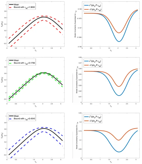
The results of model uncertainty guarantees for y|x0 with different ambiguity set Dlηl in (56) are shown in

Supplementary Figures S2 - S4. Note that forl =s0, e0, d0, the model uncertainty of ωl would affect both y1

andy4based on the ORR PGM, therefore we can see similar effects on both sides of volcano,y, in Supplementary

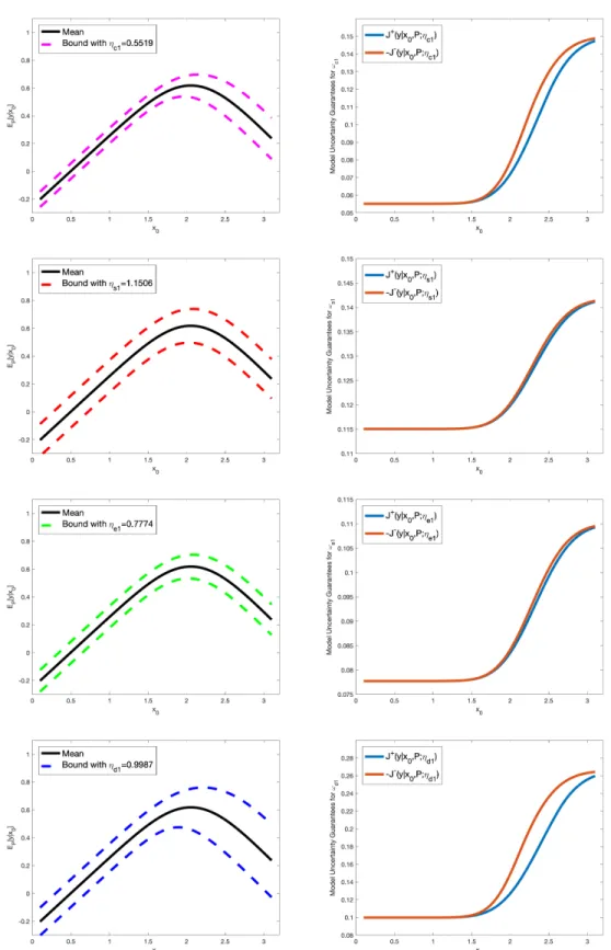
Figure S2. However, forl =c1, s1, e1, d1, the model uncertainty ofωlonly affects y1 based on the ORR PGM,

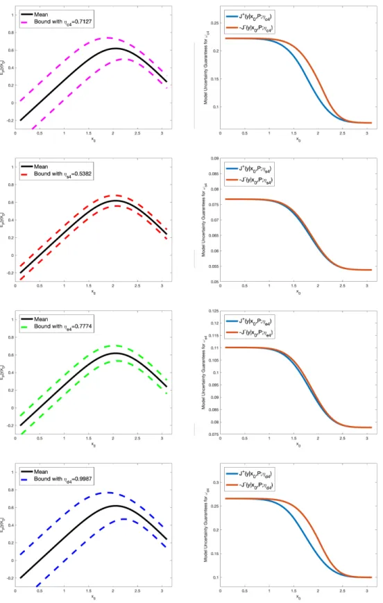
therefore it mainly affects the right side of the volcano,y, see Supplementary Figure S3. An analogous argument can be made for l=c4, s4, e4, d4 in Supplementary Figure S4.

Figure S2: Uncertainty bounds (dashed lines) for the QoIy (left column) and corresponding model uncertainty guarantees J_l±(y|x0, P;ηl) (right column), in equation (58), forωl, with model misspecification parameters ηl, l=s0, e0, d0, estimated from data (see Section 8 for details).

(19)

Figure S3: Uncertainty bounds (dashed lines) for the QoIy (left column) and corresponding model uncertainty guarantees J_l±(y|x0, P;ηl) (right column), in equation (58), forωl, with model misspecification parameters ηl, l=c1, s1, e1, d1, estimated from data.

(20)

Figure S4: Uncertainty bounds (dashed lines) for the QoIy (left column) and corresponding model uncertainty guarantees J_l±(y|x0, P;ηl) (right column), in equation (58), forωl, with model misspecification parameters ηl, l=c4, s4, e4, d4, estimated from data.

(21)

7

Uncertainty Quantification Bounds for QoIs

7.1

Attribution of QoI uncertainties in ORR PGM components

Based on the model uncertainty guarantees for each point on the volcano, y|x0, we can derive the UQ bounds

for the optimal reaction energy

y_maxQ = max x0 E Q[y|x0] (80) and optimal ∆GO xQ_max= argmax x0 EQ[y|x0] (81)

with different ambiguity sets, i.e.,Q∈ Dηl

l in (56), by max x0 y−(x0)≤ymaxQ ≤max_x 0 y+(x0) (82)

where y−(x0),y+(x0) are the lower and upper bounds of the model uncertainty guarantees atx0, and

min{x0|y+(x0)> ymax,−} ≤xmaxQ ≤max{x0|y+(x0)> ymax,−} (83)

whereymax,−= maxx0y−(x0), e.g., see Supplementary Figure S5 for the results with ambiguity setD

ηd4

d4 in (56)

where we focusing on the uncertainty of ωd4. Furthermore, we can also check the variability of xQmax by only

looking at the two worst cases and find the difference betweenxQ

maxof the lower bound and baseline mean, and

the difference between xQ

max of the upper bound and baseline mean. Moreover, we could compare the model

uncertainty of each component in the PGM by the area of uncertainty region, which is the area between the model uncertainty guarantees (dash lines in the figures above) within a given interval ([0,3]).

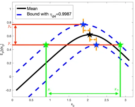
Figure S5: Uncertainty bounds for yQ

max (between red lines), xQmax (between green lines), andxQmax variability

(between orange lines) in the case where we only perturbing the model of ωd4 with model misspecification

parameterηd4, i.e. based on model uncertainty guaranteesJd±4(y|x0, P;ηc4) in equation (58) withQ∈ D

ηd4

d4 in

(56). And, the prediction of QoIs based on the nominal modelP, i.e., (xP

(22)

Table S5: UQ bounds foryQ

maxandxQmax, (yPmax= 0.6182,xPmax= 2.0537)

error type UQ bounds -yQ

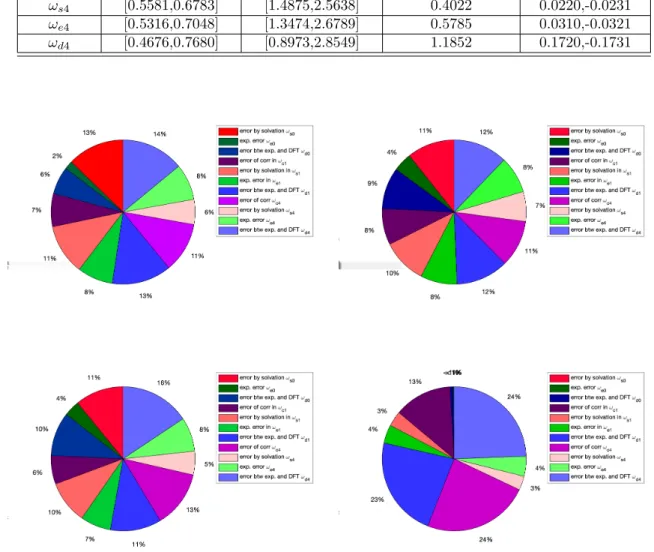
max UQ bounds -xQmax uncertainty region xQmax variability ωs0 [0.4815,0.7545] [1.1764,2.9009] 0.8246 -0.00005,-0.00005 ωe0 [0.5901,0.6301] [1.7125,2.3898] 0.2684 -0.0020,-0.0010 ωd0 [0.5190,0.6521] [1.2954,2.7999] 0.7463 -0.0101,-0.0010 ωc1 [0.5389,0.6974] [1.4795,2.7899] 0.4851 -0.0921,0.0910 ωs1 [0.4970,0.7395] [1.2554,2.8739] 0.7322 -0.0241,0.0240 ωe1 [0.5330,0.7035] [1.4144,2.7339] 0.5169 -0.0291,0.0290 ωd1 [0.4751,0.7605] [1.2404,3.1420] 0.8698 -0.1601,0.1590 ωc4 [0.4973,0.7384] [1.0463,2.7389] 0.9676 0.1680,-0.1691 ωs4 [0.5581,0.6783] [1.4875,2.5638] 0.4022 0.0220,-0.0231 ωe4 [0.5316,0.7048] [1.3474,2.6789] 0.5785 0.0310,-0.0321 ωd4 [0.4676,0.7680] [0.8973,2.8549] 1.1852 0.1720,-0.1731

Figure S6: Rankings for the model uncertainties of each errorsωlby the uncertainty bounds ofymaxQ (top left), xQ

max(top right), area of uncertainty region (bottom left), andxQmaxvariability (use the sum of the absolute values

in both worst cases) (bottom right), based on the model uncertainty guaranteesJ_l±(y|x0, P;ηl), in equation (58),

(23)

7.2

Attribution of QoI uncertainties to combined ORR PGM components

Here we evaluate the combined effects of each type of model uncertainty arising in each node of the ORR PGM, by correspondingly perturbing the nominal modelP, using Proposition 1:

I±(y|x0, P;η) =±inf c>0 h1 clog Z e±cf¯P(dx) +η c i (84)

where ¯f = y|x0−EP[y|x0], and the model misspecification parameter η equals to the combined model

mis-specification of each type estimated from data. We demonstrate such calculations in two separate examples next.

First, we consider the overall impact of the solvation, correlation, experimental and DFT errors. For instance, in the case of solvation all the corresponding error components in ORR PGM are independent, thus we have

η=ηs= n

X

i=0,1,4

EP{si}[R(Q(ωsi|Paωsi)||P(ωsi|Paωsi))] =ηs0+ηs1+ηs2 (85)

by (75). Working analogously with the remaining errors, we calculate (85) and the results are shown in the top of Supplementary Figure S7.

Second, we quantify the uncertainties of the energies corresponding tox,y1,y4, by considering their marginal

distributions and gathering the baseline model into two parts, i.e.

Py: y|x∼min(N(µy1(x), σ 2 y1(x)),N(µy4(x), σ 2 y4(x))) (86) where

µyi(x) =βyi,0+βyi,xx+βci,0+βsi,0+βei,0+βdi,0 (87)

σ2_y_i(x0) =σ2ci+σ 2 si+σ 2 ei+σ 2 di (88) fori= 1,4, and Px: x|x0∼ N(x0+βs0,0+βe0,0+βd0,0, σs20+σe20+σ2d0) (89)

then we can compute the model uncertainty guarantees,J±

x(f, P;ηx) andJyi±(f, P;ηyi) (similarly to (58)) with

model misspecification parametersηx=ηs0+ηe0+ηd0; on the other handηyi=ηci+ηsi+ηei+ηdi, similarly

(24)

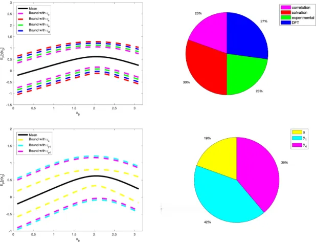
Figure S7: Top Left: Uncertainty bounds (dashed lines) for the QoI y based on the model uncertainty

I±(y|x0, P;ηl), in equation (84), of each types of errors (i.e. l = c:correlation, s:solvation, e:experiment, and

d:DFT) with corresponding combinedηl estimated from data; Top Right: Ranking foryQmaxandx Q

max

variabil-ity (results are the same) based on the model uncertainty I±(y|x0, P;ηl) of each types of errors. Bottom Left:

Uncertainty bounds (dashed lines) for the QoIy based on the model uncertainty guarantees J_l±(y|x0, P;ηl), in

equation (58), of each part (l =x, y1,y4) of PGM with corresponding combinedηl estimated from data;

Bot-tom Right: Ranking for the area of uncertainty region of each part based on the model uncertainty guarantees

J_l±(y|x0, P;ηl).

8

Estimating the Model Misspecification Parameters

η

,

η

l

Here we provide two perspectives on computing the model misspecification parameters η/ηl, the sencond one,

in (b), is applied for the results in the Main Text.

(a) Stress Tests for PGMs: First, the model misspecification parameters η, ηl > 0 in Proposition 1 and

Theorem 1 respectively are non-parametric perturbations of the entire modelP or each part of model,Pl. These η parameters are can be tuned “by hand” so that we can explore how the level of uncertainty will affect the QoI. In fact, comparing the model uncertainty ranking index (6) will give us a ranking of the impact of each component on the model on the QoIf. This is a form ofnon-parametric sensitivity analysisand is reminiscent in spirit of the stress tests used by financial institutions to protect against sudden changes and extreme uncertainty under various scenarios in some components of the model. This approach is especially useful in the case of very sparse or absent data for (parts of) the model, see examples in actuarial risk analysis, (130).

(b) Data-based estimation: In this case theη.ηlparameters are computed/estimated from data: we can also

consider the η as the “distance” between data and the PGMP, where data is represented by a histogram or a KDE approximation of the histogram, or any given particular model Qfrom data or expert knowledge. In this

(25)

case, we can estimateηl values constitutesurrogates for the distance of the baseline model from the unknown

“real” model. Clearly in this caseηl’s can be different for different components of the PGM. The methodologies

of determining the size of ambiguity set/model misspecification parameters are also investigated in operations research literature for distributionally robust optimization with many different viewpoints (126,131–136). Here we apply a data-based approach for the estimation of the ambiguity set, in the general spirit of the methodology in (130); however here our data-based approach is adaptated for PGMs, taking advantage of the graph structure and the KL chain rule on graphical models, (90).

Next, we present results on the data-based estimation of the model misspecification parameters. We focus on the ORR PGM, however the approach applies to any PGM built from data. Due to the chain rule of KL divergence, (28), here η:=R(Q||P) can be computed on a general PGM (Equation (2) of the Main Text) by the following decomposition η = Z logdQ dPdQ= n X i=1 EQ[R(Q(xi|PaXi)||P(xi|PaXi)]dxi = n X i=1 EQ h ηPaXi i i (90) where we denote by ηPaXi i = Z logq(xi|PaXi) p(xi|PaXi) q(xi|PaXi)dxi , (91)

conditioned on the parents PaXi. In our case where we consider primarily GBNs such as the ORR PGM, we

have p(Xi|PaXi) =p(Xi|X1:i−1) =N(βi0+β

T

i X1:i−1, σi2) for some βi0,βi, and σi2, i.e.,

Pi: Xi=βi0+βTi X1:i−1+i (92)

where i is a random variable with densitypi(x) =N(0, σ

2

i). We consider alternative models toP such as Qi: Xi=βi0+βTi X1:i−1+ ˜i (93)

where ˜i follows another approximate distribution of the data with densityq˜i(x), for instance any histogram or

KDE such as the one shown on Supplementary Figure S8. Therefore, for given PaXi =X1:i−1, we have

thus, we have thatηPaXi

i is independent of PaXi; in fact, we have

η_iPaXi ≡ηi=

Z

logq˜i(x)

pi(x)

q˜i(x)dx , (95)

in both Equations 6 and 10 of the Main Text and methods .

Next, we demonstrate the estimation of model misspecification based on (95). Here we refer to the random variablesc4for the PGM in Figure 2(b) in the Main Text, and show corresponding available data in a histogram

with bin width 0.05 in Supplementary Figure S8. Then for the Gaussian model Pωc4 obtained by fitting data

with Maximum-Likelihood-Estimation in Section 4, we computeηc4 by consideringQω˜c4 as the histogram, i.e.,

q_ωhist_˜ c4(x) = m X k=1 νk nhI(x∈Bk), (96)

(26)

whereB1, . . . , Bmare the histogram bins,his the bin width,nis the number of observations andνkis the number

of observations inBk. Then by (90) we haveηc4= 0.7127. Moreover, we can also consider an alternative model

Qω˜c4 given by a kernel density estimator (KDE) considered here as a high resolution but smooth approximation

of the histogram, namely

qKDE_˜_ω_c₄ (x) = n X k=1 1 nhK( x−xi h ), (97)

where K(·) is the normal kernel smoothing function with bin width 0.05, (x1, . . . , xn) are the samples of ωc4,

and then with the same steps, we get ηc4 = 0.1285, see Supplementary Figure S8. Similarly, we can consider

other KDE kernels, (137), or any other probabilistic representations of the data in the histogram. It can be shown using the weak continuity properties of the KL divergence, (118), that R(Qω˜c4||Pωc4) will converge to

R(Qωc4||Pωc4) in the large data limit, where Qωc4 is the real distribution of ωc4. For more general results and

a broad discussion of the vast literature on divergence estimation we also refer to results in (138–141) and references therein.

Figure S8: Different probabilistic models for ωc4, see also Figure 2(b) in Main Text. We can represent the data

of ωc4 by histogram, i.e., considering the histogram Qhistω˜c4 with bin width 0.05 corresponded to the available

data; Pωc4 is the Gaussian model fitted to the data; then we can compute ηc4 by (95) and obtain ηc4= 0.7127.

Alternatively, we can consider a modelQKDE

˜

ωc4 built by KDE with a normal kernel and bin width 0.05 from the

(27)

REFERENCES AND NOTES

1. A. Hospital, J. R. Goñi, M. Orozco, J. L. Gelpí, Molecular dynamics simulations: Advances and

applications.

Adv. Appl. Bioinforma. Chem.

8

, 37–47 (2015).

2. J. Sehested, K. E. Larsen, A. L. Kustov, A. M. Frey, T. Johannessen, T. Bligaard, M. P. Andersson, J.

K. Nørskov, C. H. Christensen, Discovery of technical methanation catalysts based on computational

screening.

Top. Catal.

45

, 9–13 (2007).

3. D. A. Hansgen, D. G. Vlachos, J. G. Chen, Using first principles to predict bimetallic catalysts for the

ammonia decomposition reaction.

Nat. Chem.

2

, 484–489 (2010).

4. J. A. Pople, Nobel lecture: Quantum chemical models.

Rev. Mod. Phys.

71

, 1267–1274 (1999).

5. S. Skogestad, I. Postlethwaite,

Multivariable Feedback Control: Analysis and Design

(Wiley New

York, 2007), vol. 2.

6. F. Abild-Pedersen, J. Greeley, F. Studt, J. Rossmeisl, T. R. Munter, P. G. Moses, E. Skúlason, T.

Bligaard, J. K. Nørskov, Scaling properties of adsorption energies for hydrogen-containing

molecules on transition-metal surfaces.

Phys. Rev. Lett.

99

, 016105 (2007).

7. F. Calle-Vallejo, J. Tymoczko, V. Colic, Q. H. Vu, M. D. Pohl, K. Morgenstern, D. Loffreda, P.

Sautet, W. Schuhmann, A. S. Bandarenka, Finding optimal surface sites on heterogeneous catalysts

by counting nearest neighbors.

Science

350

, 185–189 (2015).

8. J. L. Lansford, A. V. Mironenko, D. G. Vlachos, Scaling relationships and theory for vibrational

frequencies of adsorbates on transition metal surfaces.

Nat. Commun.

8

, 1842 (2017).

9. M. Salciccioli, M. Stamatakis, S. Caratzoulas, D. G. Vlachos, A review of multiscale modeling of

metal-catalyzed reactions: Mechanism development for complexity and emergent behavior.

Chem.

Eng. Sci.

66

, 4319–4355 (2011).

10. A. Saltelli, M. Ratto, S. Tarantola, F. Campolongo, Sensitivity analysis for chemical models.

Chem.

Rev.

105

, 2811–2828 (2005).

(28)

11. H. Rabitz, M. Kramer, D. Dacol, Sensitivity analysis in chemical kinetics.

Annu. Rev. Phys. Chem.

34

, 419–461 (1983).

12. J. E. Sutton, W. Guo, M. A. Katsoulakis, D. G. Vlachos, Effects of correlated parameters and

uncertainty in electronic-structure-based chemical kinetic modelling.

Nat. Chem.

8

, 331–337 (2016).

13. J. Feng, J. Lansford, A. Mironenko, D. B. Pourkargar, D. G. Vlachos, M. A. Katsoulakis,

Non-parametric correlative uncertainty quantification and sensitivity analysis: Application to a Langmuir

bimolecular adsorption model.

AIP Adv.

8

, 035021 (2018).

14. S. Gautier, S. N. Steinmann, C. Michel, P. Fleurat-Lessard, P. Sautet, Molecular adsorption at

Pt(111). How accurate are DFT functionals?

Phys. Chem. Chem. Phys.

17

, 28921–28930 (2015).

15. J. Wellendorff, K. T. Lundgaard, A. Møgelhøj, V. Petzold, D. D. Landis, J. K. Nørskov, T. Bligaard,

K. W. Jacobsen, Density functionals for surface science: Exchange-correlation model development

with Bayesian error estimation.

Phys. Rev. B

85

, 235149 (2012).

16. J. Wellendorff, T. L. Silbaugh, D. Garcia-Pintos, J. K. Nørskov, T. Bligaard, F. Studt, C. T.

Campbell, A benchmark database for adsorption bond energies to transition metal surfaces and

comparison to selected DFT functionals.

Surf. Sci.

640

, 36–44 (2015).

17. C. C. Aggarwal, in

Managing and Mining Uncertain Data

, C. C. Aggarwal, Ed. (Springer US,

Boston, MA, 2009), pp. 1–36.

18. J. A. Vrugt, C. J. F. ter Braak, M. P. Clark, J. M. Hyman, B. A. Robinson, Treatment of input

uncertainty in hydrologic modeling: Doing hydrology backward with Markov chain Monte Carlo

simulation.

Water Resour. Res.

44

, W00B09 (2008).

19. J. Freer, K. Beven, B. Ambroise, Bayesian estimation of uncertainty in runoff prediction and the

value of data: An application of the GLUE approach.

Water Resour. Res.

32

, 2161–2173 (1996).

20. N. Friedman, M. Linial, I. Nachman, D. Pe'er, Using Bayesian networks to analyze expression data.

(29)

21. I. M. Sobol, Global sensitivity indices for nonlinear mathematical models and their Monte Carlo

estimates.

Math. Comput. Simul.

55

, 271–280 (2001).

22. A. Saltelli, P. Annoni, I. Azzini, F. Campolongo, M. Ratto, S. Tarantola, Variance based sensitivity

analysis of model output. Design and estimator for the total sensitivity index.

Comput. Phys.

Commun.

181

, 259–270 (2010).

23. L. Landau, E. Lifshitz, in

Perspectives in Theoretical Physics

, L. P. Pitaevski, Ed. (Pergamon,

1992), pp. 287–297.

24. S. Taverniers, F. J. Alexander, D. M. Tartakovsky, Noise propagation in hybrid models of nonlinear

systems: The Ginzburg–Landau equation.

J. Comput. Phys.

262

, 313–324 (2014).

25. D. Koller, N. Friedman,

Probabilistic Graphical Models: Principles and Techniques

(MIT press,

2009).

26. Z. Ghahramani, Probabilistic machine learning and artificial intelligence.

Nature

521

, 452–459

(2015).

27. P. Dupuis, M. A. Katsoulakis, Y. Pantazis, P. Plechác, Path-space information bounds for

uncertainty quantification and sensitivity analysis of stochastic dynamics.

SIAM-ASA J. Uncertain.

4

, 80–111 (2016).

28. M. A. Katsoulakis, L. Rey-Bellet, J. Wang, Scalable information inequalities for uncertainty

quantification.

J. Comput. Phys.

336

, 513–545 (2017).

29. J. E. Sutton, D. G. Vlachos, Effect of errors in linear scaling relations and Brønsted–Evans–Polanyi

relations on activity and selectivity maps.

J. Catal.

338

, 273–283 (2016).

30. S. Deshpande, J. R. Kitchin, V. Viswanathan, Quantifying uncertainty in activity volcano

relationships for oxygen reduction reaction.

ACS Catal.

6

, 5251–5259 (2016).

(30)

31. D. R. Palo, J. D. Holladay, R. T. Rozmiarek, C. E. Guzman-Leong, Y. Wang, J. Hu, Y.-H. Chin, R.

A. Dagle, E. G. Baker, Development of a soldier-portable fuel cell power system: Part I: A

bread-board methanol fuel processor.

J. Power Sources

108

, 28–34 (2002).

32. H. A. Gasteiger, N. M. Marković, Just a dream—Or future reality?

Science

324

, 48–49 (2009).

33. W. Sheng, H. A. Gasteiger, Y. Shao-Horn, Hydrogen oxidation and evolution reaction kinetics on

platinum: Acid vs alkaline electrolytes.

J. Electrochem. Soc.

157

, B1529 (2010).

34. J. Durst, A. Siebel, C. Simon, F. Hasché, J. Herranz, H. A. Gasteiger, New insights into the

electrochemical hydrogen oxidation and evolution reaction mechanism.

Energy Environ. Sci.

7

,

2255–2260 (2014).

35. N.-T. Suen, S.-F. Hung, Q. Quan, N. Zhang, Y.-J. Xu, H. M. Chen, Electrocatalysis for the oxygen

evolution reaction: Recent development and future perspectives.

Chem. Soc. Rev.

46

, 337–365

(2017).

36. O. Antoine, Y. Bultel, R. Durand, Oxygen reduction reaction kinetics and mechanism on platinum

nanoparticles inside Nafion®.

J. Electroanal. Chem.

499

, 85–94 (2001).

37. A. Holewinski, S. Linic, Elementary mechanisms in electrocatalysis: Revisiting the ORR tafel slope.

J. Electrochem. Soc.

159

, H864–H870 (2012).

38. M. Núñez, J. L. Lansford, D. G. Vlachos, Optimization of the facet structure of transition-metal

catalysts applied to the oxygen reduction reaction.

Nat. Chem.

11

, 449–456 (2019).

39. D. M. Chickering, in

Learning from Data: Artificial Intelligence and Statistics V

, D. Fisher, H.-J.

Lenz, Eds. (Springer New York, 1996), pp. 121–130.

40. G. F. Cooper, The computational complexity of probabilistic inference using bayesian belief

networks.

Artif. Intell.

42

, 393–405 (1990).

(31)

42. T. Hofmann, B. Schölkopf, A. J. Smola, Kernel methods in machine learning.

Ann. Stat.

36

, 1171–

1220 (2008).

43. K. Um, E. J. Hall, M. A. Katsoulakis, D. M. Tartakovsky, Causality and Bayesian Network PDEs for

multiscale representations of porous media.

J. Comput. Phys.

394

, 658–678 (2019).

44. G. Kresse, J. Furthmüller, Efficient iterative schemes forab initiototal-energy calculations using a

plane-wave basis set.

Phys. Rev. B

54

, 11169–11186 (1996).

45. B. Hammer, L. B. Hansen, J. K. Norskov, Improved adsorption energetics within density-functional

theory using revised Perdew-Burke-Ernzerhof functionals.

Phys. Rev. B

59

, 7413–7421 (1999).

46. S. Grimme, J. Antony, S. Ehrlich, H. Krieg, A consistent and accurate ab initio parametrization of

density functional dispersion correction (DFT-D) for the 94 elements H-Pu.

J. Chem. Phys.

132

,

154104 (2010).

47. H. J. Monkhorst, J. D. Pack, Special points for Brillouin-zone integrations.

Phys. Rev. B

13

, 5188–

5192 (1976).

48. F. D. Murnaghan, The compressibility of media under extreme pressures.

Proc. Natl. Acad. Sci.

U.S.A.

30

, 244–247 (1944).

49. S. R. Bahn, K. W. Jacobsen, An object-oriented scripting interface to a legacy electronic structure

code.

Comput. Sci. Eng.

4

, 56–66 (2002).

50. S. Meng, E. G. Wang, S. Gao, Water adsorption on metal surfaces: A general picture from density

functional theory studies.

Phys. Rev. B

69

, 195404 (2004).

51. J. P. Perdew, K. Burke, M. Ernzerhof, Generalized gradient approximation made simple.

Phys. Rev.

Lett.

77

, 3865–3868 (1996).

52. L. P. Granda-Marulanda, S. Builes, M. T. M. Koper, F. Calle-Vallejo, Influence of Van der Waals

interactions on the solvation energies of adsorbates at Pt-based electrocatalysts.

ChemPhysChem

20

,

2968–2972 (2019).

(32)

53. D. A. McQuarrie,

Statistical Mechanics

(University Science Books, 2000).

54. K. Gourgoulias, M. A. Katsoulakis, L. Rey-Bellet, J. Wang, How biased is your model?

Concentration inequalities, information and model bias.

IEEE Trans. Inf. Theory

, 1–1 (2020).

55. S. Choi, C. J. Kucharczyk, Y. Liang, X. Zhang, I. Takeuchi, H.-I. Ji, S. M. Haile, Exceptional power

density and stability at intermediate temperatures in protonic ceramic fuel cells.

Nat. Energy

3

, 202–

210 (2018).

56. C. K. Dyer, Fuel cells for portable applications.

J. Power Sources

106

, 31–34 (2002).

57. G. Sievi, D. Geburtig, T. Skeledzic, A. Bösmann, P. Preuster, O. Brummel, F. Waidhas, M. A.

Montero, P. Khanipour, I. Katsounaros, J. Libuda, K. J. J. Mayrhofer, P. Wasserscheid, Towards an

efficient liquid organic hydrogen carrier fuel cell concept.

Energy Environ. Sci.

12

, 2305–2314