Combinatorial approach using wavelet analysis and artificial neural network for short-term load forecasting

(1)

University of Wollongong

Research Online

Faculty of Engineering and Information

Sciences - Papers: Part A

Faculty of Engineering and Information

Sciences

1-1-2014

Combinatorial approach using wavelet analysis and artificial neural network

for short-term load forecasting

Dao Hoang Vu

University of Wollongong, [email protected]

Kashem M. Muttaqi

Ashish P. Agalgaonkar

Follow this and additional works at: https://ro.uow.edu.au/eispapers

Part of the Engineering Commons, and the Science and Technology Studies Commons

Recommended Citation

Vu, Dao Hoang; Muttaqi, Kashem M.; and Agalgaonkar, Ashish P., "Combinatorial approach using wavelet analysis and artificial neural network for short-term load forecasting" (2014). Faculty of Engineering and Information Sciences - Papers: Part A. 3883.

https://ro.uow.edu.au/eispapers/3883

Research Online is the open access institutional repository for the University of Wollongong. For further information contact the UOW Library: [email protected]

(2)

Combinatorial approach using wavelet analysis and artificial neural network for

short-term load forecasting

Abstract

Short term load forecasting is critically important in modern electricity networks since it helps provide supportive information for reliable power system operation in competitive electricity market environment. In this paper, the wavelet analysis based neural network model is employed to forecast the electricity demand in short-term period. The wavelet analysis helps to decompose the electricity demand data into different frequency bands. The Fourier transform is then employed to reveal the significant lags of these decomposed components. These lags are then used as inputs of neural network model to forecast the future values of each decomposed component. Finally, the forecasted components are combined together to form the electricity demand forecast. A case study has been reported in the paper by acquiring the data for the state of New South Wales, Australia. MAPE is used to validate the proposed model and the results show that the proposed method is promising for short term load forecasting.

Keywords

artificial, term, network, neural, wavelet, short, forecasting, combinatorial, load, approach, analysis

Disciplines

Engineering | Science and Technology Studies

Publication Details

D. Vu, K. M. Muttaqi & A. P. Agalgaonkar, "Combinatorial approach using wavelet analysis and artificial neural network for short-term load forecasting," in 2014 Australasian Universities Power Engineering Conference (AUPEC 2014), 2014, pp. 1-6.

(3)

Combinatorial Approach using Wavelet Analysis

and Artificial Neural Network for Short-term Load

Forecasting

D. H. Vu,

Student member, IEEE

, K. M. Muttaqi,

Senior Member, IEEE

, A. P. Agalgaonkar,

Senior Member, IEEE

Australian Power Quality and Reliability Center, School of Electrical Computer and Telecommunications Engineering

University of Wollongong, Wollongong, NSW, Australia [email protected]; [email protected]; [email protected]

Abstract — Short term load forecasting is critically important in modern electricity network since it helps provide supportive information in reliable power system operation and competitive electricity market. In this paper, the wavelet analysis based neural network model is employed to forecast the electricity demand in short-term period. The wavelet analysis helps to decompose the electricity demand data into different frequency bands. The Fourier transform is then employed to reveal the significant lags of these decomposed components. These lags are then used as inputs of neural network model to forecast the future values of each decomposed component. Finally, the forecasted components are combined together to form the electricity demand forecast. A case study has been reported in this paper by acquiring the data from the state of New South Wales, Australia. MAPE is used to validate the proposed model and the result shows that the proposed method is promising in forecasting the load in short term period.

Index Terms—Neural Network; Electricity Demand Forecasting;

Wavelet Analysis; Fourier Transform; Weather Variables.

I. INTRODUCTION

Load forecasting is critically important in operation of electricity system since it can provide supportive information to help the system work securely. Moreover, good results in load forecasting can help significantly improve the economic factors of the power network operation [1]. Specifically, short term load forecasting, which deals with the time scale from few minutes up to few weeks ahead [2] is crucial since it may affect directly the balance between load and generation.

With the importance of forecasting role in operating the power system, a very wide range of forecasting techniques were employed to build the forecasting model in short-term period [2]. The regression model is often used in forecasting since it can reveal the relationship between demand and other external variables such as weather variables [3]. The Box-Jenkins model has the advantage in linking the forecasted demand to the demand in historical data [4], [5]. While these methods employ the linear technique to forecast the demand, the neural network is popularly used in tracing the nonlinear properties of the load variation [6]. The other techniques such

as application of Kalman Filter [7] and support vector machine [8], [9] also help improve the forecasting results.

The hybrid model is often employed in load forecasting since the cooperation of the different techniques may result in good forecasts. The combination of wavelet and neural network can convey a very good model in forecasting load demand [10], [11]. The wavelet technique is well known for its ability to decompose the time series signal into different frequency bands [12]. Each of these decomposed components carries some specific details of the original signal in the chosen frequency band. More importantly, these components can be composed again to derive the original signal. The neural network is widely used in load forecasting since it can extract the nonlinear relationship between demand and the input variables [13]. In [14], it is illustrated that the decomposed components from wavelet analysis of demand data can be successfully used as inputs for the neural network forecasting model. In this paper, the wavelet is used to decompose both demand data and temperature data into low frequency and high frequency components. The Fourier transform is then used to reveal the demand patterns in frequency domain. These patterns provide the critical information to select the lags in demand and temperature components as inputs for the neural network model. In the next step, the neural network will be used to forecast the components separately. Finally, the future demand values are determined from these forecasted components.

The paper is organised as follows: Section II highlights the pattern of the electricity demand. In section III, the wavelet and neural network are introduced for load forecasting. Section IV presents some results and discussion. Section V gives some concluding remarks.

II. ELECTRICITY DEMAND PATTERNS

Electricity demand is influenced by many factors which cause the electricity to be combination of some periodic and noise signals. In general, specific activities or habits of people in each of the periodic intervals such as daily, weekly, seasonally, require different consumption of electricity. This leads to the inclusion of periodic signal in the electricity demand. The noise components often come with random

This work is supported by Hong Duc, Thanh Hoa – UOW research scholarship program.

(4)

2 electricity activity during a day or even a minute. It relates to

the variation of critical decision of using electricity equipment. Revealing the patterns of electricity demand is enormously important since it can help expand understanding about the detail of changes in different components included in the demand data, and provide the significant information contributing to the forecasting model.

A. Time Series Pattern

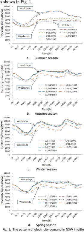
The predominant pattern of electricity demand in Denmark is reported to be different for working days and non-working days [15]. In this subsection, the time series data is presented to reveal the pattern of electricity demand for the state of NSW, Australia for the typical daily and weekly seasonal patterns as shown in Fig. 1.

a. Summer season

b. Autumn season

c. Winter season

d. Spring season

Fig. 1. The pattern of electricity demand in NSW in different seasons

It can be seen from Fig. 1 that there are two distinctive patterns of load demand which are working days (from Monday to Friday) and non-working days (Saturday, Sunday, and holiday). The demand in the working day is greater than that in the non-working day. In the working days, the demand pattern is very strong, which can lead to nearly repetition of demand curve in the following day. In the non-working days, the demand on Sunday is generally lower than that on Saturday, but higher than that of a public holiday. Furthermore, the variation of load in one day is strongly affected by seasons such as Summer, Autumn, Winter and Spring.

Based on the time series pattern as in Fig. 1, the potential inputs for the forecasting model may include the lags of one day, one week, and season factors. The significance of each lag is however not clear in this time series representation since the significant level of the lag is not illustrated in those time series depictions.

B. Fourier Transform of Electricity Demand

Fourier transform will provide more supportive information to understand the pattern in the electricity demand [16]. By applying the Fourier transform, the obtained representation will depict the repetition of the signal in different bands of frequency. If the frequency to appear of signal in a specific band is high, meaning that there are more repetition of that signal in whole time period, and the lag corresponding to that frequency band is more significant to be used to forecast the future values.

The electricity demand data of every 30 minutes from state of NSW, Australia in year 1999 is used for illustration and the spectrum is shown as in Fig. 2.

Fig. 2.Fourier transform of electricity demand in NSW

It can be seen from Fig. 2 that the most dominant frequencies are associated with seasonally, weekly, daily, and a half of daily varying data. The lags corresponding to these frequency bands are considered significant, and they can be selected to be included to the forecasting model.

In forecasting electricity demand, the noise attaching to the fundamental components may affect the significance of the chosen inputs. Moreover, this noise can cause distortion in the forecasting result if the inputs are not carefully de-noised.

(5)

3

III. WAVELET NEURAL NETWORK FOR LOAD FORECASTING Wavelet neural network is the combination between the wavelet analysis and neural network model, which can be successfully used in forecasting the future electricity demand. The wavelet is well known with the ability to decompose the series signal into different frequency bands [12]. The decomposed components may provide more supportive information to the neural network model, which is used to forecast the electricity demand.

A. Wavelet Analysis

Wavelet analysis can help decompose the historical electricity demand into different components belonging to different bands of frequency based on a mother wavelet function. The process of typical 3-level wavelet decomposition is shown in Fig. 3. The original signal S(t) is put through high pass and low pass filters, and the outputs are the detail component at level 1 (D1) and approximation at level 1 (A1). A1 is then put in the filters at level 2 to get the detail and approximation at second level D2 and A2 respectively. The third analysis level is applied to A2 to derive the detail and approximation at this level D3 and A3.

Fig. 3.A typical 3-level wavelet decomposition diagram

The details (D1, D2, and D3) and approximation (A3) components in Fig. 3 are orthogonal, and they are expected to give more contributively independent information to the neural network forecasting model.

B. Neural Network

Neural network is widely employed in load forecasting since it can disclose the non-linear relationship between demand and other variables [17]. The neural network used in this paper is a feed-forward neural network which composes of an input layer, one or more hidden layers, and an output layer [18]. The typical diagram of a neural network is given in Fig. 4.

Fig. 4. Architecture of a neural network

As shown in Fig. 4, the n inputs x1,x2,...x_n and a bias

constant from the input layer are fed to the hidden layer with m

neurons N1,N2,...N_m via a weight matrix wjk. The outputs of

the hidden layer are used as inputs for the output layer which contains only one neuronN_o. The information from output layer is then employed to forecast the associated values. In each neuron N1,N2,...N_mandNo, there are two processes: (1) the inputs are summed by the summation function S, and (2) this summation is put through an activation function f to produce the output.

C. Forecasting Model

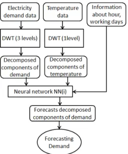
With the application of the wavelet technique and neural network model, the forecasting process is proposed as in Fig. 5. The electricity demand and temperature are decomposed using wavelet analysis. All decomposed components in conjunction with the hourly and daily information will be used as inputs for the neural networks to forecast the decomposed components of electricity demand for e.g. A3, D3, D2, and D1. The selection of lags for the inputs in this step is critical and the Fourier transform (as described in subsection II-B) helps in designing the process. Finally, the combination of forecasting results of the decomposed components will be employed to provide the forecasting of electricity demand.

Fig. 5. Conceptual diagram

D. Validation Technique

To validate the forecasting results, some methods such as Mean Absolute Error (MAE), Mean Average Percentage Error (MAPE) can be used. In this paper, MAPE is used for the validating purpose. The formula of MAPE is given as in (1).

% 100 * 1 1

∑

= − = n t t t t A M A n MAPE (1)

Where A_tand M_tare actual demand and modelled demand at time t respectively, and n is the number of forecasting points.

(6)

4

IV. RESULTS AND DISCUSSION

A case study has been reported with the assistance of historical data collected from the state of NSW, Australia for the years 1999 to 2000. The electricity demand data including all sectors, were collected from Australian energy market operator (AEMO) [19]. The temperature obtained at Sydney airport station [20] are assumed to represent the entire state of NSW since around 75% of population of NSW are in Sydney and the surrounding areas. Matlab and Microsoft-excel are employed to implement the requisite calculations. The data in year 1999 is used to train the proposed forecasting model. This model is then tested on the data in year 2000. The results for two typical extreme seasons which are winter and summer, and entire period are presented.

A. Wavelet Analysis

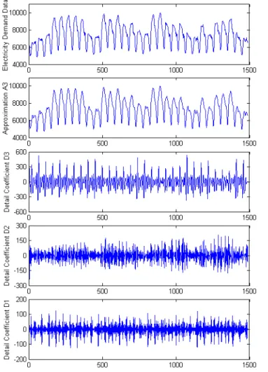
There are many types of mother wavelet which can be used to decompose a signal [21]. In all the mother wavelets, the Daubechies wavelet of order 4 (Db4) is found to be tremendously effective in decomposing the electricity demand data [22]. In this paper, Db4 is employed in electricity demand analysis. The typical electricity demand data at the beginning of the year 1999 is put in wavelet analysis and the results are given as in Fig. 6.

Fig. 6. Wavelet decomposition components

It can be seen from Fig. 6 that the approximation A3 has the form quite similar to the original data. The magnitude of A3 is nearly equal to the magnitude of the original signal. This

is the most important signal to recover the original signal, and it is expected to give the most important information in forecasting the electricity demand. For the detail coefficients, the magnitude of the coefficient decreases when the level of it decreases (from D3 to D1). This denotes that the lower the level of detailed coefficient, the less the influence on the original signal of that coefficient. In addition, the frequency of change in the coefficient increases vastly from D3 to D1. For D1, it can be seen that the frequency of the signal is high, like a noise, and this noise is expected to provide least useful information to the forecasting model.

B. Forecasting of the Frequency Components

Choosing the lags to forecast the decomposed components is exceedingly important since it affect the forecasting results. The authors in [14] used same size of lags for forecasting the detail components D2 and D3, and then shorter length of lags in forecasting the approximation component A3. That opinion does not guarantee that the chosen lags are the best selection of lag components.

In the proposed study, the decomposed components in sub section IV-A will be converted to the frequency domain using Fourier transform to reveal the significant lags, which have high potential to be included in the forecasting model. Fig. 7 gives more details about the Fourier transform of the components in Fig. 6.

(7)

5

It can be seen from Fig. 7 that each signal has a separate dominant frequency of repetition because they are the output of the wavelet analysis. Take the approximation A3 for example, it has the dominant repetition at 1week, 1 day, a half of day, and a quarter of day. In addition, the lag value of 30 minutes brings the most updated information to the current value. All the lags of repetition and 30 minutes lags are considered as significant variables and they can be used in the forecasting model. Set each step to be 30 minutes, and then convert the lags in time scale of 1week, 1 day, a half of day, and a quarter of day and 30 minutes into the steps, so the lags become 366, 48, 24, 12, 1 steps respectively. Those lags will be input to the forecasting model to forecast future value of A3. A similar selection of lag steps is applied to the other components, and the details are given in Table I.

TABLE I. LAG SELECTION FOR NEURAL NETWORK INPUTS NN(i) Decomposed component Lag steps

1 Approximation A3 366, 48, 24, 12, 1 2 Detail coefficient D3 16,12,1 3 Detail coefficient D2 8,6,1 4 Detail coefficient D1 1

It can be seen from Table I that the number of the significant lag steps reduces from A3 to D1. This illustrates that more significant signal may need more lags to represent. In addition, for the low frequency component, the lags often come with longer steps. For the very high frequency component D1, the variation is more random, so referring to more lags does not help to improve the forecasts. Consequently, only one step lag is selected in forecasting this component. The lag steps in Table I also recommend that if we wish to forecast one day or longer periods ahead, all the useful information for the forecast will come from A3 with the lag being greater or equal to 48 steps.

After determining the significant lags, neural network which is described in subsection III. B. will be used to forecast each decomposed component. For this study, nonlinear sigmoid function and linear function are chosen as activation function for the neurons in hidden layer and output layer, respectively. Mean absolute error (MAE) is selected as the performance metric of the network. The back propagation algorithm is used to train the network, and Levenburg-Marquardt method is applied as the optimization manner. The number of neurons in the hidden layer is chosen to be 20,

which is based on the practical work experience.

C. Load Forecasting

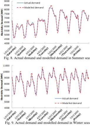
From the component forecasts in subsection IV.B, the load forecasting is derived by making the summation of the forecasted components together. The typical results representing for the typical seasons which are summer and winter in NSW is given in Fig. 8 and 9.

Fig. 8. Actual demand and modelled demand in Summer season

Fig. 9. Actual demand and modelled demand in Winter season

From the Fig. 8 and Fig. 9, it can be seen that the correspondence between the actual demand and forecasted demand is very close. The value of demand on Tuesday (4/1/2000) is however slightly over-forecasted because the temperature on that day increased abruptly as shown in Fig. 10. With the increase of temperature, both the actual and modelled demand show increment, and the modelled demand is a bit more sensitive to the change of temperature. This leads to the over forecasted value in this circumstance.

Fig. 10. Variation of temperature in typical Summer week

For validation purpose, the MAPE value of the typical summer, winter and for whole period is estimated as in Table II.

TABLE II. MAPEVALUES OF FORECASTING RESULTS Time period MAPE values

Typical Winter week 1.28 Typical Summer week 1.61 Whole year 2000 1.31

The MAPE values in Table II show that the model accurately mimics the real data in the winter season as

(8)

6

compared to the summer season. This is due to the dependence of demand on temperature in the winter season is stronger than that in the summer season in the state of New South Wales, Australia. In overall, the MAPE values are quite low, indicating the effectiveness of the proposed forecasting model.

V. CONCLUSION

In this paper, the neural network in conjunction with wavelet analysis is used to forecast the electricity demand in short-term period. The demand pattern can be revealed by employing the time series and Fourier transform analysis where the latter technique can depict more information about the significant lags. The wavelet analysis helps to decompose the demand data into various components which are located in different frequency bands. The Fourier transform is then applied to reveal the pattern of the decomposed components and the significant lags are determined. These significant lags are then used to form the inputs for the neural network model which is employed to forecast the corresponding components. Finally, the forecasted components are combined to derive the forecasted electricity demand. The calculated MAPE values associated with identifying the goodness of forecasting results indicate the robustness of the proposed model.

REFERENCES

[1] D. K. Ranaweera, G. G. Karady, and R. G. Farmer, "Economic impact analysis of load forecasting," Power Systems, IEEE Transactions on, vol. 12, pp. 1388-1392, 1997.

[2] M. A. Abu-El-Magd and N. K. Sinha, "Short-Term Load Demand Modeling and Forecasting: A Review," Systems, Man and Cybernetics, IEEE Transactions on, vol. 12, pp. 370-382, 1982. [3] M. O. Oliveira, D. P. Marzec, G. Bordin, A. S. Bretas, and D.

Bernardon, "Climate change effect on very short-term electric load forecasting," in PowerTech, 2011 IEEE Trondheim, 2011, pp. 1-7. [4] S. S. Pappas, L. Ekonomou, P. Karampelas, D. C. Karamousantas,

S. K. Katsikas, G. E. Chatzarakis, and P. D. Skafidas, "Electricity demand load forecasting of the Hellenic power system using an ARMA model," Electric Power Systems Research, vol. 80, pp. 256-264, 2010.

[5] S. S. Pappas, L. Ekonomou, D. C. Karamousantas, G. E. Chatzarakis, S. K. Katsikas, and P. Liatsis, "Electricity demand loads modeling using AutoRegressive Moving Average (ARMA) models," Energy, vol. 33, pp. 1353-1360, 2008.

[6] R. S. Elias, F. Liping, and M. I. M. Wahab, "Electricity load forecasting based on weather variables and seasonalities: A neural

network approach," in Service Systems and Service Management (ICSSSM), 2011 8th International Conference on, 2011, pp. 1-6. [7] R. Shankar, K. Chatterjee, and T. K. Chatterjee, "A very short-term

load forecasting using Kalman filter for load frequency control with economic load dispatch," Journal of Engineering Science and Technology Review, 2012.

[8] E. Ceperic, V. Ceperic, and A. Baric, "A Strategy for Short-Term Load Forecasting by Support Vector Regression Machines," Power Systems, IEEE Transactions on, vol. 28, pp. 4356-4364, 2013. [9] A. Setiawan, I. Koprinska, and V. G. Agelidis, "Very short-term

electricity load demand forecasting using support vector regression," in Neural Networks, 2009. IJCNN 2009. International Joint Conference on, 2009, pp. 2888-2894.

[10] G.-C. Liao, "Hybrid Improved Differential Evolution and Wavelet Neural Network with load forecasting problem of air conditioning," International Journal of Electrical Power & Energy Systems, vol. 61, pp. 673-682, 2014.

[11] A. Deihimi, O. Orang, and H. Showkati, "Short-term electric load and temperature forecasting using wavelet echo state networks with neural reconstruction," Energy, vol. 57, pp. 382-401, 2013. [12] S. G. Mallat, "A theory for multiresolution signal decomposition:

the wavelet representation," Pattern Analysis and Machine Intelligence, IEEE Transactions on, vol. 11, pp. 674-693, 1989. [13] J. W. Taylor and R. Buizza, "Neural network load forecasting with

weather ensemble predictions," Power Systems, IEEE Transactions on, vol. 17, pp. 626-632, 2002.

[14] A. R. Reis and A. P. Alves da Silva, "Feature extraction via multiresolution analysis for short-term load forecasting," Power Systems, IEEE Transactions on, vol. 20, pp. 189-198, 2005. [15] F. M. Andersen, H. V. Larsen, and R. B. Gaardestrup, "Long term

forecasting of hourly electricity consumption in local areas in Denmark," Applied Energy, vol. 110, pp. 147-162, 2013.

[16] G. Che, P. B. Luh, L. D. Michel, W. Yuting, and P. B. Friedland, "Very Short-Term Load Forecasting: Wavelet Neural Networks With Data Pre-Filtering," Power Systems, IEEE Transactions on,

vol. 28, pp. 30-41, 2013.

[17] H. S. Hippert, C. E. Pedreira, and R. C. Souza, "Neural networks for short-term load forecasting: a review and evaluation," Power Systems, IEEE Transactions on, vol. 16, pp. 44-55, 2001.

[18] J. W. Taylor, "Triple seasonal methods for short-term electricity demand forecasting," European Journal of Operational Research,

vol. 204, pp. 139-152, 2010.

[19] Australian Energy Market Operator. Available: http://www.aemo.com.au.

[20] Bureau of Meteology. Available: http://www.bom.gov.au. [21] M. Misiti, Y. Misiti, G. Oppenheim, and J.-M. Poggi. (2014).

Wavelet Toolbox User’s Guide.

[22] C. Ying, P. B. Luh, G. Che, Z. Yige, L. D. Michel, M. A. Coolbeth, P. B. Friedland, and S. J. Rourke, "Short-Term Load Forecasting: Similar Day-Based Wavelet Neural Networks,"