An efficient algorithm for computing exact system and survival
signatures of K-terminal network reliability
Sean Reeda, Magnus Löfstrandb, John Andrewsa
a Resilience Engineering Research Group, Faculty of Engineering, University of Nottingham,
University Park, Nottingham NG7 2RD, UK
b School of Science and Technology, Örebro University, 70182 Örebro, Sweden
Abstract
An efficient algorithm is presented for computing exact system and survival signatures of K-terminal reliability in undirected networks with unreliable edges. K-K-terminal reliability is defined as the probability that a subset K of the network nodes can communicate with each other. Signatures have several advantages over direct reliability calculation such as enabling certain stochastic comparisons of reliability between competing network topology designs, extremely fast repeat computation of network reliability for different edge reliabilities and computation of network reliability when failures of edges are exchangeable but not independent. Existing methods for computation of signatures for K-terminal network reliability require derivation of cut-sets or path-sets which is only feasible for small networks due to the computational expense. The new algorithm utilises binary decision diagrams, boundary set partition sets and simple array operations to efficiently compute signatures through a factorisation of the network edges. The performance and advantages of the algorithm are demonstrated through application to a set of benchmark networks and a sensor network from an underground mine.
1. Introduction
Analysing the reliability of complex networks is an important topic that has been studied extensively. A widely used network model is a graph where the set of vertices V represent the nodes to be connected (workstations, sensors etc.) and the set of edges E represent the links (fibre-optic cable, wireless communication connection etc.) between nodes. One of the most common measures of network reliability is known as the K-terminal network reliability. This is defined as the probability that there is a path through working edges and vertices between all pairs of vertices in subset K (known as the terminal nodes) of V. Two important special cases are the 2-terminal network reliability which measures the reliability of connectivity between a pair of terminal vertices and the all-terminal network reliability which measures the reliability of simultaneous connectivity between all pairs of vertices in the network. K-terminal network reliability has diverse applications, in addition to evaluating the reliability of various types of networked system, such as telecommunications, transport and power systems, there are also applications within numerous other domains such as optimal design decomposition in operations research (Michelena & Papalambros, 1994) and prediction of protein complex membership in genome research (Asthana, King, Gibbons, & Roth, 2004).
The problem of computing the K-terminal network reliability for a network is NP-hard (Ball, 1986; Valiant, 1979), even for planar networks (Provan, 1986). Various algorithms for computing K-terminal network reliability have been published in the literature and can be categorised into those that compute exact reliability such as (Hardy, Lucet, & Limnios, 2007;
Herrmann, Soh, & Model, 2009; F.-M. Yeh, Lu, & Kuo, 2002), those that compute reliability bounds such as (Brecmt & Colbourn, 1988; Jane, Shen, & Laih, 2009; Niu & Shao, 2011) and those that utilise Monte Carlo simulation to compute the approximate reliability such as (Botev, L’Ecuyer, Rubino, Simard, & Tuffin, 2013; Manzi, Labbé, Latouche, & Maffioli, 2001). The focus of this paper is the computation of exact system and survival signatures for K-terminal network reliability rather than direct reliability computation. The system signature was introduced by Samaniego (F J Samaniego, 1985) as a tool for studying the reliability of coherent systems (Francisco J. Samaniego, 2007). Consider a coherent system of m components with independent identically distributed failure times. Let 𝑇𝑠 > 0 be the random failure time of the system and let 𝑇𝑗:𝑚 be the jth order statistic for the random component failure times with 𝑇1:𝑚 ≤ 𝑇2:𝑚≤ ⋯ ≤ 𝑇𝑚:𝑚. The system signature is defined as the vector 𝑞 where the value at index𝑙 ∈ {1,2, … , 𝑚}, denoted 𝑞𝑙, gives the probability that the system failure time
coincides with the lth component failure
𝑞𝑙= 𝑃(𝑇𝑠 = 𝑇𝑙:𝑚) (1)
The system signature has various theoretical applications in reliability engineering such as establishing stochastic comparisons between the reliability of different systems (Block, Dugas, & Samaniego, 2006; Philip J Boland & Samaniego, 2004). Coolen and Coolen-Maturi (Coolen & Coolen-Maturi, 2012) later introduced the survival signature which, similar to the system signature, fulfils the role of a quantitative model of the system reliability structure that is entirely separated from the random failure times of the components. The survival signature has the advantage that is can be easily generalised to systems with multiple types of components. Let 𝑥 = (𝑥1, 𝑥2, … , 𝑥𝑚) ∈ {0,1} 𝑚 represent a Boolean state vector for a system
of m components with exchangeable failure times, where 𝑥𝑖 = 1 if component 𝑖 functions and 𝑥𝑖 = 0 if it is failed. Also let 𝜙: {0,1}𝑚→ {0,1} represent the system reliability structure
function, defined for all 2𝑚 possible 𝑥, where 𝜙(𝑥) = 1 if the system functions with
component states 𝑥 and 𝜙(𝑥) = 0 if it is failed. Finally, let 𝑆𝑙 denote the set of component state
vectors with exactly l of the m components functioning (i.e. ∑𝑚𝑖=1𝑥𝑖 = 𝑙). The survival signature is then defined as the vector Φ where the value at index𝑙 ∈ {0,1,2, … , 𝑚}, denoted Φ𝑙, gives the probability that the system functions given that precisely l components function
Φ𝑙 = (𝑚 𝑙) −1 ∑ 𝜙(𝑥) 𝑥∈𝑆𝑙 (2)
Now consider the case where the m components in the system are partitioned into 𝑁𝑇 different
types, where the 𝑀𝑗 components of type 𝑗 ∈ {1, … , 𝑁𝑇} have exchangeable random failure
times. Note that this differs from the usual notation in the literature on survival signatures where K is used to represent the number of component types since K is defined as the set of terminal nodes of a network in this paper. Let 𝑆𝑙1,…,𝑙
𝑁𝑇 denote the set of component state vectors
that contain precisely 𝑙𝑗 ∈ {0,1, … , 𝑀𝑗} functioning components of type j (i.e. those for which
∑𝑀𝑖=1𝑗 𝑥𝑖𝑗 =𝑙𝑗 for 𝑗 = 0,1, … , 𝑁𝑇− 1 where 𝑥𝑖𝑗 is the ith component of type j). Also let |𝑆𝑙1,…,𝑙𝑁𝑇| = ∏ (
𝑀𝑗 𝑙𝑗 )
𝑁𝑇
𝑗=1 denote the cardinality of 𝑆𝑙1,…,𝑙𝑁𝑇 and Φ̅𝑙1,…,𝑙𝑁𝑇 = ∑𝑥𝜖𝑆𝑙1,…,𝑙𝑁𝑇𝜙(𝑥)
denote the number of state vectors from 𝑆𝑙1,…,𝑙
𝑁𝑇 for which the system functions. The
generalised survival signature, Φ, is then defined as the multidimensional array with 𝑁𝑇 dimensions where the value at index (𝑙1 ∈ {0, . . , 𝑀1}, … , 𝑙𝑁𝑇 ∈ {0, . . , 𝑀𝑁𝑇}) in dimensions
(1, … , 𝑁𝑇) respectively, denoted Φ𝑙1,…,𝑙
𝑁𝑇, gives the probability that the system functions
given that precisely (𝑙1, … , 𝑙𝑁𝑇) components of types (1, … , 𝑁𝑇) respectively function Φ𝑙1,…,𝑙 𝑁𝑇 = Φ̅𝑙1,…,𝑙𝑁𝑇 |𝑆𝑙1,…,𝑙 𝑁𝑇| (3)
Let 𝐶𝑡𝑗𝜖{0, … , 𝑀𝑗} denote the number of components of type j in the system that function at time 𝑡 > 0. The probability that the system functions at time 𝑡 can be calculated using the survival signature and the joint probability distribution for the number of functioning components of each type at time t
𝑃(𝑇𝑆 > 𝑡) = ∑ … 𝑀1 𝑙1=0 ∑ [Φ𝑙1,…,𝑙 𝑁𝑇𝑃 (⋂{𝐶𝑡 𝑗 = 𝑙𝑗} 𝑁𝑇 𝑗=1 )] 𝑀𝑁𝑇 𝑙𝑁𝑇=0 (4)
If failure times of components of type j are conditionally independent and identically distributed with CDF 𝐹𝑗(𝑡) and failure times of components of different types are independent,
then 𝑃(𝑇𝑆 > 𝑡) = ∑𝑀𝑙11=0…∑ [Φ𝑙1,…,𝑙𝑁𝑇∏ (( 𝑀𝑗 𝑙𝑗 ) [𝐹𝑗(𝑡)] 𝑀𝑗−𝑙𝑗 [1 − 𝐹𝑗(𝑡)] 𝑙𝑗 ) 𝑁𝑇 𝑗=1 ] 𝑀𝑁𝑇 𝑙𝑁𝑇=0 (5)
For systems containing a single component type, the system signature and survival signature have the simple relation
𝑞𝑙= Φ𝑚−𝑙− Φ𝑚−𝑙−1 (6)
Whilst real world networks can be topologically very complex, resulting in similarly complex reliability structure functions, the edges in networks are often similar (e.g. in the case of a communications network, all edges may use the same cable technology). In such cases, it is often appropriate to use the same reliability model for all or many edges making them natural subjects for analysis using signature theory.
There are numerous applications for reliability signatures of networks, a few of which will now be described briefly. Once a signature is computed, the reliability of the network for given edge reliabilities can be computed very quickly through Eqn. 4 or Eqn. 5. This is advantageous when repeated analysis of a system is required, for example in the analysis of real time systems, importance measure analysis and optimisation problems. Signatures can also represent the reliability of networks where the failure events of edges of the same type are exchangeable dependent and the random failure times of components of different types are dependent (Eryilmaz, Coolen, & Coolen-Maturi, 2018). The majority of existing algorithms for computing K-terminal network reliability, such as the algorithm from Hardy et al. (Hardy et al., 2007), rely on the stronger assumption that all failure events are statistically independent. The exchangeability assumption is often relevant in practical problems, for example where failures of edges result in increased stresses placed on those that remain working or are influenced by common environmental factors. Aslett et al. (Aslett, Coolen, & Wilson, 2015) recently presented a method for Bayesian inference of reliability under such exchangeability assumptions using the survival signature and 2-terminal network examples. For situations
where analytical solution through Eqn. 4 or Eqn. 5 is infeasible, simulation can be used to derive system reliability from the survival signature (Patelli, Feng, Coolen, & Coolen-Maturi, 2017). Signatures can also be used to compare the performance of different system and network designs (McAssey & Samaniego, 2014; F. Samaniego & Navarro, 2016; Francisco J. Samaniego, 2007), such as to determine if there is a uniformly optimal network design (e.g. in terms of stochastic or hazard rate ordering of the survival distributions) for a given number of vertices and edges independent of the reliability of the edges. This type of analysis results in the development of fundamental knowledge on the design of efficient and reliable networks in the real world.
Existing methods for the computation of signatures for K-terminal reliability have relied on the computation of cut-sets or path sets and the inclusion-exclusion expansion, sum of disjoint products or domination theory (P. J. Boland, Samaniego, & Vestrup, 2003; Francisco J. Samaniego, 2007). However, the enumeration of cut-sets or path sets in a network (Fard & Lee, 1999; W. C. Yeh, 2006) is notoriously expensive and therefore practical application of these methods is limited to relatively small networks. Reed (Reed, 2017) recently introduced an efficient method for computation of signatures from an ordered binary decision diagram (BDD) representation of a reliability structure function. In this paper, an algorithm for the exact computation of system and survival signatures for K-terminal network reliability in undirected networks is presented under the assumption that only edges are unreliable whilst vertices are perfectly reliable. The algorithm combines the ideas from Reed (Reed, 2017) for signature computation from BDDs with those from BDD based K-terminal network reliability methods (Hardy et al., 2007; Herrmann et al., 2009; Imai, Serine, & Imai, 1999; F.-M. Yeh et al., 2002) to enable signature computation for larger networks than previously feasible.
The remainder of this paper is organised as follows: Section 2 describes the theory for the algorithm, Section 3 presents some benchmark results on its performance when applied to numerous benchmark K-terminal network reliability problems commonly used in the literature, Section 4 demonstrates the analysis of a sensor network from an underground mine and Section 5 discusses these results and gives some concluding remarks.
2. Theory
2.1.Existing BDD based algorithms for computing exact K-terminal network reliability
Factoring algorithms, based on the repeated decomposition of the network at each edge into two sub-networks, the first assuming the edge has failed and the second assuming the edge is functioning, have been shown to be more efficient than cut or path set enumeration techniques (Page & Perry, 1989; Theologou & Carlier, 1991; Wood, 1986). However, these methods do not merge isomorphic sub-networks to avoid redundant computations and are computationally expensive for larger, more complex networks. Imai et al. (Imai et al., 1999), Yeh et al. (F.-M. Yeh et al., 2002), Hardy et al. (Hardy et al., 2007) and Herrmann et al. (Herrmann et al., 2009) presented algorithms for computing K-terminal network reliability using BDD to efficiently represent the edge factorisation of the reliability structure function, resulting in a significant improvement in computational performance over the earlier algorithms.
BDD (Bryant, 1986) are a data structure that has been widely used in reliability engineering for efficient representation, manipulation and reliability evaluation of Boolean reliability structure functions, for example in fault tree analysis (Rauzy, 1993). They are based upon Shannon decomposition theory (Shannon, 1938), where the Shannon decomposition of a Boolean function f on Boolean variable 𝑥𝑖 is defined as
𝑓 = (𝑥𝑖 = 1) ∧ 𝑓𝑥𝑖=1∨ (𝑥𝑖 = 0) ∧ 𝑓𝑥𝑖=0 (9) where 𝑓𝑥𝑖=𝑣 is 𝑓 evaluated with 𝑥𝑖 = 𝑣.
A BDD contains two terminal nodes that represent the Boolean constant values 1 and 0. Each non-terminal node represents a sub-function g, is labelled with a Boolean variable v and has two outgoing edges. By applying a total ordering on the m Boolean variables for function f by mapping them to the integers 1, … , 𝑚, and applying the Shannon decomposition recursively to f, it can be represented as a binary tree with m+1 levels. Each intermediate node, referred to as an if-then-else (ite) node, at level 𝑙 ∈ {1, … , 𝑚}(where the root node is at level 1 and the nodes at level 𝑚 are adjacent to the terminal nodes) represents a Boolean function g on variables 𝑥𝑙,
𝑥𝑙+1, … , 𝑥𝑚. It is labelled with variable 𝑥𝑙 and has two out edges called 1-edge and 0-edge
linking to nodes labelled with variables higher in the ordering. 1-edge corresponds to 𝑥𝑙 = 1
and connects to the node representing 𝑔𝑥𝑙=1, whist 0-edge corresponds to 𝑥𝑙 = 0 and connects to the node representing 𝑔𝑥𝑙 =0. In addition, the following two rules are applied to eliminate redundancy:
1. Isomorphic subgraphs are merged.
2. Any node whose two children are isomorphic signifies that the value of the Boolean variable labelling the node does not influence the value of the Boolean function that the node represents. Such nodes are eliminated by replacing the node by its child node.
To construct the BDD representing K-terminal network reliability, a total ordering is given to the edges 𝑒1 < 𝑒2 < ⋯ < 𝑒𝑚. The root node corresponds to the full network and its two child
nodes represent the sub-networks assuming functioning and failure of edge 𝑒1. The
decomposition process is then continued, with the child nodes at level l in the BDD representing the sub-networks resulting from the additional decomposition of edge 𝑒𝑙−1. If the sub-network resulting from the decomposition results in all K terminal vertices being surely connected, then it is represented by the terminal 1 node, whilst if it results in the at least 1 terminal vertex being surely disconnected from any other then it is represented by the terminal 0 node. Thus at level l of the BDD, edges from 𝐸𝑙 = {𝑒1, … , 𝑒𝑙−1} are decided (either failed or
functioning) and the corresponding sub-networks represented by the BDD nodes at that level comprise only edges from 𝐸̅ = {𝑒𝑙 𝑙, … , 𝑒𝑚}. To efficiently evaluate the network state and identify isomorphic sub-networks during the BDD construction, the method from Carlier and Lucet (Carlier & Lucet, 1996) for representing sub-network topologies as partitions of certain vertices is used. The use of vertex partitions during BDD construction was used by Imai et al. (Imai et al., 1999) for all-terminal network reliability and Hardy et al. (Hardy et al., 2007) for K-terminal network reliability. At level l of the BDD, the boundary set 𝐹𝑙 ⊆ 𝑉 is the set of
vertices incident to at least one edge from 𝐸𝑙 and at least one edge from 𝐸̅𝑙. To represent sub-networks, the boundary set is split into partitions where:
Vertices x and y of 𝐹𝑙 are in the same partition if and only if they have merged into a single vertex due to the decided edges in 𝐸𝑙.
A partition is marked with an asterisk if at least one of the K terminal vertices has been merged with one of the vertices from that partition.
Two sub-networks at level l are isomorphic and represented by the same BDD node if they have identical boundary set partitions (Imai et al., 1999). Additionally, if all K terminal vertices are connected in the same partition then the network surely functions, whilst if any of the K terminal vertices are disconnected in a partition then the network surely fails.
Once the BDD is constructed, the K-terminal network reliability of the network represented by a BDD node can be computed in a recursive manner from the reliability of its child nodes. Therefore, by caching the reliability value for each node to avoid repeat computation, a computation time that is linear with the number of BDD nodes is achieved. The pseudo-code algorithm for this procedure is shown in Figure 1.
compute_network_reliability(f, QR): inputs:
f: BDD node at level l of the BDD representing the structure function for the K-terminal network reliability to be computed, f = (el= 1) ∧ fel=1∨ (el= 0) ∧ fel=0.
QR: hash table of (key:g, value:r) pairs where g is a BDD node and r is its computed reliability. This should be empty on initial (non-recursive) call.
output:
Reliability of the network represented by the BDD, i.e. P(f = 1).
algorithm:
if f is terminal 1 node:
return 1
else if f is terminal 0 node:
return 0
else if f is in QR:
return value from QR with key f
end if
𝑅1 ← compute_network_reliability(𝑓𝑒𝑙=1, QR) # 𝑓𝑒𝑙=1 is the 1-edge child node of f.
𝑅0 ← compute_network_reliability(𝑓𝑒𝑙=0, QR) # 𝑓𝑒𝑙=0 is the 0-edge child node of f.
R ← 𝑃(𝑒𝑙= 1) × 𝑅1 + 𝑃(𝑒𝑙= 0) × 𝑅0
Insert (key:f, value:R) into QR
return R
Figure 1 – Pseudo-code algorithm for computing the K-terminal network reliability of a network represented by a BDD.
Even so, the size of the BDD for a large network can be huge (for example, 65 million BDD nodes for a 12 by 12 grid network (Hardy et al., 2007)) and require large amounts of memory. Herrmann et al. (Herrmann et al., 2009), introduced the idea of computing and storing reliability values in the BDD nodes during construction, enabling child node reliabilities to be computed directly. In this approach, each BDD node is processed only once and discarded after processing such that only a maximum of 2 complete levels of the BDD need to be stored at any time, leading to reduced memory requirements.
2.2.New algorithm for computing signatures for K-terminal network reliability
A new algorithm for computing exact signatures for K-terminal network reliability will now be described. It combines the approach from Herrmann and Soh (Herrmann et al., 2009) for memory efficient construction of the BDD with methods introduced by Reed (Reed, 2017) to achieve efficient computation of the signature for each BDD node as it is encountered. As in Reed (Reed, 2017), the algorithm utilises multidimensional array data structures with NT
dimensions and length Mi+1 in dimension j to represent survival signatures, where the value
stored at index (𝑙1, … , 𝑙𝑁𝑇) of the array corresponds to Φ𝑙1,…,𝑙
𝑁𝑇 or Φ̅𝑙1,…,𝑙𝑁𝑇. Signatures for
systems with large numbers of components and component types can comprise of huge numbers of elements, resulting in very large arrays that require significant amounts of memory to represent computationally, for further details see Reed (Reed, 2017).
The algorithm utilises the following three operations on these arrays: elementwise addition, elementwise division and shift-j. The elementwise addition of two arrays A and B, denoted 𝐴 ⊕ 𝐵, outputs an array C that has the same size as 𝐴 and B (i.e. same number of dimensions and dimension lengths), where the value at each index in array C is equal to the sum of the values at the same index in arrays A and B. Elementwise division of array A by array B, denoted 𝐴 ⊘ 𝐵, outputs an array C that has the same size as 𝐴 and B, where the value at index in array C is equal to the value at that index in array A divided by the value at that index in array B. The shift-j operation on array A by integer j is denoted 𝐴 ⊛ 𝑗, where A is a multidimensional array with 𝑁𝑇dimensions and 𝑗 ∈ {1, … , 𝑁𝑇}. It returns an array B that has the same size as A, where:
the value in B at each index (𝑙1, … , 𝑙𝑗, … , 𝑙𝑁𝑇), except where 𝑙𝑗 = 0, is equal to the
value from A at index (𝑙1, … , 𝑙𝑗−1, … , 𝑙𝑁𝑇);
the value in B at each index (𝑙1, … ,0, … , 𝑙𝑁𝑇) is equal to 0.
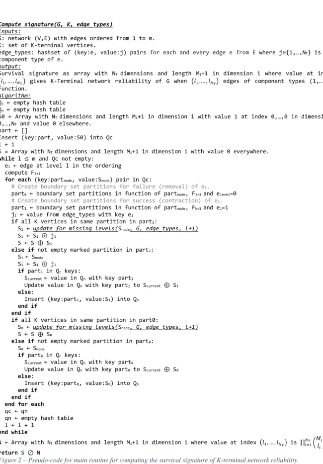
The pseudo-code for the main algorithm and a sub-routine it uses are shown in Figure 2 and Figure 3 respectively. The BDD construction procedure then follows that from Hermann and Soh (Herrmann et al., 2009) using network edge factorisation and boundary set partitions to identify isomorphic BDD nodes. However, a state vector count array (representing Φ̅ from Eqn. 3) is computed and stored for each BDD ite node and for the network functioning instead of reliability values. An array is initially created with the value 0 everywhere and assigned to variable S. This array represents Φ̅ corresponding to the network functioning (i.e. existence of a path through working edges between all K terminal nodes) and is updated during the edge factorisation process. A second array is also created with value 1 at index 0,…,0 in dimensions 0,…,NT and value 0 elsewhere, this is assigned to variable S0 and represents Φ̅ for the BDD
root node. The state vector count array operations that were defined above are then utilised by the algorithm during the edge factorisation process to compute the arrays representing Φ̅ for each ite node. The shift-j operation is used to update an array from the parent node to account for an additional component of type j that functions in the edge factorisation, whilst the elementwise addition operation is used to add the state vector count from a parent BDD node to that of a child node. When the edge factorisation results in the certain connection of the K terminal nodes, the array containing the state vector counts from the parent BDD node is first updated to account for the possible functioning or failed state of each edge at higher levels in the BDD since they do not influence the reliability of the network given the states of the already decided edges. This is performed by the sub-routine given in Figure 3, and the updated array is then added to the array for the state vector counts for the terminal 1 node. Once the edge factorisation is complete or no new child nodes were created from the BDD nodes at a level, the final operation in the main algorithm is to use the elementwise division operation to normalise the final state vector count Φ̅ corresponding to the network functioning by an array representing |𝑆𝑙1,…,𝑙
𝑁𝑇|, which is computed from the shape of the survival signature array, to
obtain the array representing the final survival signature Φ for the K-terminal network reliability. In the case of 𝑁𝑇 = 1, the simple transformation from Eqn. 6 can be used to compute
Compute signature(G, K, edge_types) inputs:
G: network (V,E) with edges ordered from 1 to m. K: set of K-terminal vertices.
edge_types: hashset of (key:e, value:j) pairs for each and every edge e from E where j∈{1,…,NT} is the component type of e.
output:
Survival signature as array with NT dimensions and length Mi+1 in dimension i where value at index (𝑙1, … , 𝑙𝑁𝑇) gives K-Terminal network reliability of G when (𝑙1, … , 𝑙𝑁𝑇) edges of component types (1,…,NT)
function.
algorithm:
Qc ← empty hash table Qn ← empty hash table
S0 ← Array with NT dimensions and length Mi+1 in dimension i with value 1 at index 0,…,0 in dimensions 0,…,NT and value 0 elsewhere.
part ← []
Insert (key:part, value:S0) into Qc l ← 1
S = Array with NT dimensions and length Mi+1 in dimension i with value 0 everywhere.
while l ≤ m and Qc not empty:
el ← edge at level l in the ordering compute Fl+1
for each (key:partnode, value:Snode) pair in Qc:
# Create boundary set partitions for failure (removal) of el.
part0 ← boundary set partitions in function of partnode, Fl+1 and elevel=0 # Create boundary set partitions for success (contraction) of el.
part1 ← boundary set partitions in function of partnode, Fk+1 and el=1 jl ← value from edge_types with key el
if all K vertices in same partition in part1:
S1 ← update for missing levels(Snode, G, edge_types, l+1) S1 ← S1 ⊛ jl
S ← S ⊕ S1
else if not empty marked partition in part1: S1 ← Snode
S1 ← S1 ⊛ jl
if part1 in Qn keys:
Scurrent ← value in Qn with key part1
Update value in Qn with key part1 to Scurrent ⊕ S1 else:
Insert (key:part1, value:S1) into Qn end if
end if
if all K vertices in same partition in part0:
S0 ← update for missing levels(Snode, G, edge_types, l+1) S ← S ⊕ S0
else if not empty marked partition in part0: S0 ← Snode
if part0 in Qn keys:
Scurrent ← value in Qn with key part0
Update value in Qn with key part0 to Scurrent ⊕ S0 else:
Insert (key:part0, value:S0) into Qn end if
end if end for each
qc ← qn
qn ← empty hash table l ← l + 1
end while
N ← Array with NT dimensions and length Mi+1 in dimension i where value at index (𝑙1, … , 𝑙𝑁𝑇) is ∏ (
𝑀𝑖
𝑙𝑖) 𝑁𝑇 𝑖=1
return S ⊘ N
update for missing levels(S, G, edge_types, from_level)
inputs:
S: Array with NT dimensions and length Mi+1 in dimension i that is to be updated.
G: network (V,E) with edges ordered from 1 to m.
edge_types: hashset of (key:e, value:j) pairs for each and every edge e from E where 𝑗 ∈ (𝑙1, … , 𝑙𝑁𝑇) is the component type of e.
from_level: the first missing level in the BDD.
output:
Array with NT dimensions and length Mi+1 in dimension i that represents S after updating for
edges at the missing levels.
algorithm:
for n from start_level to m: en ← edge at n in the ordering
jn ← value from edge_types with key en
S ← S ⊕ (S ⊛ jn)
end for return S
Figure 3 – Pseudo-code for sub-routine used by algorithm from Figure 2 to update array for missing levels in BDD.
Computational Complexity
Theorem: The computational complexity of the algorithm is 𝑂 (𝑚. 2𝐹𝑚𝑎𝑥. 𝐵
𝐹𝑚𝑎𝑥. (𝐹𝑚𝑎𝑥 +
(𝑚
𝑵𝑻) 𝑵𝑻
)), where 𝐹𝑚𝑎𝑥 is the maximum size of the boundary set and 𝐵𝐹𝑚𝑎𝑥 is the Bell number of 𝐹𝑚𝑎𝑥.
Proof: The number of BDD nodes at level 𝑙 is bounded by the theoretical maximum number of marked partitions which is given by 2𝐹𝑚𝑎𝑥. 𝐵
𝐹𝑚𝑎𝑥 (Hardy et al., 2007), whilst the size of a
signature array is bounded by (𝑚
𝑵𝑻+ 1) 𝑵𝑻
(Reed, 2017). For each BDD node, the two corresponding child node partitions for level 𝑙 + 1 must be computed which is O(|𝐹𝑙|) (Hardy et al., 2007) and the signatures corresponding to each of these partitions are updated through a small number of elementwise addition and shift-j array operations for which the complexity is approximately proportional to the number of array elements and therefore O ((𝑚
𝑵𝑻+ 1) 𝑵𝑻
). The computation time complexity is therefore 𝑂 (𝑚. 2𝐹𝑚𝑎𝑥. 𝐵
𝐹𝑚𝑎𝑥. (𝐹𝑚𝑎𝑥 + ( 𝑚 𝑵𝑻)
𝑵𝑻
)) whilst the memory complexity is 𝑂 (2𝐹𝑚𝑎𝑥. 𝐵
𝐹𝑚𝑎𝑥. ( 𝑚 𝑵𝑻)
𝑵𝑻
) since signature arrays are stored at a maximum of two levels of the BDD at any time.
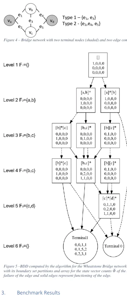
2.3.Example for Wheatstone bridge network
To illustrate the algorithm, it was applied to the Wheatstone bridge network shown in Figure 4 that has 5 edges of 2 component types. The BDD computed by the algorithm with edges ordered 𝑒1 < 𝑒2 < 𝑒3 < 𝑒4 < 𝑒5, where each ite node is labelled with its boundary set partitions and
array for the state vector counts (representing Φ̅ from Eqn. 3) of the survival signature, is shown in Figure 5. The terminal 1 node is labelled with the array representing Φ̅ for the network functioning.
va vb vc vd e1 e2 e5 e4 e3 Type 1 – {e1, e3} Type 2 - {e2,e4, e5}
Figure 4 – Bridge network with two terminal nodes (shaded) and two edge component types.
Figure 5 –BDD computed by the algorithm for the Wheatstone Bridge network from Figure 4, where each node is labelled with its boundary set partitions and array for the state vector counts 𝛷̅ of the survival signature. Dashed edges represent failure of the edge and solid edges represent functioning of the edge.
3. Benchmark Results
The algorithm introduced in the preceding section was applied to the computation of the system and survival signatures for 11 different K-terminal network reliability problems that have been
previously used for benchmarking algorithms in the literature. Since the problems from the literature all assume a single component type for the edges, additional variations of each problem were created that have two and three component types for the edges with an approximately equal number of components of each type.
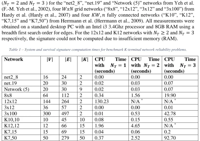
Table 1 shows the times for the computation of the system (𝑁𝑇 = 1 ) and survival signatures (𝑁𝑇 = 2 and 𝑁𝑇 = 3 ) for the “net2_8”, “net.19” and “Network (5)” networks from Yeh et al. (F.-M. Yeh et al., 2002), four 𝑊𝑥𝑁 grid networks (“8x8”, “12x12”, “3x12” and “3x100”) from Hardy et al. (Hardy et al., 2007) and four 𝐾𝑊, 𝑛 fully connected networks (“K10”, “K12”, “K7,15” and “K7,50”) from Herrmann et al. (Herrmann et al., 2009). All measurements were obtained on a standard desktop PC with an Intel i3 3.4Ghz processor and 8GB RAM using a breadth first search order for edges. For the 12x12 and K12 networks with 𝑁𝑇 ≥ 2 and 𝑁𝑇 = 3 respectively, the signature could not be computed due to insufficient memory (RAM).
Table 1 – System and survival signature computation times for benchmark K-terminal network reliability problems.
Network |𝑽| |𝑬| |𝑲| CPU Time
with 𝑵𝑻= 𝟏 (seconds) CPU Time with 𝑵𝑻= 𝟐 (seconds) CPU Time with 𝑵𝑻 = 𝟑 (seconds) net2_8 16 24 2 0.00 0.00 0.00 net.19 20 30 2 0.02 0.03 0.07 Network (5) 20 30 9 0.02 0.03 0.07 8x8 64 112 2 0.34 1.56 19.90 12x12 144 264 2 130.23 N/A * N/A * 3x12 36 57 2 0.00 0.00 0.01 3x100 300 497 2 0.01 0.53 42.78 K10,10 10 45 10 0.08 0.15 0.55 K12,12 12 66 15 1.96 4.65 N/A * K7,15 15 69 15 0.04 0.06 0.2 K7,50 50 279 50 0.37 2.52 92.70
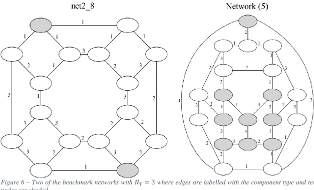
The 𝑁𝑇 = 3 variations of the “net2_8” and “Network (5)” networks are shown in Figure 6 and
their computed survival signatures are given in Appendix A.
Figure 6 – Two of the benchmark networks with 𝑁𝑇= 3 where edges are labelled with the component type and terminal nodes are shaded.
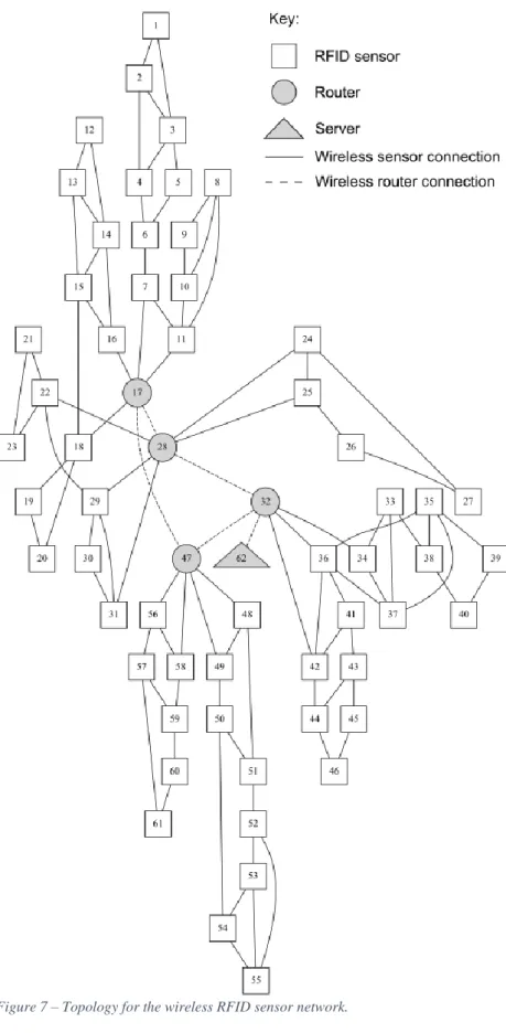
4. Application to analysis of the reliability of a RFID wireless sensor network This section describes the application of the algorithm to analyse reliability of a radio-frequency identification (RFID) sensor network at an underground mine. The network enables the location of personnel and mobile assets fitted with RFID tags to be tracked as they operate within the mine, increasing productivity and safety. RFID sensors and wireless routers are located strategically within the production areas of the mine and communicate with one another via short-range radio link to form a wireless mesh network. One of the routers is connected via wireless connection to a server that forms part of a wired network. When an RFID tag passes within range of a RFID sensor, a data packet containing the unique ID codes belonging to the tag and sensor along with the current time is generated by the sensor and sent over the wireless network to the server. The transmission protocol used ensures that a data packet generated by a sensor will reach the server if there exists at least one path between the sensor and the server through available node to node wireless connections. On receipt of a data packet, the server updates the last known location of the person or asset, which can then be viewed by mining staff on computer terminals connected to the server via the wired network. The topology of the wireless network, comprising 62 nodes (including 57 sensor nodes) and 96 wireless network connections between nodes, is shown in Figure 7. The wireless network connections between nodes in the network may temporarily fail due to radio-frequency (RF) interference created by machinery and equipment used in the mine, such as electric motors and personal dust monitors. In such cases, the nodes will attempt to re-establish the connection until it is restored. Failures of the nodes themselves (sensors, routers and the server) are negligible in comparison and are not considered in the analysis.
Figure 7 – Topology for the wireless RFID sensor network.
The level of the overall RF interference in the mine varies depending on the current activities and its normalised value, such that a value of 0 represents the minimum level of interference and a value of 1 represents the maximum level, is modelled as a random variable with a Beta distribution with shape parameters 3.8 and 5.3, as shown in Figure 8.
Figure 8- Plot of the probability density function (PDF) for the normalised level of RF interference in the mine.
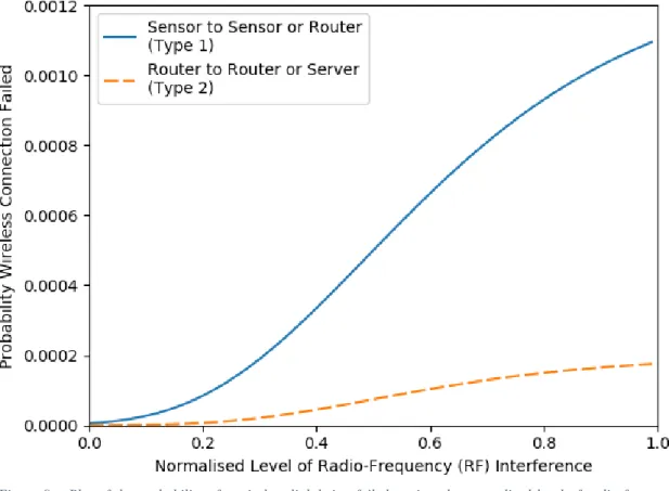
A wireless connection between a sensor and a sensor or router is denoted as a type 1 connection and the probability it is failed, 𝐹1, is modelled by the following Gompertz function of the
normalised level of RF interference in the mine 𝑧:
𝐹1(𝑧)= 0.0013𝑒−5.5𝑒 −3.5𝑧
Whilst a wireless connection between a router and a router or the server is denoted as a type 2 connection and the probability it is failed, 𝐹2, is modelled by the following Gompertz function
of the normalised level of RF interference in the mine 𝑧:
𝐹2(𝑧)= 0.0002𝑒−7.7𝑒 −4.1𝑧
There are 91 type 1 wireless connections and 5 type 2 wireless connections in the network. The parameters in the two failure probability models differ due to the different technologies used for the two types of wireless connection. Figure 9 shows a plot of the probability that each type of wireless connection is failed against the normalised level of RF interference in the mine.
Figure 9 – Plot of the probability of a wireless link being failed against the normalised level of radio-frequency (RF) interference in the mine.
The aim of the analysis is to determine the reliability of the simultaneous availability of a path along functioning wireless connections between a specified subset of the RFID sensors in the network and the server at a random time. This is therefore a K-terminal reliability problem where the K terminal nodes consist of the server and the subset of sensor nodes. The reliability of the connection between the server and each of the following three subsets of sensors from Figure 7 will be considered: all sensors, sensors numbered 48 to 61 (these sensors cover a single production area at the mine) and sensor 1.
Due to the common dependence between the failure probabilities of wireless connections and the level of RF interference in the mine, algorithms that assume independent edge failures, such as (Hardy et al., 2007; Herrmann et al., 2009), are unsuitable. However, it follows from the modelling assumptions that the failure events of edges representing wireless connections of the same type are exchangeable dependent whilst the failure events of edges representing wireless connections of different types are dependent. A survival signature for the network with two component types can therefore be computed for each of these three cases using the algorithm that was introduced in Section 2.2 of this paper (these signatures are given in Appendix A). The computation of each signature took approximately 10 seconds on the computer used for the benchmark tests with a breadth first search edge ordering starting from the sensor node labelled 1 in Figure 7. The K-terminal reliability for the network at random time 𝑡, 𝑅𝑡, can then be calculated for each case from its survival signature Φ :
𝑅𝑡 = ∑ ∑ [Φ𝑙1,𝑙2𝑃(𝐶𝑡 1= 𝑙 1, 𝐶𝑡2= 𝑙2)] 5 𝑙2=0 91 𝑙1=0 (10)
The probability that exactly 𝑙1 and 𝑙2 of the type 1 and type 2 wireless connections,
respectively, are failed in the network at random time 𝑡 is given by:
𝑃(𝐶𝑡1= 𝑙1, 𝐶𝑡2= 𝑙2) = ( 91 𝑙1) ( 5 𝑙2) ∫ 𝑓(𝑧)[𝐹1(𝑧)] 91−𝑙1[1 − 𝐹 1(𝑧)]𝑙1[𝐹2(𝑧)]5−𝑙2[1 − 𝐹2(𝑧)]𝑙2𝑑𝑧 1 0 (11)
where 𝑓(𝑧) is the probability density function of the normalised level of RF interference in the mine. This integral was approximated numerically for each combination of 𝑙1 and 𝑙2 using the tanh-sinh quadrature algorithm (Bailey, Jeyabalan, & Li, 2005) and the computed values are given in Appendix A. The following K-terminal network reliabilities for the three sensor nodes subset cases were computed: 0.999558 for the all sensors case, 0.999944 for the sensors numbered 48 to 61 case and 0.999565 for the sensor 1 case.
The failures of wireless network connections are conditionally independent given that the normalised level of RF interference in the mine is known at time 𝑡. Therefore, the probability that exactly 𝑙1 and 𝑙2 of the type 1 and type 2 wireless connections, respectively, are failed in
the network at time 𝑡 when the normalised level of RF interference is 𝑧 is given by:
𝑃(𝐶𝑡1= 𝑙1, 𝐶𝑡2= 𝑙2) = ( 91 𝑙1) ( 5 𝑙2) [𝐹1(𝑧)] 91−𝑙1[1 − 𝐹 1(𝑧)]𝑙1[𝐹2(𝑧)]5−𝑙2[1 − 𝐹2(𝑧)]𝑙2 (11)
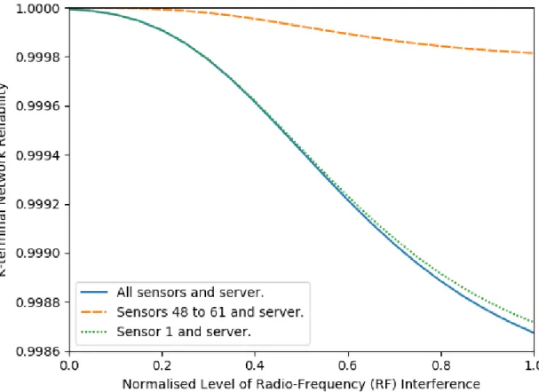
Figure 10 shows a plot of the K-terminal reliability against the normalised level of RF interference for the three different sets of terminal nodes. Note that the plotted reliability values could also have been determined from the K-terminal reliability network algorithms that assume independent edge failures. However, the advantage of the signature approach is that repeating the edge factorisation and BDD construction process was not required. Instead, the reliabilities were calculated directly from the signatures for the different edge failure probabilities, making it much more computationally efficient.
Figure 10 – Plot of the K-terminal network reliability against the normalised level of RF interference for the network in Figure 7 for three different sets of terminal nodes.
5. Discussion and Conclusions
Previous algorithms for the computation of system and survival signatures for networks required the derivation of cut-set or path sets as an intermediate step which is computationally infeasible when the network is large and complex. A new algorithm was presented in this paper that utilises binary decision diagrams, boundary set partition sets and simple array operations to efficiently compute signatures through a factorisation of the network edges. The computation times for a set of benchmark problems from the literature demonstrate the efficiency of the algorithm, in many cases it was able to compute the signatures within a few seconds on a standard PC. The results for the 3x100 grid network show that signatures for even very large networks, in this case with 497 edges, can be computed in reasonable times provided that the maximum size of the boundary set is small. As expected, computation times are greater for networks with greater numbers of edges, greater boundary set sizes and greater numbers of signature elements.
The analysis of a RFID sensor network from an underground mine using the new algorithm provided an example of the practical applications. Using the survival signatures computed for the network, K-terminal reliability values were obtained for exchangeable but non-independent edge failures. K-terminal reliability values for the network were also computed for multiple edge failure probabilities using the signatures, eliminating the need for repetition of the edge factorisation and BDD construction process.
It was not possible to compute the signatures for a small number of the benchmark problems due to the memory requirement exceeding the available resources on the computer used. The huge memory requirement in these cases was due to a combination of a signature with a large number of elements, resulting from the number of edges belonging to each component type, and a large maximum BDD width resulting from the edge factorisation. Further research is needed on the development of algorithms to make it feasible to compute survival signatures for these cases. The presented algorithm is limited to the computation of signatures for K-terminal network reliability of undirected networks with unreliable edges and perfectly reliable vertices. The development of similar methods for networks with unreliable vertices and directed edges is another area for future work.
6. References
Aslett, L. J. M., Coolen, F. P. A., & Wilson, S. P. (2015). Bayesian Inference for Reliability of Systems and Networks Using the Survival Signature. Risk Analysis, 35(9), 1640–1651. https://doi.org/10.1111/risa.12228
Asthana, S., King, O. D., Gibbons, F. D., & Roth, F. P. (2004). Predicting Protein Complex Membership Using Probabilistic Network Reliability. Genome Research, 14, 1170–1175. https://doi.org/10.1101/gr.2203804
Bailey, D. H., Jeyabalan, K., & Li, X. S. (2005). A comparison of three high-precision quadrature schemes. Experimental Mathematics, 14(3), 317–329. https://doi.org/10.1080/10586458.2005.10128931
Ball, M. O. (1986). Computational Complexity of Network Reliability Analysis: An Overview. IEEE Transactions on Reliability, 35(3), 230–239. https://doi.org/10.1109/TR.1986.4335422
Block, H., Dugas, M. R., & Samaniego, F. J. (2006). Characterizations of the Relative Behavior of Two Systems via Properties of Their Signature Vectors. In N. Balakrishnan, J. M. Sarabia, & E. Castillo (Eds.), Advances in Distribution Theory, Order Statistics, and Inference (pp. 279–289). Boston, MA, MA: Birkh{ä}user Boston. https://doi.org/10.1007/0-8176-4487-3_18
Boland, P. J., & Samaniego, F. J. (2004). The Signature of a Coherent System and Its Applications in Reliability. In R. Soyer, T. A. Mazzuchi, & N. D. Singpurwalla (Eds.), Mathematical Reliability: An Expository Perspective (pp. 3–30). Boston, MA, MA: Springer US. https://doi.org/10.1007/978-1-4419-9021-1_1
Boland, P. J., Samaniego, F. J., & Vestrup, E. M. (2003). Linking Dominations and Signatures in Network Reliability Theory. In B. H. Lindqvist & K. A. Doksum (Eds.), Mathematical and Statistical Methods in Reliability. Singapore: World Scientific.
Botev, Z. I., L’Ecuyer, P., Rubino, G., Simard, R., & Tuffin, B. (2013). Static Network Reliability Estimation via Generalized Splitting. INFORMS Journal on Computing, 25(1), 56–71. https://doi.org/10.1287/ijoc.1110.0493
Brecmt, T. B., & Colbourn, C. J. (1988). Lower bounds on two terminal network reliability. Discrete Applied Mathematics, 21, 185–198.
Bryant, R. E. (1986). Graph-Based Algorithms for Boolean Function Manipulation. IEEE
Transactions on Computers, C-35(8), 677–691.
https://doi.org/10.1109/TC.1986.1676819
Carlier, J., & Lucet, C. (1996). A decomposition algorithm for network reliability evaluation. Discrete Applied Mathematics, 65(1–3), 141–156. https://doi.org/10.1016/0166-218X(95)00032-M
Coolen, F. P. A., & Coolen-Maturi, T. (2012). Generalizing the Signature to Systems with Multiple Types of Components. In Complex Systems and Dependability (pp. 115–130). Springer Berlin Heidelberg. https://doi.org/10.1007/978-3-642-30662-4_8
Eryilmaz, S., Coolen, F. P. A., & Coolen-Maturi, T. (2018). Marginal and joint reliability importance based on survival signature. Reliability Engineering and System Safety, 172, 118–128. https://doi.org/10.1016/j.ress.2017.12.002
Fard, N. S., & Lee, T. H. (1999). Cutset enumeration of network systems with link and node failures. Reliability Engineering and System Safety, 65(2), 141–146. https://doi.org/10.1016/S0951-8320(98)00096-9
Hardy, G., Lucet, C., & Limnios, N. (2007). K-Terminal Network Reliability Measures With Binary Decision Diagrams. IEEE Transactions on Reliability, 56(3), 506–515. https://doi.org/10.1109/TR.2007.898572
Herrmann, J. U., Soh, S., & Model, A. N. (2009). A Memory Efficient Algorithm for Network Reliability. In 15th Asia-Pacific Conf. Communications (APCC2009) (pp. 703–707). https://doi.org/10.1109/APCC.2009.5375505
Imai, H., Serine, K., & Imai, K. (1999). Computational investigations of all-terminal network reliability via BDDs. IEICE Transactions on Fundamentals of Electronics, Communications and Computer Sciences, E82–A(5), 714–721.
Jane, C. C., Shen, W. H., & Laih, Y. W. (2009). Practical sequential bounds for approximating two-terminal reliability. European Journal of Operational Research, 195(2), 427–441. https://doi.org/10.1016/j.ejor.2008.02.022
Manzi, E., Labbé, M., Latouche, G., & Maffioli, F. (2001). Fishman’s sampling plan for computing network reliability. IEEE Transactions on Reliability, 50(1), 41–46. https://doi.org/10.1109/24.935016
McAssey, M. P., & Samaniego, F. J. (2014). On uniformly optimal networks: A reversal of fortune? Communications in Statistics - Theory and Methods, 43(10–12), 2452–2467. https://doi.org/10.1080/03610926.2013.792353
Michelena, N. F., & Papalambros, P. Y. (1994). A Network Reliability Approach to Optimal Decomposition of Design Problems. Journal of Mechanical Design, 2(September 1995), 195–204. https://doi.org/10.1115/1.2826697
Niu, Y. F., & Shao, F. M. (2011). A practical bounding algorithm for computing two-terminal reliability based on decomposition technique. Computers and Mathematics with Applications, 61(8), 2241–2246. https://doi.org/10.1016/j.camwa.2010.09.033
Page, L. B., & Perry, J. E. (1989). Reliability of direct networks using the factoring theorem. IEEE Transactions on Reliability, 38(5), 556–562. Retrieved from http://ieeexplore.ieee.org/ielx1/24/1755/00046479.pdf?tp=&arnumber=46479&isnumbe r=1755
Patelli, E., Feng, G., Coolen, F. P. A., & Coolen-Maturi, T. (2017). Simulation methods for system reliability using the survival signature. Reliability Engineering and System Safety, 167, 327–337. https://doi.org/10.1016/j.ress.2017.06.018
Provan, J. S. (1986). The Complexity of Reliability Computations in Planar and Acyclic Graphs. SIAM Journal on Computing, 15(3), 694–702. https://doi.org/10.1137/0215050 Rauzy, A. (1993). New algorithms for fault trees analysis. Reliability Engineering and System
Safety, 40, 203–211.
Reed, S. (2017). An efficient algorithm for exact computation of system and survival signatures using binary decision diagrams. Reliability Engineering and System Safety, 165(March), 257–267. https://doi.org/10.1016/j.ress.2017.03.036
Samaniego, F. J. (1985). On Closure of the IFR Class Under Formation of Coherent Systems. IEEE Transactions on Reliability, R-34(1), 69–72. https://doi.org/10.1109/TR.1985.5221935
Samaniego, F. J. (2007). System Signatures and their Applications in Engineering Reliability (Vol. 110). Boston, MA: Springer US. https://doi.org/10.1007/978-0-387-71797-5 Samaniego, F., & Navarro, J. (2016). On comparing coherent systems with heterogeneous
components. Advances in Applied Probability, 48(1), 88–111. Retrieved from http://projecteuclid.org/euclid.aap/1457466157
Shannon, C. E. (1938). A symbolic analysis of relay and switching circuits. Transactions of the American Institute of Electrical Engineers, 57(12), 713–723. https://doi.org/10.1109/T-AIEE.1938.5057767
Theologou, O. R., & Carlier, J. G. (1991). Factoring & Reductions for Networks with Imperfect Vertices. IEEE Transactions on Reliability, 40(2), 210–217. https://doi.org/10.1109/24.87131
Valiant, L. G. (1979). The Complexity of Enumeration and Reliability Problems. SIAM Journal on Computing, 8(3), 410–421. https://doi.org/10.1137/0208032
Wood, R. K. (1986). Factoring Algorithms for Computing K-Terminal Network Reliability. IEEE Transactions on Reliability, 35(3), 269–278. https://doi.org/10.1109/TR.1986.4335431
Yeh, F.-M., Lu, S.-K., & Kuo, S.-Y. (2002). OBDD-Based evaluation of k-terminal network
reliability. IEEE TRANSACTIONS ON RELIABILITY, 51(4).
https://doi.org/10.1109/TR.2002.804736
Yeh, W. C. (2006). A simple algorithm to search for all MCs in networks. European Journal of Operational Research, 174(3), 1694–1705. https://doi.org/10.1016/j.ejor.2005.02.047
7. Appendix A. Supplementary Data
The survival signatures computed for “net2_8” and “Network (5)” with 𝑁𝑇 = 3 from the
benchmark networks presented in Section 3 along with the survival signatures and wireless connection failure probabilities from the example sensor network presented in Section 4 are provided as a Microsoft Excel spreadsheet file.