Model selection and model averaging in the presence of missing values

Glasgow Theses Service

http://theses.gla.ac.uk/

[email protected]

Gopal Pillay, Khuneswari (2015)

Model selection and model

averaging in the presence of missing values.

PhD thesis.

http://theses.gla.ac.uk/6834/

Copyright and moral rights for this thesis are retained by the author

A copy can be downloaded for personal non-commercial research or study

This thesis cannot be reproduced or quoted extensively from without first

obtaining permission in writing from the Author

The content must not be changed in any way or sold commercially in any format

or medium without the formal permission of the Author

When referring to this work, full bibliographic details including the author, title,

awarding institution and date of the thesis must be given

MODEL SELECTION AND MODEL

AVERAGING IN THE PRESENCE OF

MISSING VALUES

by

KHUNESWARI GOPAL PILLAY

A thesis submitted in partial fulfillment for the degree of Doctor of Philosophy

in the

SCHOOL OF MATHEMATICS AND STATISTICS

I, KHUNESWARI GOPAL PILLAY, declare that this thesis titled, ‘Model selection and model averaging in the presence of missing values’ and the work presented in it are my own. I confirm that:

This work was done wholly or mainly while in candidature for a research degree

at this University.

Where any part of this thesis has previously been submitted for a degree or any

other qualification at this University or any other institution, this has been clearly stated.

Where I have consulted the published work of others, this is always clearly

at-tributed.

Where I have quoted from the work of others, the source is always given. With

the exception of such quotations, this thesis is entirely my own work.

I have acknowledged all main sources of help.

Where the thesis is based on work done by myself jointly with others, I have made

clear exactly what was done by others and what I have contributed myself.

Signed:

Date:

Model averaging has been proposed as an alternative to model selection which is in-tended to overcome the underestimation of standard errors that is a consequence of model selection. Model selection and model averaging become more complicated in the presence of missing data. Three different model selection approaches (RR, STACK and M-STACK) and model averaging using three model-building strategies (non-overlapping variable sets, inclusive and restrictive strategies) were explored to combine results from multiply-imputed data sets using a Monte Carlo simulation study on some simple linear and generalized linear models. Imputation was carried out using chained equations (via the ”norm” method in the R package MICE). The simulation results showed that the STACK method performs better than RR and M-STACK in terms of model selection and prediction, whereas model averaging performs slightly better than STACK in terms of prediction. The inclusive and restrictive strategies perform better in terms of predic-tion, but non-overlapping variable sets performs better for model selection. STACK and model averaging using all three model-building strategies were proposed to combine the results from a multiply-imputed data set from the Gateshead Millennium Study (GMS). The performance of STACK and model averaging was compared using mean square error of prediction (MSE(P)) in a 10% cross-validation test. The results showed that STACK using an inclusive strategy provided a better prediction than model averaging. This coincides with the results obtained through a mimic simulation study of GMS data. In addition, the inclusive strategy for building imputation and prediction models was better than the non-overlapping variable sets and restrictive strategy. The presence of highly correlated covariates and response is believed to have led to better prediction in this particular context. Model averaging using non-overlapping variable sets performs better only if an auxiliary variable is available. However, STACK using an inclusive strategy performs well when there is no auxiliary variable available. Therefore, it is advisable to use STACK with an inclusive model-building strategy and highly correlated covariates (where available) to make predictions in the presence of missing data. Alternatively, model averaging with non-overlapping variables sets can be used if an auxiliary variable is available.

First of all, I would like to thank God for his blessings that enabled me to complete my studies by providing opportunities and insights for conducting the research. Next, I would like to take this opportunity to express my gratitude to my supervisor Professor John H. McColl for his advice, guidance, constructive comments and immerse contribu-tion to my final piece of work and his invaluable help and assistance in the complecontribu-tion of this project. All his efforts are deeply appreciated and would not be forgotten. I would also like to thank Professor Charlotte Wright and the Gateshead Millennium Study Core Team for giving approval to use the Gateshead Millennium Study data for my research. I would like to thank my beloved husband Mohana Kanapathy for his support, guidance, love, sacrifice and motivation throughout my research duration. I would also like to thank my beloved parents Gopal Pillay and Vasantha Kumari, my brothers Thinesh and Vijayan for their support, love and motivation throughout my research duration. I would like to thank my sister Kogilavani, my friends and colleagues for their encouragement and motivation.

I would like to thank Ministry of Education Malaysia (MOE) and Universiti Tun Hussein Onn Malaysia (UTHM) for their financial support and guidance throughout my research duration. I would like to thank Professor Zainodin Hj. Jubok from University Malaysia Sabah for his support and motivation.

Lastly, I wish to thank all lecturers, staff and friends in School of Mathematic and Statistics and College of Science and Engineering who helped me in giving guidance and support throughout my years at University of Glasgow.

Declaration of Authorship i

Abstract iii

Acknowledgements iv

List of Figures ix

List of Tables xiii

Abbreviations xvi Symbols xvii 1 Introduction 1 1.1 Research Motivations . . . 2 1.2 Research Objectives . . . 3 1.3 Thesis Outline . . . 4 2 Methodology 6 2.1 Missing Data . . . 6

2.2 Statistical Approaches to Analyze Missing Data . . . 7

2.2.1 Complete-case analysis . . . 7

2.2.2 Single imputation . . . 8

2.2.3 Hot deck imputation . . . 9

2.2.4 EM algorithm . . . 10

2.2.5 Multiple imputation and Rubin’s Rules . . . 11

2.2.6 Chained equations . . . 13

2.3 Software Packages for Imputation . . . 14

2.3.1 Multiple imputation (MI) . . . 15

2.3.2 Multivariate imputation by chained equations (MICE) . . . 15

2.4 Model Selection Criteria . . . 18

2.4.1 Stepwise selection of variables . . . 20

2.4.2 All subset regression . . . 21

2.4.3 Kullback-Leibler distance . . . 22 v

2.4.4 Akaike’s information criterion (AIC) and AICc . . . 23

2.4.5 Bayesian information criterion (BIC) . . . 26

2.4.6 Model selection criteria for missing data . . . 27

2.4.7 Comparison of model selection criteria . . . 29

2.5 Model Averaging . . . 30

2.6 Bias and Mean Squared Error of Prediction . . . 32

2.6.1 Bias . . . 32

2.6.2 Mean squared error of prediction . . . 33

2.7 Multicollinearity . . . 33

2.7.1 Consequences of multicollinearity . . . 34

3 Review of Model Selection and Model Averaging in the Presence of Missing Values 37 3.1 Model Selection in the Presence of Missing Values . . . 37

3.1.1 Model selection strategies . . . 38

3.1.2 Model selection criteria . . . 46

3.1.3 Strategies for building an imputation model . . . 49

3.2 Model Averaging in the Presence of Missing Values . . . 52

3.3 Summary . . . 56

4 Comparison between Model Selection and Model Averaging 63 4.1 Design of Simulation . . . 63

4.1.1 Linear model and Logistic regression . . . 64

4.1.2 Imputation and prediction models . . . 65

4.1.3 Test values . . . 67

4.1.4 Choice of imputation package and method . . . 68

4.2 Results . . . 71

4.2.1 Linear regression with non-overlapping variable sets . . . 71

4.2.2 Linear regression with restrictive and inclusive strategies . . . 81

4.2.3 Logistic regression with non-overlapping variable sets . . . 85

4.2.4 Logistic regression with restrictive and inclusive Strategies . . . 89

4.3 Discussion and Conclusions . . . 91

5 The Implementation of Model Selection and Model Averaging using Multiple Imputation 95 5.1 Model Selection and Model Averaging for Multiple Imputation . . . 96

5.1.1 Rubin’s rules (RR) . . . 96

5.1.2 STACK . . . 97

5.1.3 M-STACK . . . 98

5.1.4 Model Averaging for Multiple Imputation . . . 98

5.2 Design of Simulation and Results . . . 99

5.2.1 Linear regression . . . 99

5.2.1.1 Rubin’s Rules (RR) using non-overlapping variable sets for Linear regression . . . 99

5.2.1.2 STACK using non-overlapping variable sets for Linear regression . . . 103

5.2.1.3 M-STACK using non-overlapping variable sets for Linear regression . . . 106

5.2.1.4 Model averaging using non-overlapping variable sets for Linear regression . . . 109 5.2.1.5 Model selection (STACK) and model averaging using

re-strictive and inclusive strategies for Linear regression . . 113 5.2.2 Logistic regression . . . 118

5.2.2.1 Rubin’s Rules (RR) using non-overlapping variable sets for Logistic regression . . . 118 5.2.2.2 STACK using non-overlapping variable sets for Logistic

regression . . . 120 5.2.2.3 M-STACK using non-overlapping variable sets for

Logis-tic regression . . . 123 5.2.2.4 Model averaging using non-overlapping variable sets for

Logistic regression . . . 125 5.2.2.5 Model selection (STACK) and model averaging using

re-strictive and inclusive strategies for Logistic regression . . 128 5.3 Discussion and Conclusions . . . 131

6 Application of Model Selection and Model Averaging to the Gateshead

Millennium Study 135

6.1 Data Description of Gateshead Millennium Study . . . 135 6.2 Model-building and Results . . . 142 6.2.1 Complete case analysis . . . 143 6.2.2 Prediction of weight at school entry using multiple imputation . . 147 6.2.3 Prediction of weight at eight years using multiple imputation . . . 152 6.2.4 Prediction of weight Z-scores at eight years using multiple

impu-tation . . . 156 6.3 Gateshead Millennium Study Simulation Results . . . 161 6.4 Discussion and Conclusions . . . 163

7 Conclusion 166

7.1 Review of Objectives and Guidelines . . . 166 7.2 Research Contributions . . . 168 7.3 Limitations and Recommendations for Further Work . . . 169

A R-script for Model averaging using Multiple Imputation for Linear

Regression 171

B R-script for Model Selection (RR) using Multiple Imputation for

Lin-ear Regression 178

C R-script for Model Selection (M-STACK) using Multiple Imputation

for Linear Regression 186

D R-script for Model Selection (STACK) using Multiple Imputation for

Linear Regression 193

E R-script for Model Selection (STACK) using Multiple Imputation for

4.1 Bias and MSE for norm.nob and norm methods in package MICE for linear regression . . . 69 4.2 Bias and MSE for norm.nob and norm methods in package MICE for

logistic regression . . . 70 4.3 MSE(P) for best model selected via AICc and BIC for different sample

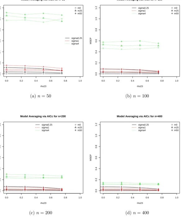
sizes and linear regression . . . 77 4.4 MSE(P) for model averaging via AICc and BIC for eachρ23,σε, missing

percentages and all sample sizes for linear regression . . . 80 4.5 Comparison between model averaging and model selection for non-overlapping

variable sets via AICc for each ρ23, σε, missing percentages and sample

sizes,n= 50 andn= 400 for linear regression . . . 81 4.6 Comparison between model averaging and model selection for restrictive

strategy via AICc for eachρ23,σε, missing percentages and sample sizes,

n= 50 andn= 400 for linear regression . . . 82 4.7 Comparison between model averaging and model selection for inclusive

strategy via AICc for eachρ23,σε, missing percentages and sample sizes,

n= 50 andn= 400 for linear regression . . . 83 4.8 Comparison between all three model-building strategies for model

averag-ing and model selection for eachρ23,σε, missing percentages and sample

size (n= 50 and n= 400) for linear regression . . . 84 4.9 MSE(P) for best model selected and model averaging via AICc and BIC

for eachρ23, missing percentages and sample sizes (n=50 and n=400) for

logistic regression . . . 88 4.10 Comparison between model averaging and model selection for non-overlapping

variable sets via AICc for eachρ23, missing percentages and sample sizes

(n=50 and n=400)for logistic regression . . . 89 4.11 Comparison between model averaging and model selection for restrictive

and inclusive strategies via AICc for each ρ23, missing percentages and

sample sizes (n=50 and n=400) for logistic regression . . . 90 4.12 Comparison between all three model-building strategies for model

aver-aging and model se4lection for each ρ23, missing percentages and sample

size (n=50 and n=400)for logistic regression . . . 90 5.1 MSE(P) for selected best model using RR for each ρ23, σε, missing

per-centages and sample sizes for linear regression . . . 102 5.2 MSE(P) for best model selected via AICcusing STACK and non-overlapping

variable sets for eachρ23,σε, missing percentages and sample sizes for

lin-ear regression . . . 105

5.3 MSE(P) for best model selected via AICc using M-STACK for each ρ23,

σε, missing percentages and sample for linear regression . . . 108

5.4 Comparison between model selection methods for each ρ23, σε, missing

percentages andn= 100 for linear regression . . . 109 5.5 MSE(P) for model averaging via AICc for each ρ23, σε, missing

percent-ages and sample sizes for linear regression . . . 111 5.6 Comparison between model averaging and model selection (STACK) via

AICc for eachρ23,σε, missing percentages and sample sizes (n= 50 and

n= 400) for linear regression . . . 112 5.7 Comparison between single imputation and multiple imputation for model

averaging and model selection via AICc for each ρ23, σε = 1, missing

percentages and sample sizes for linear regression . . . 112 5.8 MSE(P) for best model selected via AICcusing STACK and the restrictive

strategy for each ρ23, σε, missing percentages and sample sizes (n = 50

and n= 400) for linear regression . . . 113 5.9 MSE(P) for best model selected via AICcusing STACK and the inclusive

strategy for each ρ23, σε, missing percentages and sample sizes (n = 50

and n= 400) for linear regression . . . 114 5.10 MSE(P) for model averaging via AICc using the restrictive strategy for

each ρ23,σε, missing percentages and sample sizes (n= 50 andn= 400)

for linear regression . . . 114 5.11 MSE(P) for model averaging via AICc using the inclusive strategy for

each ρ23,σε, missing percentages and sample sizes (n= 50 andn= 400)

for linear regression . . . 115 5.12 Comparison between all three model-building strategies for model

aver-aging and model selection (STACK) for multiply-imputed data sets for linear regression . . . 116 5.13 Comparison between single imputation and multiple imputation for model

averaging and model selection for eachρ23, missing percentages, n= 100

and error variances,σε= 1 and σε= 4 for linear regression . . . 117

5.14 MSE(P) for best model selected using RR for eachρ23, missing

percent-ages and sample sizes for logistic regression . . . 120 5.15 MSE(P) for for best model selected (STACK) and non-overlapping

vari-able sets for each ρ23, missing percentages and sample sizes for logistic

regression . . . 122 5.16 MSE(P) for for best model selected using M-STACK for eachρ23, missing

percentages and sample sizes for logistic regression . . . 124 5.17 Comparison between all three model selection methods (RR, M-STACK

and STACK) for each ρ23, missing percentages and n = 100 for logistic

regression . . . 125 5.18 MSE(P) for model averaging via AICcusing non-overlapping variable sets

for each ρ23, missing percentages and sample size for logistic regression . . 126

5.19 Comparison between model averaging and model selection (STACK) via AICc for each ρ23, missing percentages and sample sizes (n = 50 and

n= 400) for logistic regression . . . 127 5.20 Comparison between single imputation and multiple imputation for model

averaging and model selection via AICc for each ρ23, σε = 1, missing

5.21 MSE(P) for for best model selected using STACK and the restrictive and inclusive strategies for eachρ23, missing percentages and sample sizes for

logistic regression . . . 128 5.22 MSE(P) for model averaging via AICc using the restrictive and inclusive

strategies for each ρ23, missing percentages and sample sizes for logistic

regression . . . 129 5.23 Comparison between all three model-building strategies for model

aver-aging and model selection (STACK) for multiply-imputed data sets for logistic regression . . . 129 5.24 Comparison between single imputation and multiple imputation for model

averaging and model selection for eachρ23, missing percentages and

sam-ple size, n= 100 for logistic regression . . . 130 6.1 Weight at school entry and weight at eight years for boys and girls separately137 6.2 The relationship between birth weight and gestational age for both male

and female babies . . . 138 6.3 Relationship between the weight at school entry, weight at eight years

and the first year baby weights . . . 139 6.4 Weight Z-scores at eight years for both male and female children . . . 140 6.5 Relationship between the weight Z-scores at eight years and the first year

baby weights . . . 141 6.6 Distribution of imputed values for weight at school entry for male children

using non-overlapping, restrictive and inclusive strategies using multiple imputation . . . 147 6.7 Distribution of imputed values for first year baby’s weights for male babies

using non-overlapping and restrictive strategy using multiple imputation . 148 6.8 Distribution of imputed values for first year baby’s weights for male babies

using inclusive strategy using multiple imputation . . . 149 6.9 Residuals for male children using inclusive strategy and model selection

criterion AICcusing multiple imputation for prediction of weight at school

entry . . . 150 6.10 Residuals for female children using inclusive strategy and model selection

criterion AICcusing multiple imputation for prediction of weight at school

entry . . . 152 6.11 Distribution of imputed values for weight at eight years for male children

using non-overlapping, restrictive and inclusive strategies using multiple imputation . . . 153 6.12 Residuals for male children using non-overlapping variable sets and model

selection criterion, AICcusing multiple imputation for prediction of weight

at eight years . . . 154 6.13 Distribution of imputed values for weight at eight years for female children

using non-overlapping, restrictive and inclusive strategy using multiple imputation . . . 154 6.14 Residuals for female children using restrictive strategy and model selection

criterion, BIC using multiple imputation for prediction of weight at eight years . . . 156 6.15 Distribution of imputed values for weight Z-scores at eight years for male

children using non-overlapping, restrictive and inclusive strategies using multiple imputation . . . 157

6.16 Distribution of imputed values for first year baby’s weight Z-scores for male babies using non-overlapping and restrictive strategy using multiple imputation . . . 157 6.17 Distribution of imputed values for first year baby’s weight Z-scores for

male babies using inclusive strategy using multiple imputation . . . 158 6.18 Residuals for male children using non-overlapping variables sets and model

selection criterion, AICcusing multiple imputation for prediction of weight

Z-scores at eight years . . . 159 6.19 Residuals for female children using non-overlapping variable set and model

selection criterion, AICcusing multiple imputation for prediction of weight

Z-scores at eight years . . . 161 6.20 MSEP for model averaging and STACK via AICc using non-overlapping,

restrictive and inclusive strategies for GMS simulation using multiple im-putation . . . 163

2.1 Buit-in Imputation methods in MICE . . . 17

3.1 Review of Model Selection in the Presence of Missing Data . . . 59

3.2 Review of Model Averaging in the Presence of Missing Data . . . 62

4.1 All possible prediction models . . . 66

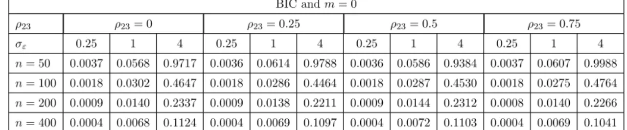
4.2 Number of times all possible models are selected via AICc and BIC in each of 1000 simulations for all the combinations of ρ23 when σε= 1 and m= 50 for linear regression . . . 72

4.3 Number of times all possible models are selected via AICc and BIC in each of 1000 simulations for all the combinations of ρ23 when σε= 4 and m= 0 for linear regression . . . 72

4.4 Number of times all possible models are selected via AICc and BIC in each of 1000 simulations for all the combinations of ρ23 when σε= 4 and m= 25 for linear regression . . . 73

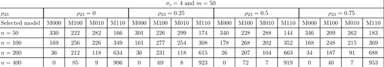
4.5 Number of times all possible models are selected via AICc and BIC in each of 1000 simulations for all the combinations of ρ23 when σε= 4 and m= 50 for linear regression . . . 74

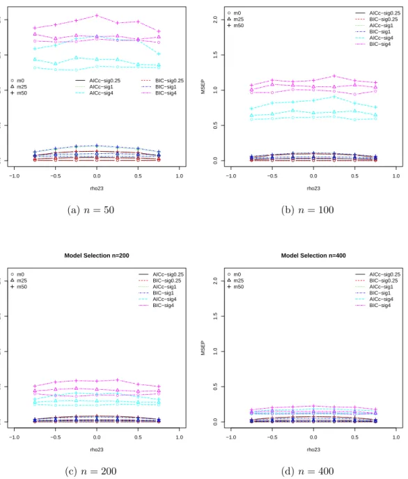
4.6 MSE(P) for best model selected via AICcand BIC whenm= 0 for linear regression . . . 74

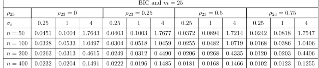
4.7 MSE(P) for best model selected via AICcand BIC whenm= 25 for linear regression . . . 75

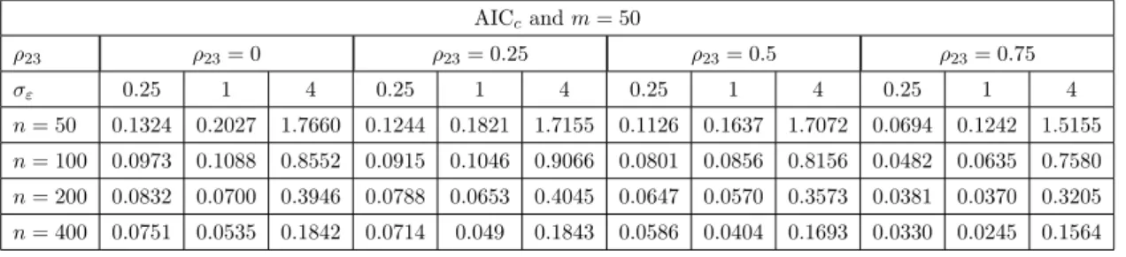
4.8 MSE(P) for best model selected via AICcand BIC whenm= 50 for linear regression . . . 76

4.9 MSE(P) for model averaging via AICc and BIC when m = 0 for linear regression . . . 78

4.10 MSE(P) for model averaging via AICc and BIC when m = 25 for linear regression . . . 78

4.11 MSE(P) for model averaging via AICc and BIC when m = 50 for linear regression . . . 79

4.12 Number of times all possible models are selected by AICc and BIC in each of 1000 simulations for all the combinations of ρ23 when m = 0 for logistic regression . . . 85

4.13 Number of times all possible models are selected by AICc and BIC in each of 1000 simulations for all the combinations of ρ23 when m= 25 for logistic regression . . . 86

4.14 Number of times all possible models are selected by AICc and BIC in each of 1000 simulations for all the combinations of ρ23 when m= 50 for logistic regression . . . 86

4.15 MSE(P) for best model selected via AICc and BIC for logistic regression . 87

4.16 MSE(P) for model averaging via AICc and BIC for logistic regression . . . 87

5.1 Number of times all possible models are selected in each of 1000 simula-tions for all the combinasimula-tions of ρ23 when n= 50 and σε = 1 using RR

for linear regression . . . 100 5.2 Number of times all possible models are selected in each of 1000

simula-tions for all the combinasimula-tions of ρ23,σε= 4 and sample size (n= 50 and

n= 100) using RR for linear regression . . . 100 5.3 Number of times all possible models are selected in each of 1000

simula-tions for all the combinasimula-tions ofρ23,σε= 4 and sample size (n= 200 and

n= 400) using RR for linear regression . . . 101 5.4 MSE(P) for selected best model for all the combinations of ρ23, missing

percentages, sample size and error variances (σε = 1 and σε = 4) using

RR for linear regression . . . 101 5.5 Number of times all possible models are selected via AICcin each of 1000

simulations for all the combinations ofρ23,σε= 4 and sample size (n= 50

and n= 100) using STACK for linear regression . . . 103 5.6 Number of times all possible models are selected via AICcin each of 1000

simulations for all the combinations ofρ23whenn= 200 andσε= 4 using

STACK for linear regression . . . 104 5.7 MSE(P) for selected best model via AICcfor all the combinations ofρ23,

missing percentages, sample size and error variances (σε= 1 and σε= 4)

using STACK for linear regression . . . 104 5.8 Number of times all possible models are selected via AICcin each of 1000

simulations for all the combinations ofρ23,σε= 4 and sample size (n= 50

and n= 100) using M-STACK for linear regression . . . 106 5.9 Number of times all possible models are selected via AICcin each of 1000

simulations for all the combinations ofρ23whenn= 200 andσε= 4 using

M-STACK for linear regression . . . 107 5.10 MSE(P) for selected best model via AICcfor all the combinations ofρ23,

missing percentages, sample size and error variances (σε= 1 and σε= 4)

using M-STACK for linear regression . . . 107 5.11 MSE(P) for model averaging via AICc for all the combinations of ρ23,

missing percentages, sample size and error variances (σε= 1 and σε= 4)

for linear regression . . . 110 5.12 Number of times all possible models are selected in each of 1000

simula-tions for all the combinasimula-tions of ρ23 when n = 50 using RR for logistic

regression . . . 118 5.13 Number of times all possible models are selected in each of 1000

simula-tions for all the combinasimula-tions of ρ23 when n= 100 . . . 118

5.14 Number of times all possible models are selected in each of 1000 simula-tions for all the combinasimula-tions of ρ23 when n= 200 using RR for logistic

regression . . . 119 5.15 MSE(P) for best model selected for all the combinations of ρ23, missing

percentages and sample size using RR for logistic regression . . . 119 5.16 Number of times all possible models are selected via AICcin each of 1000

simulations for all the combinations ofρ23and missing percentages when

5.17 Number of times all possible models are selected via AICcin each of 1000

simulations for all the combinations ofρ23and missing percentages when

n= 100 using STACK for logistic regression . . . 121

5.18 MSE(P) for best model selected via AICcfor all the combinations ofρ23, missing percentages and sample sizes using STACK for logistic regression 122 5.19 Number of times all possible models are selected via AICcin each of 1000 simulations for all the combinations of ρ23 and missing percentage when n= 50 using M-STACK for logistic regression . . . 123

5.20 Number of times all possible models are selected via AICcin each of 1000 simulations for all the combinations of ρ23 and missing percentage when n= 100 using M-STACK for logistic regression . . . 123

5.21 MSE(P) for best model selected via AICcfor all the combinations ofρ23, missing percentages and sample sizes using M-STACK for logistic regression124 5.22 MSE(P) for model averaging via AICc for logistic regression . . . 126

6.1 Description of Variables for GMS . . . 136

6.2 Descriptive statistics . . . 137

6.3 Correlations of Weights . . . 138

6.4 Descriptive statistics - weight SDS . . . 140

6.5 Correlations of weight Z-scores . . . 141

6.6 Estimates and MSE(P) for prediction of weight at school entry for male children in complete case analysis . . . 143

6.7 Estimates and MSE(P) for prediction of weight at school entry for female children in complete case analysis . . . 144

6.8 Estimates and MSE(P) for prediction of weight at eight years for male children in complete case analysis . . . 144

6.9 Estimates and MSE(P) for prediction of weight at eight years for female children in complete case analysis . . . 145

6.10 Estimates and MSE(P) for prediction of weight at eight years Z-scores for male children in complete case analysis . . . 145

6.11 Estimates and MSE(P) for prediction of weight at eight years Z-scores for female children in complete case analysis . . . 146

6.12 Comparison between parameters used in simulation studies and GMS data147 6.13 Estimates and MSE(P) for prediction of weight at school entry for male children using multiple imputation . . . 150

6.14 Estimates and MSE(P) for prediction of weight at school entry for female children using multiple imputation . . . 151

6.15 Estimates and MSE(P) for prediction of weight at eight years for male children using multiple imputation . . . 153

6.16 Estimates and MSE(P) for prediction of weight at eight years for female children using multiple imputation . . . 155

6.17 Estimates and MSE(P) for prediction of weight Z-scores at eight years for male children using multiple imputation . . . 159

6.18 Estimates and MSE(P) for prediction of weight Z-scores at eight years for female children using multiple imputation . . . 160

6.19 MSE(P) for prediction of weight at school entry (GMS simulation) for σε= 4 andn= 500 using multiple imputation . . . 162

AIC Akaike Information criterion

AICc Corrected Akaike Information criterion

AV Available-case

BIC Bayesian Information criterion

CC Complete-case

CV Cross validation

EM Expectation maximization

FCS Fully conditional specification

GLM Generalized linear model

GMS Gateshead Millennium Study

JM Joint modelling

LM Linear model

MA Model averaging

MAR Missing at random

MCAR Missing completely at random

MCMC Markov Chain Monte Carlo

MI Multiple imputation

MICE Multiple imputation by chained equations

ML Maximum likelihood

MS Model Selection

MSE Mean square error

MSE(P) Mean square error of prediction

NMAR Not missing at random

RR Rubin’s rules

SDS Standard deviation score

k Polynomial order

p Number of parameters

m Percentage of missing value n Number of observations σ Standard deviation

D Number of multiply imputed data sets ρ Correlation coefficient

v Degrees of freedom

M Number of models

t Number of test values τ Number of iterations P Probability of success s Number of simulation ε Error term σε Error variance Y Response variable X Explanatory variables

h Error term for imputation model σh Error variance for imputation model

β Coefficients for prediction model ϕ Coefficients for imputation model fi Fraction of missing data for variableXi

family

Introduction

Model-building is one of the key areas of interest in the development and application of statistical modelling. One important issue in model-building is the need for researchers to clearly identify the ultimate aim of their research in order to choose an appropriate model-building approach. There are two crucial aims of a data analysis: (1) to determine which factors/variables to include when making predictions and (2) prediction. The relative importance of these aims will guide the researchers to choose a suitable model-building approach for their research and will help in determining an appropriate structure for the model of interest.

A statistical model is a simplified description of data and it is often based on some mathematically defined relationship. A model is usually constructed in order to draw conclusions and make predictions from the data. The model should be rich enough to explain the relationships in the data. In some situations there will be a lot of factors that might affect the response and therefore many possible models to consider. Model selection provides formal support to guide the user in the search for the best model and to determine which factors/variables to be included when making predictions. Model selection is an important part of the model-building process and cannot be separated from the rest of the analysis in choosing a best model [Claeskens and Hjort, 2008]. Model selection in practice requires the choice of a selection procedure, such as forward selection or backward elimination, coupled with a selection criterion, such as AIC or BIC, to select a small subset of variables to include in the model. Model selection is well-known for introducing additional uncertainty into the model-building process. The properties of standard parameter estimates obtained from the selected model do not reflect the stochastic nature of the model selection process [Burham and Anderson, 2002]. In the literature, model averaging has been proposed as an alternative to model selection which is intended to overcome the underestimation of standard errors that is

a consequence of model selection. If the focus of model selection and model averaging is good prediction, then differences in the standard errors of estimators is not directly relevant to the comparison of these methods.

Model selection and model averaging become more complicated in the presence of missing data. Missing data is a common problem in various settings, including surveys, clinical trials and longitudinal studies. Values of both outcome/response and covariates might be missing. Many researchers usually omit the variable or samples with missing data from the analysis but this can lead to bias and loss of information. The cumulative effect of a small amount of missing data in each of several variables can lead to exclude many of the potential samples, which in turn will cause loss of precision. Exploiting relationships between the variables in order to impute the missing values can be demonstrated to be a better strategy [Little and Rubin, 2002].

Although researchers have developed many imputation methods to deal with missing data, there are no agreed guidelines for model selection in the presence of missing data. Model averaging is the most relevant method to account for both uncertainty related to imputation and model selection. However, there are no proper guidelines for model averaging in the presence of missing data. Besides that, there is no proper comparison between model selection and model averaging in the presence of missing data in terms of prediction.

1.1

Research Motivations

In the analysis of statistical models, the main issues are model-building, model selection and prediction based on the best model. Model selection introduces additional uncer-tainty into the model-building process, but the standard errors of parameter estimates obtained from the selected model by standard statistical procedures will underestimate the true variability. Model averaging aims to incorporate the uncertainty associated with model selection into parameter estimation, by combining estimates over a set of possible models. Model selection and model averaging in the linear and generalized linear models become complicated in the presence of missing data. Model selection in the presence of missing data has been widely explored over decade. Only in the past two years has some research been carried out on how best to carry out model averaging in the presence of missing data [Schomaker and Heumann, 2014]. There are outstanding issues, such as how to combine model averaging estimators for multiply-imputed data sets, the num-ber of multiple imputations needed and the relationship between the imputation and prediction models, which remain unclear and need proper guidelines.

Building a good imputation model is a key factor in dealing with missing data. Re-searcher should build a robust imputation model with sufficient amount of complete data in order to obtain good imputed values. The imputation model and the predic-tion model should be compatible to provide good results [Sinharay et al., 2001]. Any discrepancy between the imputation model and the prediction model will give rise to unreliable estimates. Therefore, building robust imputation and prediction models is crucial in model-building in the presence of missing data.

Another key issue is how the strength of correlation among available variables will affect imputation and prediction. Highly correlated variables are ideal for imputation, as stated for example by Hardt et al. [2012]. However, there can be negative effects of highly correlated variables in the prediction model, such as low precision for estimating parameters. This means that highly correlated variables should be handled carefully. Moreover, the choice of model selection criterion will have an effect on both model selec-tion and model averaging in the presence of missing data. Although AIC is widely used as a criterion for model selection and for calculating model weights in model averaging, AIC will not necessarily choose the most parsimonious model and there is a proba-bility of over-fitting. A corrected version of AIC, known as AICc, has been shown to

have an advantage over AIC in small to medium-sized samples [Burham and Anderson, 2002]. BIC will choose a more parsimonious model than either AIC or AICcbecause of

the stronger penalty term which discourages choosing a model with many parameters. There is no proper comparison between these model selection criteria in model selection and model averaging in the presence of missing data.

Finally, although model averaging has been proposed as an alternative to model selection, there is no proper comparison between the two in the presence of missing data, in terms of prediction. Therefore, this research will involve comparing model selection and model averaging in the presence of missing data using several model-building strategies and different model selection criteria, with the specific research objectives listed in the next section.

1.2

Research Objectives

The detailed research objectives of this research are as follows:

(i) To investigate the implications of multiple imputation for selecting and fitting ad-ditive linear and generalized linear models, using common model selection criteria. (ii) To investigate the implications of multiple imputation for model averaging.

(iii) To investigate the effects of restrictive and inclusive strategies for imputation for both model selection and model averaging.

(iv) To compare model selection and model averaging in terms of prediction in the presence of missing values.

(v) To identify the effects of highly correlated covariates on model selection and model averaging, in the absence and presence of missing values.

1.3

Thesis Outline

The structure of this thesis is explained in this sub-chapter.

Chapter 1 presents the introduction and motivations of the current study. It also

identifies the aims and objectives of this work and outlines the thesis structure.

Chapter 2explains the methodology related to this research. It covers methods relevant

to this study such as statistical approaches to analyze missing data, software packages for imputation, model selection criteria and non-Bayesian model averaging.

Chapter 3 reviews previous research on model selection and model averaging in the

presence of missing values. It also covers recent developments on model selection strate-gies and criteria in the presence of missing data and stratestrate-gies for building an imputation model.

Chapter 4 presents the results of a small scale simulation study which was carried

out to investigate the effects of restrictive and inclusive strategies for single imputation on both model selection and model averaging. Model selection and model averaging using all three model-building strategies (non-overlapping variable sets, restrictive and inclusive strategies) were compared to identify the best model-building strategy.

Chapter 5 extends the simulation study of Chapter 4 to multiple imputation. Three

model selection methods (RR, STACK, M-STACK) and model averaging are discussed to combine results across multiply-imputed data sets and compared. These procedures were compared using mean square error of prediction to identify the best model-building approach.

Chapter 6presents results obtained from applying the most successful model-building

approaches (STACK and model averaging) and strategies (non-overlapping variable sets, restrictive and inclusive strategies) to the prediction of children’s weight at school entry and weight at eight years of age based on their first year weights in the Gateshead

Millennium Study. The model-building approaches and strategies were compared using mean square error of prediction.

Chapter 7 summarizes all the conclusions that can be drawn from this thesis. Areas

Methodology

2.1

Missing Data

Missing data is a common problem in various settings, including surveys, clinical trials and longitudinal studies. Values of both outcome/response and covariates might be missing. Researchers usually omit the variable or samples with missing data from the analysis but this can lead to bias and loss of information. The cumulative effect of a small amount of missing data in each of several variables will lead to exclude many of the potential samples, which in turn will cause loss of precision.

In order to overcome the missing data issue more appropriately, researcher should under-stand the missing data pattern or type. Little and Rubin [2002] classified missing data into three types (also known as missing data mechanisms) which are missing completely at random (MCAR), missing at random (MAR) and not missing at random (NMAR). The details of these three types of missing data are as follows:

1. If the missingness of a variableX does not depend on, or is unrelated to, the value of X itself or to any other variables in the dataset, these data are called missing completely at random (MCAR). In other words, data are MCAR if the probability of being missing is the same for all cases. There are then no systematic differences between the missing values and the observed values of variable X. For example, weight values were missing because an electric scale ran out of batteries, so some of the data were missing simply because of bad luck [van Buuren, 2012].

2. If the missingness onX is related to another variable (Y) in the analysis but not toX itself, these data are called missing at random (MAR). In other words, data are MAR if the probability of being missing is the same only within groups defined by the observed data. Any systematic difference between the missing values and

the observed values of variable X can be explained by patterns in the observed data. For example, when scales are placed on a soft surface, they may produce more missing values than when placed on a hard surface. Since the surface type is known, if one assumes data are MCAR within the type of surface, then overall the data are MAR [van Buuren, 2012].

3. If missingness is related to the value of X itself, and perhaps one or more other variables in the prediction model, these data are called not missing at random (NMAR). In other words, data are NMAR if the probability of being missing varies for reasons that are not known to the researcher. Even after the observed data are taken into account, systematic differences remain between the missing values and the observed values of variable X. For example, the weighing scale will wear out over time and produce more missing data. One may fail to note this. If heavier objects are measured later in time, then a distorted distribution of measurements will be obtained. NMAR includes the possibility that the scale produces more missing values for heavier objects [van Buuren, 2012].

2.2

Statistical Approaches to Analyze Missing Data

Performing analysis for missing data problems raises several new statistical challenges, underscoring the need for methodological development. In the literature, methods com-monly proposed are complete case analysis (listwise deletion), mean imputation, regres-sion imputation, stochastic regresregres-sion imputation, hot deck imputation, EM algorithm and multiple imputation.

2.2.1 Complete-case analysis

The traditional method of dealing with missing data is to delete any cases with miss-ing values from the analysis. This is known as complete-case (CC) analysis (listwise deletion). It is a default method of handling missing data in many statistical packages. This procedure will eliminate all cases with one or more missing values on the analysis variables [van Buuren, 2012]. The main advantages of this approach are simplicity and comparability of the results with results from the analysis of dataset with no missing values. Any standard statistical analysis can be applied without modification to com-plete cases [Little and Rubin, 2002]. Under MCAR, CC analysis will produce unbiased estimates of means, variance and regression coefficients. Disadvantages of this method are loss of precision, and bias when the missing data is not MCAR and the complete

cases are not a random sample of all the cases. Therefore, it is not advisable to use CC analysis to deal with missing data.

A special case of CC analysis is available-case (AV) analysis (also known as pairwise deletion). AV analysis uses all the cases with complete data on selected variables for particular analysis. According to Osborne [2013], the sample included in AV analysis can change depending on which variables are in the analysis. The estimates of means and variances are not biased if data are MCAR but modifications are needed to estimate measures of covariation. This also leads to mis-estimation and errors in data that are MAR or NMAR.

2.2.2 Single imputation

Imputation is a common and flexible method to deal with missing data. According to Little and Rubin [2002], imputations are means or draws from a predictive distribu-tion of the missing values. Imputing one value for each missing value is called single imputation. Single imputation is often utilized because it is intuitively attractive. In single imputation, one will fill in missing values by some type of predicted values. There are many single imputation methods including mean imputation, regression imputation, stochastic regression imputation and hot deck imputation.

Mean imputation is replacing missing values with a measure of central tendency,

often the sample mean for continuous data and the mode for categorical data. Mean imputation is a quick and simple fix for missing data. van Buuren [2012] states that this method will underestimate the variance, disturb the relations between variables and bias estimates of the mean, even when data are MCAR. Mean imputation should be avoided in general but it can be used as a rapid fix when a handful of data are missing.

Regression imputationreplaces missing values by predicted values from a regression

model for the missing variable. The first step in regression imputation is building a model from observed data. Predictions for the incomplete cases are calculated from the fitted model and used as replacements for the missing data. Under MCAR, regression imputation will produce unbiased estimates of the means and regression coefficients of the imputation model if the explanatory variables used in this model are complete [van Buuren, 2012]. However, the variability of the data is systematically underestimated. Little and Rubin [2002] stated that the degree of underestimation depends on the amount of variance explained and on the proportion of missing data.

Stochastic regression imputationis an improvement on regression imputation that adds noise (or errors) to the predictions. This will have a depressing effect on correla-tions. van Buuren [2012] and Little and Rubin [2002] described how this method first estimates the intercept, slope and residual variance under the linear model. Then it generates imputed values according to these parameter estimates. The noise added to the predictions opens up the distribution of the imputed values. This method will pre-serve both regression coefficients and correlation between variables. The main idea of drawing from the distribution of residuals is very powerful and forms the basis for more advanced imputation methods.

Both regression imputation and stochastic regression imputation will yield unbiased estimates under MAR. The common problem in single imputation comes from replacing an unknown missing value by a single value and then treating it as if it is a true value [Rubin, 1987]. Single imputation ignores uncertainty so almost always underestimates the variance. Multiple imputation can be used to overcome this problem by taking into account both within-imputation and between-imputation uncertainty.

2.2.3 Hot deck imputation

Hot deck imputation is a single imputation method to deal with missing data which involves replacing each missing value with an observed response from a similar unit. Little and Rubin [2002] stated that this is a common method in survey practice and very elaborate schemes have been developed for selecting units that are similar in order to carry out the imputation. The result of hot deck imputation is a rectangular dataset which can be used in secondary data analysis. There is a consequent gain in efficiency respective to CC analysis since information present in incomplete cases will be retained. This method does not depend on modelling the variable to be imputed, therefore it is potentially less sensitive to model misspecification than imputation methods based on a parametric model such as regression imputation [Andridge and Little, 2010].

Another important feature of this method is that it can also replace missing values with observed responses from other units. There is a reduction in non-response bias where there is an association between the variables defining imputation categories [Andridge and Little, 2010]. However, according to Roth [1994], there are several disadvantages of the hot deck imputation method. First, the number of cross-classifications of variables may become unmanageable in large survey research. Researchers are encouraged to include many variables in the identification of similar units because each one has some effect on the variable to be imputed. Deleting a classification variable means that the imputed variable will lose a fraction of its variance attributed to that classification

variable. The correlations between the imputed variable and other variables will be weaker. Second, the classification of variables required for identifying similar units sacrifices information. The third disadvantage is that estimating the standard error of parameters can be difficult.

2.2.4 EM algorithm

The Expectation Maximisation (EM) algorithm is an alternative computing strategy for incomplete data. The EM algorithm is a very general algorithm for maximum likelihood (ML) estimation for incomplete data [Little and Rubin, 2002]. It is an iterative approach that involves two steps: the expectation step (E-step) and the maximisation step (M-step). In any incomplete data problem, the distribution of the complete data X can be factorised as

f(Y,X;θ) =f(Y,Xobs;θ)f(Xmis|Y,Xobs;θ) (2.1)

Considering each term in Equation (2.1) as a function ofθ, it follow that

`(Y,X;θ) =`(Y,Xobs;θ) +`(Xmis|Y,Xobs;θ) +c (2.2)

where `(Y,X;θ) denotes the complete data log-likelihood, `(Y,Xobs;θ) denotes the

observed data log-likelihood and c is an arbitrary constant. The incomplete data log-likelihood is often inconvenient to work directly and the maximisation can be difficult to accomplish [Schafer, 1997]. The E-step takes the average of the complete data log-likelihood with respect to the distributionf(Xmis|Xobs;θ(τ)), whereθ(τ) is the current

parameter estimate ofθ. This log-likelihood yields

Z

`(Y,X;θ)f(Xmis|Y,Xobs,θ(τ))dXmis (2.3)

=

Z

`(Y,Xobs;θ)f(Xmis|Y,Xobs,θ(τ))dXmis

+

Z

`(Xmis|Y,Xobs,θ)f(Xmis|Y,Xobs,θ(τ))dXmis

Equation (2.3) can be written in the form of a Q-function and H-function as follows Q(θ|θ(τ)) =

Z

`(Y,Xobs;θ)f(Xmis|Y,Xobs,θ(τ))dXmis+H(θ|θ(τ))

=`(Y,Xobs;θ) Z

f(Xmis|Y,Xobs,θ(τ))dXmis+H(θ|θ(τ))

where theH−function is H(θ|θ(t)) =

Z

`(Xmis|Y,Xobs,θ)f(Xmis|Y,Xobs,θ(τ))dXmis (2.5)

The E-step is based on the evaluation of theQ−function in Equation (2.4). The M-step involves maximizingQ(θ|θ(τ)) with respect toθto obtainθ(τ+1). The iteration between the E-step and M-step will continue until convergence [Little and Rubin, 2002, Schafer, 1997].

Little and Rubin [2002] stated that there are two major drawbacks of EM algorithm. First, it will converge very slowly in cases with large fractions of missing data. Second, the M-step will be difficult in some cases and then the theoretical simplicity of EM will not convert to simplicity in practice. Another problem with EM is that it leads to biased parameter estimates and underestimates the standard errors. For this reason, statisticians do not recommend EM as a final solution. Multiple imputation avoids two of the difficulties associated with maximum likelihood methods using the EM algorithm. With multiple imputation, a researcher may use standard methods of analysis once imputations are computed, and can easily obtain standard errors of estimates [Pigott, 2001].

2.2.5 Multiple imputation and Rubin’s Rules

Multiple imputation (MI) is an extension of single imputation for the analysis of incom-plete dataset, which has become increasingly popular because of its generality and recent software developments that makes it easier to implement. It was first proposed by Rubin in the early 1970’s [Little and Rubin, 2002]. MI is the procedure of substituting each missing value by D ≥2 imputed values in order to create multiple completed dataset. MI involves carrying out an analysis on each completed dataset, then combining the results to reflect the variability within-imputation and between-imputation.

MI produces asymptotically unbiased estimates when it is implemented correctly and it is also asymptotically efficient. According to White et al. [2011], there are three stages in the MI process which are described below.

• Stage 1: Generating multiply-imputed dataset

The unknown missing data are replaced byD independent simulated sets of values which are drawn from the distribution of the missing data conditional on the observed data.

• Stage 2: Analyzing multiply-imputed dataset

Once the multiple imputations have been generated, each imputed dataset is an-alyzed separately as though it was a complete dataset. Parameters are estimated from each imputed dataset. The results of these D analyses differ because the missing values have been replaced by different imputations.

• Stage 3: Combining estimates from multiply-imputed dataset

The D estimates are combined into an overall estimate and variance-covariance matrix using Rubin’s rules (RR). The combined variance-covariance matrix incor-porates both within-imputation and between-imputation variability.

Rubin’s rules are as follows. Theθb_dis an estimate of a univariate or multivariate quantity

of interest obtained from thedth imputed dataset andWdis the estimated variance of b

θd. The combined estimate ¯θ is the average of the individual estimates [Rubin, 1987]:

¯ θ = 1 D D X d=1 b θd (2.6)

The total variance of ¯θ is formed from the within-imputation varianceW = 1 D

D X

d=1

Wd

and the between-imputation variance B= 1 D−1 D X d=1 (bθ_d−θ¯)(bθ_d−¯θ)T: cov(¯θ) =W + D+ 1 D B (2.7)

An approximate confidence interval for θi is given by

¯ θi±tv q var( ¯θi) (2.8) or ¯ θi±tv s Wii+ D+ 1 D Bii (2.9)

where the degrees of freedom v are estimated by

v= (D−1) 1 + DWii (1 +D)Bii 2 (2.10)

and tv is the appropriate fraction of the central t-distribution on v degree of freedom.

Note that both v and cov( ¯θi) are estimated from the data and both depend on the

quantityBandvalso depends onW. Bitself is an estimated variance withD−1 degrees of freedom. Schafer and Olsen [1998] stated that, with an infinite number of imputations

(D=∞), the total variance reduces to the sum of the two variance components and the confidence interval is based on a normal distribution (v=∞). Rubin’s Rules should be applied to estimators which are normally distributed. For logistic regression, Rubin’s Rules can be applied on the log-odds ratio scale but not on the odds-ratio scale. Rubin’s Rules can be applied analogously for other generalized linear models.

According to Patrician [2002], there are advantages of using MI over single imputation. MI incorporates random error because it requires random variation in the imputation process. Since repeated estimations are used, MI gives more reasonable estimates of standard error than single imputation methods. Moreover, MI increases the efficiency of the estimates because it reduces the standard errors.

There are some disadvantages of MI compared to single imputation. MI needs more effort to create the multiple imputations, needs more time to run the analysis and needs more computer storage space for the imputation-created dataset [Patrician, 2002, Rubin, 1987]. Computer storage capacity is not an issue nowadays since more advanced hard disk storage has been produced, and the other disadvantages are also being reduced as time and technology advances.

2.2.6 Chained equations

Two general approaches for imputing multivariate data are joint modeling (JM) and fully conditional specification (FCS). Various JM techniques were developed by Schafer [1997] for imputation under the multivariate normal, the log-linear and the general location model. JM specifies a multivariate distribution for the missing data and draws imputations from their conditional distributions by using Markov Chain Monte Carlo (MCMC) techniques [van Buuren and Groothuis-Oudshoorn, 2011].

FCS specifies the multivariate imputation model on a variable-by-variable basis by a set of conditional densities. FCS draws imputations by iterating over the conditional densities and it is started from an initial imputation. FCS requires a lower number of iterations than JM. When no suitable multivariate distribution can be proposed, FCS is an alternative method to JM. Although the basic idea of FCS is quite old, it has been proposed using a variety of names which includes stochastic relaxation, variable-by-variable imputation, regression switching, sequential regressions, ordered pseudo-Gibbs sampler, partially incompatible MCMC, iterated univariate imputation, chained equations and fully conditional specification. FCS is also known as chained equations and sequential regressions. Imputations are created by drawing from iterated conditional models.

Let hypothetically complete data X be a partially observed random sample from the p-variate multivariate distributionP(X|θ). Assume that the multivariate distribution of X is completely specified by θ, a vector of unknown parameters. The chained equation method proposes to obtain a posterior distribution of θ by iterative sampling from conditional distributions of the form [van Buuren and Groothuis-Oudshoorn, 2011]

P(X1|X−1, θ1)

P(X2|X−2, θ2)

.. .

P(Xk|X−k, θk)

where X−i denotes the data vector X with Xi deleted. The parameters θ1, θ2, . . . , θk

are specific to the respective conditional densities and are not necessarily the product of a factorization of the ”true” joint distributionP(X|θ). Starting from a simple draw from observed marginal distributions, the τth iteration of the chained equations is a Gibbs sampler that successively draws

θ∗₁(τ) ∼P θ1|X1obs, X (τ−1) 2 , . . . , X (τ−1) k X₁∗(τ) ∼PX1|X1obs, X (τ−1) 2 , . . . , X (τ−1) k , θ ∗(τ) 1 .. . θ∗_k(τ) ∼Pθk|Xkobs, X (τ) 1 , . . . , X (τ) k−1 X_k∗(τ) ∼P Xk|Xkobs, X (τ) 1 , . . . , X (τ) k , θ ∗(τ) k where X_k(τ) = X_kobs, X_k∗(τ)

is the kth imputed variable at iteration τ. Observe that previous imputationsX_k∗(τ−1) only enterX_k∗(τ) through its relation with other variables and not directly. Therefore, it will converge quite fast compared to other MCMC meth-ods. The name chained equation refers to implementation of the Gibbs sampler as a concatenation of univariate procedures to fill out the missing data. Royston and White [2011] suggested that more than 10 cycles are needed for the convergence of the sampling distribution of imputed values, whereas the entire procedure is repeated independently Dtimes, yielding D imputed dataset.

2.3

Software Packages for Imputation

Multiple imputation is now widely used to handle missing values by researchers. There are several software packages including R, SAS and SPlus which can be used to simplify the process for filling in missing values with multiple imputations. There are several

multiple imputation packages in R. Two of the packages are described in the next two sections:

• Multiple Imputation(mi) package by Yu et al. [2011]

• Multivariate Imputation by Chained Equations (MICE) package by van Buuren and Groothuis-Oudshoorn [2011]

2.3.1 Multiple imputation (MI)

The mi package in R was created by Yu et al. [2011]. The mi package uses a chained equation approach (see Section 2.2.6). The package has several features that allow the researcher to use the imputation process and evaluate the reasonableness of the resulting models and imputations. The features are:

1. flexible choice of predictors, model and transformations for chained imputation models

2. binned residual plots for checking the fit of the conditional distributions used for imputation

3. plots for comparing the distributions of observed and imputed data in one and two dimensions

Although the implementation of the mi package is straightforward and uses the random imputation method, it only implements the bootstrap method and the choice of impu-tation model is fixed based on the variable types. According to Yu et al. [2011], the mi package uses the predictive mean matching (pmm) method to impute positive-continuous and non negative variable types and uses linear regression to impute continuous variables. Besides that, the mi package uses Bayesian regression models and weakly informative prior distributions to construct estimates of imputation models. The MICE package (described in the next section) gives more options on choosing the imputation methods for numeric variables. Since this research is generally looking at numeric variables, the MICE package was chosen to use as an imputation package and it has been explored in order to choose a best imputation method for linear and generalized linear models.

2.3.2 Multivariate imputation by chained equations (MICE)

Multivariate Imputation by Chained Equations (MICE) is a package in R for imputing incomplete multivariate data by Fully Conditional Specification (FCS), developed by

van Buuren and Groothuis-Oudshoorn [2011]. Their aim is to yield imputations that are statistically correct as in Little and Rubin [2002]. It is important to observe convergence, but in the MICE package the desired number of iterations is often a small number, between 10 to 20.

The package MICE in R contains functions for three phases of multiple imputation which includes generating multiple imputations, analyzing imputed data and pooling the analysis results. The most challenging step in multiple imputation is the specification of the imputation model. According to van Buuren and Groothuis-Oudshoorn [2011], there are seven main steps in setting up multiple imputation by MICE package. These are described below.

1. The researcher should decide whether the MAR assumption is plausible. Although the MAR assumption is a suitable starting point in many practical cases, there are also cases where the assumption is suspect. Multiple imputation for NMAR data requires additional modeling assumptions which influence the generated im-putations.

2. The form of the imputation model needs to be specified. The form encompasses both the structural part and the assumed error distribution. It should be specified for each incomplete column in the data.

3. The set of variables to include as predictors in the imputation model is the next concern. The general advice is to include as many as possible relevant variables, including their interactions.

4. The imputation of variables that are functions of the other (incomplete) variables is the next step. Since many dataset contain transformed variables, sum scores, interaction variables and ratios, it is useful to incorporate the transformed variables into the multiple imputation algorithm. MICE has a special mechanism called passive imputation. It maintains the consistency among different transformations of the same data. It can be used to ensure that the transform always depends on the most recently generated imputation in the original untransformed data. 5. The order in which variables should be imputed is important. The default MICE

algorithm imputes incomplete columns in the data in order from left to right. 6. The number of iterations and the starting imputation has to be setup. The

con-vergence of the Gibbs sampler can be monitored in many ways. One usual method is to plot one or more parameters against the number of iterations. The functions in MICE produce D parallel imputation streams. When convergence is achieved,

the different streams should be freely intermingled with each other and should not show any definite trends or patterns.

7. The number of multiply-imputed dataset, D, needs to be determined. IfD is set too low, it will lead to under coverage and lowP-values, especially if the percentage of missing data is high.

These choices are always needed but the default choices are not necessarily the best choices for all types of data. The advantage of using MICE is its ability to handle dif-ferent variable types (continuous, binary, unordered categorical and ordered categorical) because each variable is imputed using its own imputation model. The MICE package has options to modify the default settings according to researcher needs and convenience, and supplies a number of built-in elementary imputation methods, listed in Table 2.1. The package distinguishes between three types of variables which are numeric, binary (factors with 2 levels) and categorical (factors with more than two levels). Table 2.1 shows the variable types and corresponding default imputation methods.

Table 2.1: Buit-in Imputation methods in MICE

Method Description Scale type Default

pmm Predictive mean matching numeric Y

norm Bayesian linear regression numeric

norm.nob Linear regression (non Bayesian) numeric

norm.boot Linear regression using bootstrap numeric

norm.predict Linear regression using predicted values numeric

mean Unconditional mean imputation numeric

2l.norm Two-level normal imputation numeric

2l.pan Two-level normal imputation using pan numeric

2lonly.norm Imputation at level-2 by Bayesian linear regression numeric 2lonly.pmm Imputation at level-2 by Predictive mean matching any

quadratic Imputation of quadratic terms numeric

logreg Logistic regression factor, 2 levels Y

logreg.boot Logistic regression using bootstrap factor, 2 levels

polyreg Polytomous (unordered) regression factor,>2 levels Y

polr Proportional odds model ordered,>2 levels

lda Linear discriminant analysis factor,>2 levels

sample Random sample from the observed data any

The predictive mean matching (pmm) method is a general semi-parametric imputation method and it is a hot deck imputation method. When imputing a variable x1 using

values whose predicted values are closest to the predicted value for the missing value from the simulated regression model. The observed value from this ”match” is used as the imputed value. According to Yu et al. [2011], this method can fail when the percentage of missing is high or when the missing values fall outside the range of the observed data. Besides that, the imputed values are restricted to the observed values and it can preserve non-linear relations even if the structural part of the imputation model is wrong. The disadvantage of this method is that it may fail to produce enough between-imputation variability if the number of predictors are small.

The methods ”norm” and ”norm.nob” are stochastic regression imputation methods that impute according to a linear imputation model. The ”norm” method imputes univariate missing data using Bayesian linear regression analysis with normal errors whereas ”norm.nob” imputes univariate missing data using linear regression analysis. Both methods are fast and efficient if the residuals are close to normal. The ”norm.nob” method creates an imputation using the spread around the fitted linear regression line [van Buuren and Groothuis-Oudshoorn, 2011] but does not incorporate the variability of the regression coefficients. For small samples, there are variability in the estimation of the imputed data, therefore underestimated. In an easy way, we might say that ”norm” is a Bayesian method and ”norm.nob” is a non Bayesian method.

The ”norm.predict” method is a regression imputation method that imputes missing data using the predicted value from a linear regression. It calculates regression coef-ficients from the observed data and returns the predicted values as imputations. This is different from the ”norm.nob” method. The ”norm.nob” imputes a value using the spread around the fitted linear regression line not just the point predictor.

2.4

Model Selection Criteria

Model selection is the process of selecting a best model from a set of candidate models. Model selection provides formal support to guide the user in their search for the best model and to determine which factors/variables to be included when making predic-tions. Model selection is an important part of the model-building process and cannot be separated from the rest of the analysis in choosing a best model. There are a few gen-eral issues involved in model selection and model averaging which are described below [Claeskens and Hjort, 2008].

(i) Models are approximations: In dealing with the issues of model-building and model

selection, it needs to be understood that in most situations we will not be able to guess the ’correct’ or ’true’ model. This true model, which generated the collected

data, might be very complex and is always unknown. G.E.P Box expressed a view that ’All models are wrong, but some are useful’ and most model selection methods were derived from this perspective.

(ii) The bias-variance trade-off: In model fitting and model selection, the bias and

variance trade-off takes the form of balancing simplicity (fewer parameters to es-timate, leads to lower variability but higher modelling bias) against complexity (including more parameters which means a higher degree of variability but smaller modelling bias). Statistical model selection must strike a proper balance between over-fitting and under-fitting.

(iii) Parsimony: Only important parameters should be included in a selected model.

(iv) The context: All modelling is rooted in a suitable scientific context and is

under-taken for a certain purpose which differs from researcher to researcher. Different researchers might have different preferences in aims and purposes when building a model and analysing data. Therefore, there are different model selection methods to choose a best model.

(v) The focus: It is important to focus model-building and model selection efforts on

criteria that favour a good performance precisely and efficiently. For the same data and same list of possible models, a different aim will lead to a different selected model.

(vi) Conflicting recommendations: Different model selection strategies might end up

offering different selected models. Therefore, it is important to learn how the selection schemes are constructed and what are their aims and properties.

(vii) Model averaging: In general, model selection strategies work by assigning a certain score to each candidate model. Often there is a clear best model but sometimes there will be several selected models that do almost as well as the chosen best model. In these cases, it is important to combine inference outputs across these best models.

In general, most model selection methods are defined in terms of a suitableinformation

criterion, a mechanism that uses data to give each possible model a certain score. These

criteria are based on some optimal principle such as minimizing the error sum of squares (SSE) or maximizing likelihood values. A common type of criterion takes the form of the error sum of squares (SSE) multiplied by a penalty factor that depends on the model complexity as measured by the number of parameters to be estimated. A more complex model will reduce the SSE but increase the penalty. A model with a lower value of the criterion is judged to be preferable. It is possible that combining two or more criteria

might produce better results than using any single criterion. Rust et al. [1995] suggested that a combination of model