Preference Modeling in Data-Driven Product Design: Application in Visual Aesthetics

(1)

Preference Modeling in Data-Driven Product

Design: Application in Visual Aesthetics

by Yanxin Pan

A dissertation submitted in partial fulfillment of the requirements for the degree of

Doctor of Philosophy

(Design Science and Scientific Computing) in The University of Michigan

2018

Doctoral Committee:

Professor Richard Gonzalez, Co-Chair Professor Panos Y. Papalambros, Co-Chair Professor Honglak Lee

(2)

c

Email: [email protected] ORCID: 0000-0001-9820-2732

(3)

(4)

LIST OF FIGURES

Figure

1.1 A symbolic model for the design process including aesthetic prefer-ences in design decisions . . . 4 1.2 A model-based process to account for aesthetic preferences in design

decisions . . . 6 1.3 The proposed aesthetics preference model . . . 12

2.1 The concept of feature learning as an intermediate mapping between variables and a preference model. The diagram on top depicts con-ventional design preference modeling (e.g., conjoint analysis) where an inferred preference model discriminates between alternative design choices for a given customer. The diagram on bottom depicts the use of features as an intermediate modeling task. . . 18 2.2 The concept of principle component analysis shown using an example

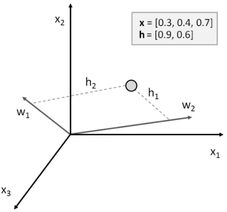
with a data point represented by three original variablesx projected to a two dimensional subspace spanned by w to obtain features h. . 28 2.3 The concept of low-rank + sparse matrix decomposition using an

example “part-worth coefficients” matrix of size 10 x 10 decomposed into two 10 x 10 matrices with low rank or sparse structure. Lighter colors represent larger values of elements in each decomposed matrix. 31 2.4 The concept of the exponential family sparse restricted Boltzmann

machine. The original data are represented by nodes in the visible layer by [x1, x2], while the feature representation of the same data is represented by nodes in the hidden layer [h1, h2, h3, h4]. Undirected edges are restricted to being only between the original layer and the hidden layer, thus enforcing conditional independence between nodes in the same layer. . . 35

(8)

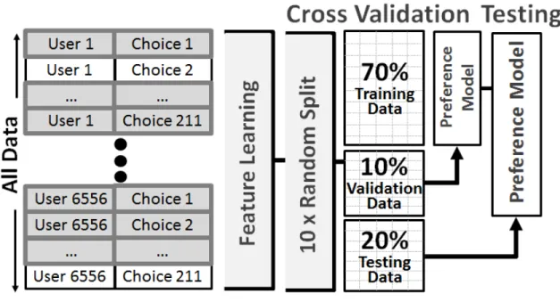
2.5 Data processing, training, validation, and testing flow. . . 45

2.6 Optimal vehicle distribution visualization. Every point represents the optimal vehicle for one consumer. In the left column, the opti-mal vehicle is inferred using the utility model with original variables. In the right column, LSD features are used to infer the optimal ve-hicle. In the first row, the optimal vehicles from SCI-XA customers are marked in big red points. Similarly, the optimal vehicles from MAZDA6, ACURA-TL and INFINM35 customers are marked in big red points respectively. . . 52 3.1 An example of conjoint task with written description of functional

attributes . . . 65 3.2 An example of conjoint task with written description of functional

attributes and aesthetics attributes . . . 66 3.3 An example of conjoint task with written description of functional

attributes and image description of aesthetics attributes . . . 66 3.4 A snapshot of the ranking page in the crowdsourcing web application. 69 3.5 Sorted Aesthetics Values . . . 74

3.6 Top 10 SUVs for each aesthetics attribute levels . . . 75 3.7 The relative importance of attribute in conjoint analysis with images.

The value of relative importance is hidden due to the Intelligence Properties Protection for General Motors . . . 76

3.8 The relative importance of attribute in conjoint analysis with textual description. The value of relative importance is hidden due to the Intelligence Properties Protection for General Motors . . . 77 3.9 The relative importance of attribute in conjoint analysis when

in-cluding brand. The value of relative importance is hidden due to the Intelligence Properties Protection for General Motors . . . 78 4.1 Overview of design process using the proposed quantitative

commu-nication model. The goal is to predict a region of visual attraction, denoted in grey given a particular design. . . 80

4.2 AlexNet convolutional neural network structure. . . 85 4.3 L1 Regression. . . 87

(9)

4.4 Deconvolutional neural network method flow. . . 90 4.5 L1 regression prediction performance for all 10 design attributes with

the x axis representing the vehicle ID and the y axis representing the attribute values and estimated values. . . 92 4.6 Examples of predicted attraction regions for design attribute ’Active’.

The top row corresponds to an unknown design feature describing and ‘Active‘ car, seemingly focused on vehicle headlights, while the bot-tom row corresponds to a sepearte unknown design feature, seemingly focused on the front quarter-panel and door. . . 94 5.1 Overview of the proposed deep learning approach for aesthetic design

appeal prediction for heterogeneous customers. Grey boxes represent the inputs, white boxes represent outputs, and rounded corner boxes represent the model or algorithm. . . 100

5.2 Discriminator and generator in conditional generative adversarial net-work. Grey boxes represent inputs and white boxes represents con-volutional layers in discriminator and upsampling layers. . . 101 5.3 Siamese network of identical conditional generative adversarial

net-works, with conditioning on design and customer labels. This struc-ture is used to model a customer’s aesthetic perceptiony_ijk for a given design attribute. . . 107

5.4 A snapshot of the ranking page in the crowdsourcing web application. 111 5.5 The customer data distribution of (a) Age, (b) Income Level, (c)

Family Size, and (d) Housing/Living Region, where ”Metro” means ”Metropolitan”, ”Sub” means ”Suburban”, ”Town” means ”Small Town”, and ”Farming” means ”Farming Area”. . . 113 5.6 Randomly generated vehicle designs from the cGAN generator. These

images provide evidence the cGAN is capturing the data distribution of vehicles, particularly with more realism than similar approaches by the authors such as variational autoencoders. . . 115

5.7 Visualization of salient design regions for the 2014 Range Rover Sport. The first row shows salient regions for ‘Suburban’ ‘Women,’ while the second row shows salient regions for ‘Rich’ ‘Men’ ’Over 40.” 116

(10)

LIST OF TABLES

Table

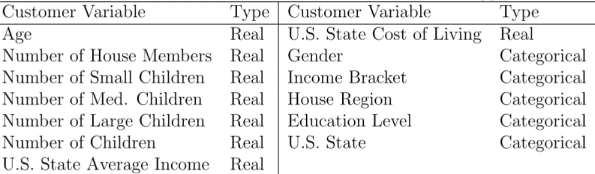
2.1 Customer variables xc and their variable types . . . 24

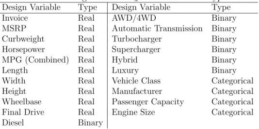
2.2 Design variables xd and their variable types . . . 25

2.3 Averaged preference prediction accuracy on held-out test data using the logit model with the original variables or the three feature rep-resentations. Average and standard deviation were calculated from 10 random training and testing splits common to each method, while test parameters for each method were selected via cross validation on the training set. . . 46

4.1 Description of the four data sets used in this work . . . 83 4.2 Ten design attributes used for partial ranking evaluation for 2D

ve-hicle images. . . 90 5.1 Design labels . . . 110 5.2 Customer labels . . . 110

5.3 Averaged prediction accuracy and its standard deviation on hold-out test data using the Siamese Net with image features, design labels, customer labels or only with the design and customer labels. Average and standard deviation were calculated from 5 random training and testing splits common to each method. . . 117

(11)

ABSTRACT

Creating a form that is attractive to the intended market audience is one of the greatest challenges in product development given the subjective nature of preference and heterogeneous market segments with potentially different product preferences. Accordingly, product designers use a variety of qualitative and quantitative research tools to assess product preferences across market segments, such as design theme clinics, focus groups, customer surveys, and design reviews; however, these tools are still limited due to their dependence on subjective judgment, and being time and resource intensive. In this dissertation, we focus on a key research question: how can we understand and predict more reliably the preference for a future product in heterogeneous markets, so that this understanding can inform designers’ decision-making?

We present a number of data-driven approaches to model product preference. In-stead of depending on any subjective judgment from human, the proposed preference models investigate the mathematical patterns behind users choice and behavior. This allows a more objective translation of customers’ perception and preference into ana-lytical relations that can inform design decision-making. Moreover, these models are scalable in that they have the capacity to analyze large-scale data and model cus-tomer heterogeneity accurately across market segments. In particular, we use feature representation as an intermediate step in our preference model, so that we can not only increase the predictive accuracy of the model but also capture in-depth insight into customers’ preference.

(12)

We tested our data-driven approaches with application in visual aesthetics pref-erence. Our results show that the proposed approaches can obtain an objective mea-surement of aesthetic perception and preference for a given market segment. This measurement enables designers to reliably evaluate and predict the aesthetic appeal of their designs. We also quantify the relative importance of aesthetic attributes when both aesthetic attributes and functional attributes are considered by customers. This quantification has great utility in helping product designers and executives in design reviews and selection of designs. Moreover, we visualize the possible factors affecting customers’ perception of product aesthetics and how these factors differ across differ-ent market segmdiffer-ents. Those visualizations are incredibly important to designers as they relate physical design details to psychological customer reactions.

The main contribution of this dissertation is to present purely data-driven ap-proaches that enable designers to quantify and interpret more reliably the prod-uct preference. Methodological contributions include using modern probabilistic ap-proaches and feature learning algorithms to quantitatively model the design process involving product aesthetics. These novel approaches can not only increase the pre-dictive accuracy but also capture insights to inform design decision-making.

(13)

CHAPTER I

Introduction

1.1

Introduction

Creating a form that is attractive to the intended market audience is one of the greatest challenges in product development. In the early design phase, designers trans-late the needs and desires (e.g. customers need an aesthetically appealing product) to actual design decisions. These decisions are usually defined using design attributes, which are the design properties that the people who will experience the product, namely, the criteria they will use to judge the product (e.g., luxuriousness, ease of use, etc). Design attributes may not be measurable, thus designers need to make a mapping from design attributes to the measurable design characteristics, which are the design properties that the designer can explicitly act upon by manipulating the design (e.g. color, length, shape). To create an attractive product, designers must understand how customers perceive the design of a product; however, this under-standing can be difficult to gain due to the inherent subjectivity of preference and the heterogeneity of customers across market segments. Moreover, designers need to translate such understanding into the language of engineering so that it can inform design decision-making. In other words, designers need to understand which design characteristics can affect preference and how they affect it.

(14)

mak-ing related design decisions; however, this can brmak-ing a large risk in the design process in that such subjective insights may lead to the wrong preference reaction when imple-mented in the actual product. Accordingly, designers often use a variety of qualitative and quantitative methods to assess product preferences, such as design theme clinics, focus groups, customer surveys, and design reviews. While these methods can provide further insights into the rationale for product preference, they are still limited due to two main drawbacks. First, these methods require customers to translate their subjective perception into semantic or numerical assessment, and the designers must then translate the assessment back into an attractive design. Communication errors are likely to occur during this translation process as customers often cannot articu-late accurately why they like or dislike a design (Nisbett and Wilson, 1977; Silvera et al., 2002). Also, designers are often geographically or culturally distant from the potential customers. Second, these methods are not scalable because they are labor and resource intensive. Lack of scalability can be problematic especially for product domains where there are hundreds of market segments. These drawbacks present a research gap in translating customers’ perception and preference into an attractive product in a more predictive and scalable way.

In this dissertation, we focus on a key research question: how can we understand and predict more reliably the aesthetic perception and preference for a future prod-uct in a heterogeneous market, so that this understanding can inform the designers’ decision-making. To answer this question, we propose a number of data-driven ap-proaches to model product preference. Instead of having a human analyst acting as the interpreter of data, the proposed preference models investigate the mathematical patterns behind users’ responses. This allows a more objective translation of cus-tomers’ preference into analytical relations that can inform design decision-making. Moreover, these models are scalable in that they have the capacity to analyze the datasets including a large number of customers and designs and model customer

(15)

heterogeneity accurately across market segments.

In particular, we test our proposed data-driven models with application in visual aesthetics preference. Product aesthetics have long been recognized as a critically important factor for the success of a product. An aesthetically appealing appear-ance not only evokes pleasant emotions but also communicates meaning, quality, and product integrity to the customers before they physically interact with the product. Customers exhibit an involuntary aesthetic reaction and infer the presence of other product attributes based on this aesthetics reaction. One can assume naturally that customers prefer beautiful designs to ugly ones, even in highly functional product domains. Moreover, customers are willing to pay more money for a more beautiful product.

1.2

Research Problem

Aesthetics is a very old concept with root in the Greek wordaisthesis, whose origi-nal meaning can be translated as understanding through sensory perception (Hekkert and Leder, 2008). The definition of aesthetics has slightly changed over time. Nowa-days, aesthetics refers to the pleasure attained from sensory perception (Hekkert, 2006). Sensory input traditionally can be visual, auditory, tactile (somatic), olfac-tory, and gustatory; today we also recognize other sensory input such as motion, tem-perature or pain. Product aesthetics is defined here as the process of how products communicate meaning and evoke emotion through the senses (Khalid and Helander, 2006). The aesthetic reaction can be quick, often representing a first reaction to the product (Reber et al., 2004). In addition, an aesthetic reaction often encompasses an overall assessment of the product. Customers are attracted by the aesthetic appeal of the designed artifact and they tend to relate the function of a product to its aesthetic appeal (Norman, 2005).

(16)

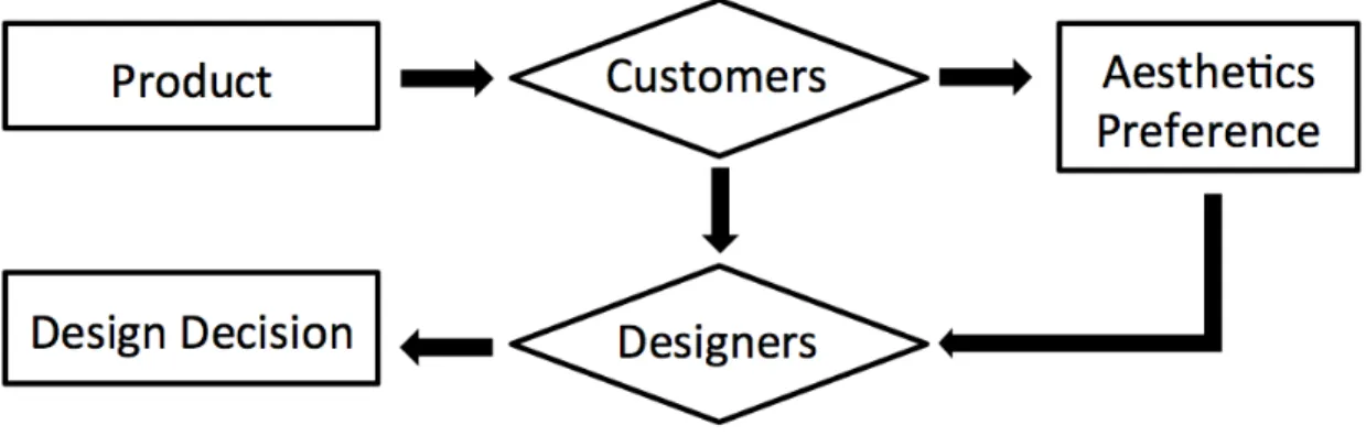
Figure 1.1: A symbolic model for the design process including aesthetic preferences in design decisions

very complex. To study this process, we illustrate the process using a symbolic model, which is an abstract description of the real world giving an approximate rep-resentation of more complex functions of physical systems, in figure 1.1. In this aesthetics preference model, customers are the perceivers of the product aesthetics, who receive the sensory information from the product, resulting in an aesthetics per-ception or preference (adapted from (Leder et al., 2004; Hekkert, 2006)). Designers observe the users choices or behaviors, then infer the underlying aesthetics percep-tion and preference, followed by interpreting the possible factors affecting aesthetics preference, finally, designers refer to this interpretation when making design deci-sions. Moreover, we can use quantitative model to represent this symbolic model by mathematical relations.

In this dissertation, the general research problem is to model the design process including aesthetics preferences quantitatively. The goal of this quantitative model is to extract useful information about product aesthetics more objectively in order to inform design decision-making more reliably. While product aesthetics involve many senses, in this dissertation we focus only on modeling aesthetics related to visual sen-sory perception. From here on, when referring to aesthetics we mean specifically visual aesthetics. This choice is made in part because visual input is dominant in product

(17)

aesthetics (Goldstein and Brockmole, 2016; Hekkert, 2006). While the methodology we present may be applicable to other sensory input, this generalization is beyond the scope of the dissertation.

Within the general research problem above we extract and address four specific research questions:

1. Does the product achieve the desired aesthetic design attributes for a given market segment?

2. How important are the aesthetic design attributes when compared with func-tional attributes and price?

3. What are the possible factors affecting customers’ perception of product aes-thetic appeal?

4. How do these factors differ across different market segments?

1.3

Aesthetics Preference Models

To address the research questions we develop data-driven aesthetics preference models that can map the visual information to the customers’ aesthetic perception and preference. We then investigate the interpretation of this mapping in order to understand what are the factors that account for the observed emotional responses. Finally, we examine how we can apply the findings to support the decision-making process of practicing designers.

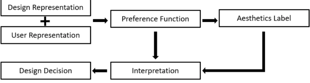
A model-based quantitative process for including aesthetic preferences in design decision making typically consists of five steps: design and user representation, prefer-ence function model, aesthetics labeling, interpretation, and design decision as shown in Figure 1.2. The first step, serving as input to the preference function model, is a mathematical representation of the design. This input is different from that in a

(18)

Figure 1.2: A model-based process to account for aesthetic preferences in design de-cisions

design optimization model, which classifies the input into design variables that are quantities specifying different states of a system by assuming different values and design parameters that are quantities that are given one specific value in any particu-lar model statement. The input design representation includes all measurable design quantities that believed to be predictive to product aesthetics. This representation can include design variables (as shown in Chap II), design parameters (as shown in Chap V), design characteristics (as shown in Chap II and III), and measurable de-sign attributes (as shown in Chap III). In addition, dede-sign representation can also be non-parametric, for example, the design images (as shown in Chap IV and V). A representation of the customers may also be included as part of the model input espe-cially when heterogeneous markets are considered (as shown in Chap II and V). We denote the design representation as Xd and the customer representation as Xc. The

second step is the creation of the preference function which can predict the customer preference for the third step of the model, the aesthetics preference. This preference function, denoted as f, can implicitly capture the aesthetics preference by predict-ing subsequent user behaviors or user choices. Specifically, we want to estimate the preference function, so that y = f(Xd,Xc), where aesthetics labels, denoted as y,

are the quantities resulting from users potential aesthetics preferences, such as users choices (e.g. Chap III), crowdsourced responses (e.g. Chap IV), and users behavior

(19)

(e.g. Chap V). The fourth step is interpretation, where the preference relation is quantitatively analyzed through mathematical tools and visualization. For example, we can determine the optimal design by maximizing the preference as shown in Chap II, investigate the influence of visual sensory by control experiments as shown in Chap III, approximately inverse the preference function as shown in Chap IV, and visualize the salient design regions as shown in Chap V. Those tools play the same role as

designers in the symbolic model. Finally, design decisions are made based on the results of this analysis.

There are three challenges in aesthetics preference modeling. The first challenge is to determine an appropriate mathematical representation of the design and its cus-tomers in the model. The explicit mathematical representations used in quantitative preference model are usually a set of mathematical elements, which are supposed to contain influential information in aesthetics phenomena. Unlike other types of prefer-ence, aesthetics preference is dominantly evoked by visual inputs. The visual sensory information is best preserved in the form of an image or video, which are not the conventional modalities of input data in a quantitative model. As a result, we need to transform this visual information into an explicit representation that can be used in a quantitative model.

The second challenge is how to handle the complexity of the nonlinear mapping between the design representation and the aesthetics labels. In the product design community, linear logit functions have been widely used in preference modeling, be-cause the logit function is easy to compose and to interpret, and it has a solid the-oretical foundation for model diagnostics under known assumptions; however, the assumptions behind the logit function, such as linearity and independence, may not be appropriate in most real design situations. As a result, conclusions from these models maybe inaccurate or inappropriate. The predictive accuracy of linear logit models may be low especially in scenarios where the preference relationship is highly

(20)

nonlinear.

Sophisticated nonlinear models have been developed to model this process with high accuracy, such as content-based collaborative filtering (Pazzani and Billsus, 2007), kernel methods (Ren et al., 2013), and Bayesian approach (Srivastava and Schrater, 2012); however, these bring the third challenge for aesthetic preference mod-eling. With the nonlinear models, predictive performance is significantly improved at the cost of reduced interpretability. In contrast, with the linear models, interpretabil-ity is often possible but predictive power is relatively poor due to assumptions that typically do not hold, namely, linearity (Bodenhofer and Klawonn, 2004), feature in-dependence (Holt, 1986;Torrance et al., 1995), homogeneity (Birol et al., 2006;Feick and Higie, 1992), and complex noise distributions (Althaus, 2003). Subsequently, we must face the trade-off between interpretability and predictive accuracy or develop new approaches to interpret nonlinear functions.

1.4

Related Work

1.4.1 Aesthetics Research

Research in aesthetics can be generally classified into two categories: descriptive study and quantitative study. In a descriptive study, design researchers or practicing designers play the role of the preference function and interpretation in the aesthet-ics preference model. They link the products and customers with the aesthetics preference through their observation and then translate the observation into design principles. The descriptive study of aesthetics dates back to centuries ago, for exam-ple, the use of the golden ratio. In recent decades, much of descriptive study research focused on finding properties of objects and simple patterns that determine aesthetic preference.

(21)

organizational and meaningful properties (see (Hekkert, 1995) for an overview). The psychophysical properties refer to the product properties that can be quantified, such as size and color. These properties affect aesthetics preference relationally and con-textually. For example, it has been demonstrated that hues are preferred in the order blue, green or red, and yellow (McManus et al., 1981). The organizational properties focus on how our visual system organizes information by analyzing edges, contours, blobs, and basic geometrical shapes. Gestalt psychology is a well-known organiza-tional property, which studies the relationship between elements and the whole. There are several principles in Gestalt psychology; for example, the principle of similarity

demonstrates that elements that look similar in shape, color, or size, are likely seen as belonging together. Meaningful properties are the subjective properties that are determined based on one’s knowledge, culture, and previous experiences. A pioneer-ing study in this category is ‘familiarity breeds likpioneer-ing’ (Zajonc, 1968), which suggests that people may prefer a familiar design solution. Descriptive research in aesthetics has provided some valuable principles. While these principles have been successfully employed in practice, there is still a need for more detailed studies in aesthetics due to the heterogeneity of aesthetics perception. This need is further exacerbated for customer-centered products.

Quantitative research in aesthetics allows designers to investigate aesthetics from a much closer distance. Rather than having the human as the interpreter, quantita-tive studies in aesthetics aim at investigating the mathematical relationship between design, customer, and aesthetic preference. A common approach is to first decompose a complex form into design characteristics. For example, the form of an automobile can be broken into headlight, grill, etc. This decomposition process is also called atomization (Durgee, 1988). After atomizing the form, how design characteristics affect aesthetics preference can be determined either separately or jointly. (Orsborn et al., 2009) shows an example of quantifying aesthetic preference in a utility function

(22)

via atomization. While designers can mathematically represent the form of design through atomization, this approach is still limited as the visual sensory information is not well preserved. Moreover, the three challenges discussed previously remain to be solved.

1.4.2 Feature Learning

Feature learning is a research field that has been applied to improve the repre-sentation of input data in various applications. Feature learning methods transform the original data representation into a feature representation, which can be effectively exploited in the predictive modeling task. The feature representation consists of fea-tures which are functions of the design variables in the original design representation, for example, a nonlinear combination of the geometric variables, the mean value of a set of pixel values, or the design variable itself.

There is a long history of using features to represent designs in the design com-munity. These design features may be manually defined by designers based on an obvious interpretation or classification of the features, such as a set of parametric handles to manipulate vehicle silhouettes (Petiot and Dagher, 2011; Poirson et al., 2013; Reid et al., 2013; Ren et al., 2013). Using finite shape grammars to form more complex representations is another type of design representation (McCormack et al., 2004;Orsborn et al., 2006; Pugliese and Cagan, 2002). Hybrid approaches that learn the set of handles have been studied, for example, autoencoders for 3D object ma-nipulation to affect attribute ratings (Yumer et al., 2015), and representations that combine hand-crafted and implicitly learned representations to capture design free-dom and brand recognition (Burnap et al., 2016a).

In addition to the design-specific features, there is a vast amount of work from computer vision researchers on features automatically learned from the data. These features are more general for a variety of tasks and have achieved great success such as

(23)

object recognition(Krizhevsky et al., 2012), speech recognition (Hinton et al., 2012), and natural language process (Collobert and Weston, 2008). In this context features are more abstract data-derived mathematical constructs and may not have imme-diate or obvious interpretation. The feature learning methods can be divided into two categories: supervised feature learning and unsupervised feature learning. Su-pervised feature learning means learning features from labeled data, such as neural networks (Krizhevsky et al., 2012) and supervised dictionary learning (Mairal et al., 2009). These feature learning functions may be generalized to the task outside of the training data set (Gatys et al., 2015; Karayev et al., 2013). Unsupervised fea-ture learning means learning feafea-tures from unlabeled data, such as sparse coding (Lee et al., 2006), deep autoencoders (Kingma and Welling, 2013), and deep Boltz-mann machine(Salakhutdinov and Hinton, 2009). These feature learning methods are promising for use in aesthetics preference modeling.

1.4.3 Preference Learning

Preference is also an important topic in the machine learning field. The research related to this topic is often referred to as preference learning. In general, the goal of preference learning is to construct (“learn”) a predictive preference model from observed preference data. Specifically, there is a training set, which is a set of samples whose preferences are known. A preference learning task is to learn a function from the training set that predicts preferences for a new set of samples. Preference learning is often viewed as a supervised learning task, whose training samples are pairs consisting of an input object (also called independent variable in statistics) and an associated output label (also called dependent variable in statistics).

There is an overlap between preference learning and aesthetics preference model-ing, as both of approaches aim at constructing the functions linking the input product representation and its preference label using data. Despite this commonality, there

(24)

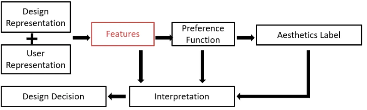
Figure 1.3: The proposed aesthetics preference model

are several differences distinguishing preference learning from aesthetics preference modeling. Although a predictive preference function is an important component of an aesthetics preference model, the primary goal of the model is to inform design de-cision making. To achieve this goal, the model must be interpretable to enhance the designers’ understanding of the targeted users. Preference learning primarily empha-sizes the use of the preference function, which is usually highly nonlinear, to predict future user choices, and understanding of why the choices are made is of secondary interest. As a result, preference learning may have high predictive accuracy, but low interpretability. This difference prevent designers from directly employing preference learning model to inform design decision making.

1.4.4 Proposed Approach

In this dissertation, we propose to use the feature learning method as an interme-diate step between the original design representation and aesthetics labeling as shown in Figure 1.3. The idea of modeling preference via feature learning is motivated by the success of using feature learning to improve prediction accuracy in various appli-cations (Girshick et al., 2014; Guyon and Elisseeff, 2003; Li et al., 2010; Mittelman et al., 2013). Moreover, research in the design community has shown that consumers prefer to perceive a product through the high-level design attributes such as compact

(25)

design, which cannot be directly controlled by the designers, instead of the original design characteristics or variables such as “the length is 10 cm”, which can be directly controlled by designers. Feature learning may help designers to discover rules for how to change the perceived design attributes by changing the design characteristics or variables accordingly.

Aesthetic preference modeling can benefit from using feature representation in several ways. First, feature learning can transform multimodal data into a unified representation so that the preference model can relate information in different data modalities together to infer preference. Second, previous research has shown that transforming data variables into more easily human-memory ”chunked” perceptual features justifies the linear models commonly used in the design community ( Living-stone and Hubel, 1987). Classic classification models, such as the l2 regularized logit model, may have superior prediction accuracy with features as the model variables rather than with the original variables as shown in (Burnap et al., 2014). Third, instead of directly interpreting the highly nonlinear aesthetic preference function, it may be easier to interpret a preference mapping with the feature representation as an intermediate stage, because the interpretation process can be decomposed into two steps: interpreting the features and interpreting the less complex preference function. These issues are explored in more detail in the later chapters of the dissertation.

1.5

Dissertation Contribution

The main contribution of this dissertation is to demonstrate that we can quantify product preference using a purely data-driven approach in a way that has value for the practicing designer. We aim to provide designers a method to more objectively measure the product preference. In addition, we aim to develop a number of quantita-tive models that interpret how portions of the design space affect product perception and preference in both homogeneous and heterogeneous markets. Moreover, these

(26)

models are scalable to hundreds or thousands of markets, an important consideration for enterprises engaged in product design across globally dispersed markets.

Methodological contributions include introducing feature representation as an in-termediate step in preference modeling. Dissertation results show that there is an increase of preference prediction accuracy when using feature learning methods, as compared with the original data representation. These results also suggest features indeed represent better the customers underlying design preferences, thus offering deeper insights to inform design decisions. Furthermore, the dissertation addresses how to deal with multimodal data forms, and demonstrates training models using large-scale multimodal data including 2D images, numerical labels, and crowdsourced response data.

1.6

Dissertation Overview

The rest of the dissertation is organized as follows: Chapter 2 presents a product preference model which uses feature representation as an intermediate step between design representation and preference function. This model is applied to predict au-tomobile purchase decisions. The results show that the use of features offers im-provement in prediction accuracy, and the interpretation and visualization of these feature representations can be used to support data-driven design decisions. More-over, a theoretical error bound is given to guarantee the model fitness. Chapter 3 presents a novel approach to quantify more objectively aesthetic attributes as well as their relative importance vs. other attributes. Specifically, this approach provides designers quantitative evidence to evaluate whether a design concept achieves the desired aesthetic design attributes; it further investigates the relative importance of aesthetic attributes when compared with functional attributes and price. These find-ings offer deeper insights on how customers make trade-off between product aesthetics and function. Chapter 4 presents a data-driven method building on features from a

(27)

deep convolutional neural network. This data-driven method can predict aesthetic attribute values for given design images. Importantly, this model can identify visual attention regions that affect customers’ aesthetics perception. Chapter 5 presents a scalable deep learning approach that predicts how customers across different mar-ket segments perceive aesthetic designs, and provides a visualization to aid product design. Chapter 6 gives a summary of results, contributions, and future directions.

(28)

CHAPTER II

Improving Design Preference Prediction Accuracy

with Feature Learning

2.1

Introduction

In this chapter we explore how we can introduce features to improve preference prediction accuracy while being able to extract insights for design decisions. Much research has been devoted to develop design preference models that predict customer design choices. A common approach is to: (i) collect a large database of previous pur-chases that includes customer data, e.g., age, gender, income, and purchased product design data, e.g., number of cylinders, length, curb weight — for an automobile; and (ii) statistically infer a design preference model that links customer and product vari-ables, using conjoint analysis or discrete choice analysis such as logit, mixed logit, and nested logit models (Berkovec and Rust, 1985;McFadden and Train, 2000).

However, a customer may not purchase a vehicle solely due to interactions be-tween these two sets of variables, e.g., a 50-year old male prefers 6-cylinder engines. Instead, a customer may purchase a product for more ‘meaningful’ design attributes that are functions of the original variables, such as environmental sustainability or sportiness (Reid et al., 2012; Norman, 2005). These meaningful intermediate func-tions of the original variables, both of the customer and of the design, are hereafter

(29)

termed features. We posit that using customer and product features, instead of just the original customer and product variables, may increase the prediction accuracy of the design preference model.

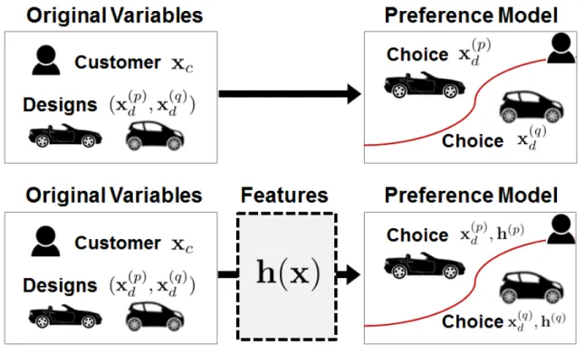
Our goal then is to find features that improve this preference prediction accuracy. To this end, one common approach is to ask design and marketing domain experts to choose these features intuitively, such as a design’s social context (He et al., 2014) and visual design interactions (Sylcott et al., 2013). For example, eco-friendly vehicles may be a function of miles per gallon (MPG) and emissions, whereas environmen-tally active customers may be a function of age, income, and geographic region. An alternative explored in this chapter is to find features ‘automatically’ using feature learning methods studied in computer science and statistics. As shown in Figure 2.1, feature learning methods create an intermediate step between the original data and the design preference model by forming a more efficient “feature representation” of the original data. Certain well-known methods such as principal component analysis may be viewed similarly, but more recent feature learning methods have shown im-pressive results in 1D waveform prediction (Hinton et al., 2012) and 2D image object recognition (Krizhevsky et al., 2012).

We conduct an experiment on automobile purchasing preferences to assess whether three feature learning methods increase design preference prediction accuracy: (1) principle component analysis, (2) low-rank + sparse matrix decomposition, and (3) exponential family sparse restricted Boltzmann machines (Salakhutdinov et al., 2007). We cast preference prediction as a binary classification task by asking the question, “given customerx, do they purchase vehiclepor vehicleq.” Our data set is comprised of 1,161,056 data points generated from 5582 real passenger vehicle purchases in the United States during model year 2006 (MY2006).

The first contribution of this work is an increase of preference prediction accuracy by 2%-7% just using simple “single-layer” feature learning methods, as compared

(30)

Figure 2.1: The concept of feature learning as an intermediate mapping between vari-ables and a preference model. The diagram on top depicts conventional design preference modeling (e.g., conjoint analysis) where an inferred pref-erence model discriminates between alternative design choices for a given customer. The diagram on bottom depicts the use of features as an in-termediate modeling task.

(31)

with the original data representation. These results suggest features indeed better represent the customer’s underlying design preferences, thus offering deeper insight to inform decisions during the design process. Moreover, this finding is complementary to recent work in crowdsourced data gathering (Burnap et al., 2015; Panchal, 2015) and nonlinear preference modeling (Chapelle and Harchaoui, 2004; Evgeniou et al., 2007)) since they do not affect the preference model or data set itself.

The second contribution of this work is to show how features may be used in the design process. We show that feature interpretation and feature visualization offer designers additional tools for augmenting design decisions. First, we interpret the most influential pairings of vehicle features and customer features to the preference task, and contrast this with the same analysis using the original variable represen-tation. Second, we visualize the theoretically optimal vehicle for a given customer within the learned feature representation, and show how this optimal vehicle, which does not exist, may be used to suggest design improvements upon current models of vehicles that do exist in the market.

Methodological contributions include being the first to use recent feature learn-ing methods on heterogeneous design and marketlearn-ing data. Recent feature learnlearn-ing research has focused on homogeneous data, in which all variables are real-valued num-bers such as pixel values for image recognition (Krizhevsky et al., 2012; Lee et al., 2011); in contrast, we explicitly model the heterogeneous distribution of the input variables, for example ‘age’ being a real-valued variable and ‘General Motors’ being a categorical variable. Subsequently, we give a number of theoretical extensions: First, we use exponential family generalizations for the sparse restricted Boltzmann ma-chines, enabling explicit modeling of statistical distributions for heterogeneous data. Second, we derive theoretical bounds on the reconstruction error of the low-rank + sparse matrix decomposition feature learning method.

(32)

to increase prediction accuracy by the design community, as well as feature learning advances in the machine learning community. Section 2.3 sets up the preference prediction task as a binary classification problem. Section 2.4 details three feature learning methods and their extension to suit heterogeneous design and market data. Section 2.6 details the experimental setup of the preference prediction task, followed by results showing improvement of preference prediction accuracy. Section 2.5 proves the theoretical bounds on the reconstruction error of the low-rank + sparse matrix decomposition feature learning methods. Section 2.7 details how features may be used to inform design decisions through feature interpretation and feature visualization. Section 2.8 summarizes the chapter.

2.2

Background and Related Work

Design preference modeling has been investigated in design for market systems, where quantitative engineering and marketing models are linked to improve enterprise-wide decision making (Wassenaar and Chen, 2003;Lewis et al., 2006;Michalek et al., 2005). In such frameworks, the design preference model is used to aggregate input across multiple stakeholders, with special importance on the eventual customer within the targeted market segment (Chen et al., 2013).

These design preference models have been shown to be especially useful for the design of passenger vehicles, as demonstrated across a variety of applications such as engine design (Wassenaar et al., 2005), vehicle packaging (Kumar et al., 2007), brand recognition (Burnap et al., 2016a), and vehicle styling (Orsborn et al., 2009;

Reid et al., 2012;Sylcott et al., 2013). Connecting many of these research efforts is the desire for improved prediction accuracy of the underlying design preference model. With increased prediction accuracy, measured using “held out” portions of the data, greater confidence may be placed in the fidelity of the resulting design conclusions.

(33)

sta-tistical models to capture the heterogeneous and stochastic nature of customer pref-erences; examples yuinclude mixed and nested logit models (McFadden and Train, 2000;Berkovec and Rust, 1985), consideration sets (Morrow et al., 2014), and kernel-based methods (Chapelle and Harchaoui, 2004; Evgeniou et al., 2007; Ren et al., 2013); and (ii) creating adaptive questionnaires to obtain stated information more efficiently using a variety of active learning methods (Toubia et al., 2003; Abernethy et al., 2008).

This work is different from (i) above in that the set of features learned is agnostic of the particular preference model used. One can just as easily switch out thel2 _logit design preference model used in this paper for another model, whether it be mixed logit or a kernel machine. This work is also different from (ii) in that we are working with a set of revealed data on actual vehicle purchases, rather than eliciting this data through a survey. Accordingly, this work is among recent efforts towards data-driven approaches in design (Tuarob and Tucker, 2015), including design analytics (Van Horn and Lewis, 2015) and design informatics (Dym et al., 2005), in that we are directly using data to augment existing modeling techniques and ultimately suggest actionable design decisions.

2.2.1 Feature learning

Feature learning methods capture statistical dependencies implicit in the original variables by “encoding” the original variables in a new feature representation. This representation keeps the number of data the same while changing the length of each data point from M variables to K features. The idea is to minimize an objective function defining the reconstruction error between the original variables and their new feature representation. If this representation is more meaningful for the discriminative design preference prediction task, we can use the same supervised model (e.g., logit model) as before to achieve higher predictive performance. More details are given in

(34)

Section 2.4.

The first feature learning method we examined is principal component analysis (PCA). While not conventionally referred to as a feature learning method, PCA is chosen for its ubiquitous use and its qualitative difference from the other two methods. In particular, PCA makes the strong assumption that the data is Gaussian noise distributed around a linear subspace of the original variables, with the goal of learning the eigenvectors spanning this subspace (Friedman et al., 2001). The features in our case are the coefficients of the original variables when projected onto this subspace or, equivalently, the inner product with the learned eigenvectors.

The second feature learning method is low-rank + sparse matrix decomposition (LSD). This method is chosen as it defines the features implicitly withing the prefer-ence model. In particular, LSD decomposes the “part-worth” coefficients contained in the design preference model (e.g., conjoint analysis or discrete choice analysis) into a low-rank matrix plus a sparse matrix. This additive decomposition is motivated by results from the marketing literature suggesting certain purchase consideration are linearly additive (Gonzalez and Wu, 1999), and thus well captured by decomposed matrices (Evgeniou et al., 2005). An additional motivation for a linear decomposition model is the desire for interpretability (Hauser and Rao, 2004). Predictive consumer marketing oftentimes uses these learned coefficients to work hand-in-hand with engi-neering design to generate competitive products or services (Papalambros and Wilde, 2000). Such advantages are bolstered by separation of factors captured by matrix de-composition, as separation may lead to better capture of heterogeneity among market segments (Lenk et al., 1996). Readers are referred to (Netzer et al., 2008) for further in-depth discussion.

The third feature learning method is the exponential family sparse restricted Boltzmann machine (RBM) (Smolensky, 1986;Lee et al., 2008). This method is cho-sen as it explicitly reprecho-sents the features, in contrast with the LSD. The method is a

(35)

special case of a Boltzmann machine, an undirected graph model in which the energy associated within an energy state space defines the probability of finding the system in that state (Smolensky, 1986). In the RBM, each state is determined by both visible and hidden nodes, where each node corresponds to a random variable. The visible nodes are the original variables, while the hidden nodes are the feature representa-tion. The “restricted” portion of the RBM refers to the restriction on visible-visible connections and hidden-hidden connections, later detailed and depicted in in Section 2.4 and Figure 2.4, respectively.

All three feature learning methods are considered “simple” in that they are single-layer models. The aforementioned results in 1D waveform speech recognition and 2D image object recognition have been achieved using hierarchical models, built by stacking multiple single-layer models. We chose single-layer feature learning methods here as an initial effort and to explore parameter settings more easily; as earlier noted, there is limited work on feature learning methods for heterogeneous data (e.g., categorical variables) and most advances are currently only on homogeneous data (e.g., real-valued 2D image pixels).

2.3

Preference Prediction as Binary Classification

We cast the task of predicting a customer’s design preferences as a binary classifi-cation problem: Given customerj, represented by a vector of heterogeneous customer variablesx(cj), as well as two passenger vehicle designs p andq, each represented by a

vector of heterogeneous vehicle design variablesx(_dp) andx(_dq), which passenger vehicle will the customer purchase? We use a real data set of customers and their passenger vehicle purchase decisions as detailed below (Maritz Research Inc., 2007).

(36)

Table 2.1: Customer variables xc and their variable types

Customer Variable Type Customer Variable Type

Age Real U.S. State Cost of Living Real

Number of House Members Real Gender Categorical Number of Small Children Real Income Bracket Categorical Number of Med. Children Real House Region Categorical Number of Large Children Real Education Level Categorical

Number of Children Real U.S. State Categorical

U.S. State Average Income Real

2.3.1 Customer and vehicle purchase data from 2006

The data used in this work combines the Maritz vehicle purchase survey from 2006 (Maritz Research Inc., 2007), the Chrome vehicle variable database (Chrome Systems Inc., 2008), and the 2006 estimated U.S. state income and living cost data from the U.S. Census Bureau (United States Census Bureau, 2006) to create a data set with both customer and passenger vehicle variables. These combined data result in a matrix of purchase records, with each row corresponding to a separate customer and purchased vehicle pair, and each column corresponding to a variable describing the customer (e.g., age, gender, income) or the purchased vehicle (e.g., # cylinders, length, curbweight).

From this original data set, we focus only on the customer group who bought pas-senger vehicles of size classes between mini-compact and large vehicles, thus excluding data for station wagons, trucks, minivans, and utility vehicles. In addition, purchase data for customers who did not consider other vehicles before their purchases were removed, as well data for customers who purchased vehicles for another party.

The resulting database contained 209 unique passenger vehicle models bought by 5582 unique customers. The full list of customer variables and passenger vehicle variables can be found in Tables 2.1 and 2.2. The variables in these tables are grouped into three unit types: Real, binary, and categorical, based on the nature of the variables.

(37)

Table 2.2: Design variables xd and their variable types

Design Variable Type Design Variable Type

Invoice Real AWD/4WD Binary

MSRP Real Automatic Transmission Binary

Curbweight Real Turbocharger Binary

Horsepower Real Supercharger Binary

MPG (Combined) Real Hybrid Binary

Length Real Luxury Binary

Width Real Vehicle Class Categorical

Height Real Manufacturer Categorical

Wheelbase Real Passenger Capacity Categorical

Final Drive Real Engine Size Categorical

Diesel Binary

2.3.2 Choice set training, validation, and testing split

We converted the data set of 5582 passenger vehicle purchases into a binary choice set by generating all pairwise comparisons between the purchased vehicle and the other 208 vehicles in the data set for all 5582 customers. This resulted in N = 1,161,056 data points, where each datum indexed by n consisted of a triplet (j, p, q) of a customer indexed byj and two passenger vehicles indexed bypand q, as well as a corresponding indicator variable y(n) ∈ {0,1} describing which of the two vehicles was purchased.

This full data were then randomly shuffled, and split into training, validation, and testing sets. As previous studies have shown the impact on prediction performance given different generations of choice sets (Shocker et al., 1991), we created 10 random shufflings and subsequent data splits of our data set, and run the design preference prediction experimental procedure of Section 2.6 on each one independently. This work is therefore complementary to studies on developing appropriate choice set gen-eration schemes such as (Wang and Chen, 2015). Full details into the data processing procedure are given in Section 2.6.

(38)

2.3.3 Bilinear design preference utility

We adopt the conventions of utility theory for the measure of customer preference over a given product (Von Neumann and Morgenstern, 2007). Formally, each data point consists of a pairwise comparison between vehiclespandq for customerj , with corresponding customer variables x(cj) for j ∈ {1, . . . ,5582} and original variables of

the two vehicle designs, x(_dp) and x_d(q) for p, q ∈ {1, . . . ,209}. We assume a bilinear utility model for customer j and vehicle p:

Ujp = vecx(_cj)⊗x(_dp) T ,x(_dp) T ω, (2.1)

where ⊗ is an outer product for vectors, vec (·) is vectorization of a matrix, [·,·] is concatenation of vectors, and ω is the part-worth vector.

2.3.4 Design preference model

The preference model refers to the assumed relationship between the bilinear utility model described in Section 2.3.3 and a label indicating which of the two vehicles the customer actually purchased. While the choice of preference model is not the focus of this paper, we pilot-tested popularly used models including l1 and l2 logit model, na¨ıve Bayes,l1 andl2 linear as well as kernelized support vector machine, and random forests.

Based on these pilot results, we chose thel2_{logit model due to its widespread use in} the design and marketing communities (Netzer et al., 2008;Fuge, 2015); in particular, we used the primal form of the logit model. Equation (2.2) captures how the logit model describes the probabilistic relationship between customer j’s preference for either vehiclepor vehicleqas a function of their associated utilities given by Equation (2.1). Note that are Gumbel-distributed random variables accounting for noise over the underlying utility of the customer j’s preference for either vehicle p or vehicle q.

(39)

P(n)=P(j,p,q) =P (Ujp+jp> Ujq+jq) =

eUjp

eUjp₊_eUjq (2.2)

Parameter Estimation

We estimate the parameters of the logit model in Eq. (2.2) using conventional convex loss function minimization using the log-loss regularized with the l2 norm.

min ω,α 1 N N X n=1 (y(n)logP(n)+ (1−y(n)) log(1−P(n))) +αkωk2 (2.3)

wherey(n)=y(jpq)is 1 if customerj chose vehiclepto purchase, and 0 if vehicleqwas purchased; andαis thel2 regularization hyperparameter. The optimization algorithm used to minimize this regularized loss function was stochastic gradient descent, with details of hyperparameter settings given in Section 2.6.

2.4

Feature Learning

We present three qualitatively different feature learning methods as introduced in Section 2.2: (1) principal component analysis, (2) low-rank + sparse matrix decompo-sition, and (3) exponential family sparse restricted Boltzmann machine. Furthermore, we discuss their extensions to better suit the market data described in Section 2.3, as well as derivation of theoretical guarantees.

2.4.1 Principal Component Analysis

Principal component analysis (PCA) maps the original data representation x = [x1, x2, . . . , xM]T ∈ RM×1 to a new feature representation h = [h1, h2, . . . , hK]T ∈ RK×1, K ≤ M, with an orthogonal transformation W ∈ RM×K. Assume that the

original data representationxhas zero empirical mean (otherwise we simply subtract the empirical mean from x). The mapping is given by:

(40)

Figure 2.2: The concept of principle component analysis shown using an example with a data point represented by three original variablesxprojected to a two dimensional subspace spanned by wto obtain features h.

(41)

h=xTW (2.4)

The PCA representation has the following properties: (1) h1 has the largest vari-ance, and the variance of hi is not smaller than the variance of hj for all j < i;

(2) the columns of W are orthogonal unit vectors; and (3) h and W minimize the reconstruction error :

=||x−h||2 (2.5)

When the q columns of W consist of the first q eigenvectors of xTx, the above properties are all satisfied, and the PCA feature representation can be calculated by Equation (2.4). Since PCA is a projection onto a subspace, the features h in this case are not “higher order” functions of the original variables, but rather a linear mapping from original variables to a strictly smaller number of linear coefficients over the eigenvectors.

2.4.2 Low-Rank + Sparse Matrix Decomposition

The utility model Urp given in Equation (2.1) can be rewritten into matrix form,

in which Ω is a matrix reshaped from the “part-worth” coefficients vectorω:

Urp = [ x(cj) T

,1]Ωxp_d (2.6)

The decomposition of the original part-worth coefficients into a low-rank matrix and a sparse matrix may better represent customer purchase decisions than the large coefficient matrix of all pairwise interactions given in Equation (2.1) and as detailed in Section 2.2. Accordingly, we decompose Ω into a low-rank matrix L of rank r

superimposed with a sparse matrix S, i.e. Ω = L+S. This problem may be solved in the general case exactly with the following optimization problem:

(42)

min

L,S l(L,S;Xc,Xd,y) (2.7)

s.t. rank(L)≤r

S∈ C

where Xu and Xc are the full set of customer and vehicle data, y is the vector

of whether customer j chose vehicle p or vehicle q, l(·) is the log-loss without the l2 norm, l(L,S;Xc,Xd,y) = 1 N N X n=1 (y(n)logP(n)+ (1−y(n)) log(1−P(n))) (2.8)

and C is a convex set corresponding to the sparse matrix S. As this problem is intractable (NP-hard), we instead learn this decomposition of matrices using an ap-proximation obtained via regularized loss function minimization:

min

L,S l(L,S;Xc,Xd,y) +λ1||L||∗ +λ2||S||1 (2.9) where||·||∗ is the nuclear norm to promote low-rank structure, and||·||1is thel1-norm. In particular, while a number of low-rank regularizations may be used to solve Eq. (2.9), e.g., trace norm and log-determinant norm (Fazel, 2002). We choose the nuclear norm as it may be applied to any general matrix, while the trace norm and log-determinant regularization are limited to positive semidefinite matrices. More-over, the nuclear norm is often considered optimal as ||L||∗ is the convex envelop of

(43)

Figure 2.3: The concept of low-rank + sparse matrix decomposition using an example “part-worth coefficients” matrix of size 10 x 10 decomposed into two 10 x 10 matrices with low rank or sparse structure. Lighter colors represent larger values of elements in each decomposed matrix.

(Fazel, 2002).

Definition II.1. For matrixL,the nuclear norm is defined as,

||L||∗ :=

min(dim(L))

X

i=1

si(L)

where si(L) is a singular value of L.

2.4.2.1 Parameter Estimation

The non-differentiability of the convex low-rank + sparse approximation given in Eq. (2.9) necessitates optimizations techniques such as augmented Lagrangian (Tomioka et al., 2010), semi-definite programming (Liu and Yan, 2014), and proximal methods (Parikh and Boyd, 2013). Due to theoretical guarantees on convergence, we choose to train our model using proximal methods which are defined as follows.

Definition II.2. Let f :_Rn _→

(44)

Algorithm 1Low-Rank + Sparse Matrix Decomposition Input: Data Xc, Xd, y InitializeL0 ₌₀_,_S0 ₌₀ repeat Lt+1 =proxf(Lt−ηt∇Ltl(L,S;Xc,Xd,y)) St+1 ₌_prox S(St−ηt∇Stl(L,S;X_c,X_d,y)) until Lt_, _St i are converged

proximal operator of f is defined as

prox_f(v) = arg min x f(x) + 1 2||v−x|| 2 2

With these preliminaries, we now detail the proximal gradient algorithm used to solve Eq. 2.9 using low-rank and l1 proximal operators. Denote f(·) =λ1|| · ||∗, and

its proximal operator as proxf. Similarly denote the proximal operator for the l1

regularization term by proxS, i = 1, . . . n. Details of calculating proxf and proxS is

given in the separate Section 2.5 below to maintain continuity of the exposition here.. With this notation, the proximal optimization algorithm to solve Equation (2.9) is given by Algorithm 1. Moreover, this algorithm is guaranteed to converge with constant step size as given by the following lemma (Parikh and Boyd, 2013).

Lemma II.3. Convergence Property

When ∇l is Lipschitz continuous with constant ρ, this method can be shown to con-verge with rate O(_k1) when a fixed step size ηt = η ∈ (0,1/ρ] is used. If ρ is not

known, the step sizes ηt can be found by a line search; that is, their values are chosen

in each step.

2.4.2.2 Error Bound on Low-Rank + Sparse Estimation

We additionally prove a variational bound that guarantees this parameter esti-mation method converges to a unique solution with bounded error as given by the following theorem.

(45)

Theorem II.4. Error Bound on Low-Rank+Sparse Estimation

|4l| ≤λ1min (dim(L0))||L∗−L0||2

where L∗ is the optima of problem (2.9) and L0 is the matrix minimizing the loss

function l(·).

The proof of this theorem is given in Section 2.5.

2.4.3 Restricted Boltzmann machine

The restricted Boltzmann machine (RBM) is an energy-based model in which an energy state is defined by a layer of M visible nodes corresponding to the original variables x and a layer of K features denoted as h. The energy for a given pair of original variables and features determines the probability associated with finding the system in that state; like nature, systems tend to states that minimize their energy and thus maximize their probability. Accordingly, maximizing the likelihood of the observed data x(1). . .x(N) ∈ _RM _{and its corresponding feature representation} h(1). . .h(N) ∈ _RK _{is a matter of finding the set of parameters that minimize the}

energy for all observed data.

While traditionally this likelihood consists of binary variables and binary features, as described in Table 2.1 and Table 2.2, our passenger vehicle purchase data set consists ofMGGaussian variables,MBbinary variables, andMC categorical variables.

We accordingly define three corresponding energy functionsEG,EB, andEC, in which

each energy function connects the original variables and features via a weight matrix

W, as well as biases for each original variable and feature, a and b respectively. Real-valued random variables (e.g., vehicle curb weight) are modeled using the Gaussian density. The energy function for Gaussian inputs and binary hidden nodes

(46)

is: EG(x,h;θ) =− MG X m=1 K X k=1 hkwkmxm +1 2 MG X m=1 (xm−bm)2− K X k=1 akhk (2.10)

where the variance term is clamped to unity under the assumption that the input data are standardized.

Binary random variables (e.g., gender) are modeled using the Bernoulli density. The energy function for Bernoulli nodes in both the input layer and hidden layer is:

EB(x,h;θ) =− MB X m=1 K X k=1 hkwkmxm − MB X m=1 xmbm− K X k=1 akhk (2.11)

Categorical random variables (e.g., vehicle manufacturer) are modeled using the categorical density. The energy function for categorical inputs with Zm classes for

m-th categorical input variable (e.g., Toyota, General Motors, etc.) is given by:

EC(x,h;θ) =− Km X m=1 K X k=1 Zm X z=1 hkwkmzδmzxmz − MC X m=1 Zm X z=1 δmzxmzbmz− K X k=1 akhk (2.12)

where δmz = 1 ifxmz = 1 and 0 otherwise.

Given these energy functions for the heterogeneous original variables, the proba-bility of a state with energy E(x,h;θ) = EG(x,h;θ) +EB(x,h;θ) +EC(x,h;θ), in

which θ ={W,a,b} are the energy function weights and bias parameters, is defined by the Boltzmann distribution.

P(x,h) = e −E(x,h;θ) P x P he −E(x,h;θ) (2.13)

(47)

Figure 2.4: The concept of the exponential family sparse restricted Boltzmann ma-chine. The original data are represented by nodes in the visible layer by [x1, x2], while the feature representation of the same data is repre-sented by nodes in the hidden layer [h1, h2, h3, h4]. Undirected edges are restricted to being only between the original layer and the hidden layer, thus enforcing conditional independence between nodes in the same layer.

(48)

The “restriction” on the RBM is to disallow visible-visible and hidden-hidden node connections. This restriction results in conditional independence of each individual hidden unit h given the vector of inputs x, and each visible unit x given the vector of hidden units h. P (h|x) = N Y n=1 P(hn|x) (2.14) P (x|h) = K Y k=1 P (xk|h) (2.15)

The conditional density for a single binary hidden unit given the combined KG

Gaussian, KB binary, and KC categorical input variables is then:

σ(an+ KG X k=1 wnkxk+ KB X k=1 wnkxk+ KC X k=1 Dk X d=1 wnkδkdxk) (2.16)

where σ(s) = _1+exp(1 ₋_s₎ is a sigmoid function.

For an input data pointx(n)_{, its corresponding feature representation} _h(n)_{is given} by sampling the “activations” of the hidden nodes.

[P(h1 = 1|x, θ), ... , P(hN = 1|x, θ)] (2.17)

Parameter Estimation

To train the model, we optimize the weight and bias parameters θ = {W,b,a} by minimizing the negative log-likelihood of the data {x(1). . .x(N)} using gradient

(49)

descent. The gradient of the log-likelihood is: ∂ ∂θ N X n=1 logP x(n)= ∂ ∂θ N X n=1 logX h P x(n),h = ∂ ∂θ N X n=1 logX h e−E(x(n),h) P x,he−E(x (n)_,_h) = N X n=1 Eh|x(n) ∂ ∂θE x (n)_,_h −_Eh,x ∂ ∂θE(x,h) (2.18)

The gradient is the difference of two expectations, the first of which is easy to compute since it is “clamped” at the input datumx, but the second of which requires the joint density over the entire xspace for the model.

In practice, this second expectation is approximated using the contrastive diver-gence algorithm by Gibbs, sampling the hidden nodes given the visible nodes, then the visible nodes given the hidden nodes, and iterating a sufficient number of steps for the approximation (Hinton, 2002). During training, we induce sparsity of the hidden layer by setting a target activation βk, fixed to 0.1, for each hidden unit hk

(Lee et al., 2008). The overall objective to be minimized is then the negative log-likelihood from Equation (2.18) and a penalty on the deviation of the hidden layer from the target activation. Since the hidden layer is made up of sigmoid densiti