Integration of Prior Biological Knowledge into Support Vector Machines

Inaugural–Dissertation

submitted to the Combined Faculties for the

Natural Sciences and for Mathematics

of the

Ruperto-Carola University of Heidelberg, Germany

for the degree of

Doctor of Natural Sciences

(Dr. rer. nat.)

presented by

Dipl.–Bioinf. (FH) Marc Johannes,

born in Bad Kreuznach, Germany

Oral examination:

. . . .

Integration of Prior

Biological Knowledge into

Support Vector Machines

Referees Prof. Dr. Roland Eils Prof. Dr. Tim Beißbarth

Abstract

One of the goals of high-throughput gene expression studies in cancer research is to identify prognostic gene signatures which have the potential to predict the clinical outcome of cancer patients. This is commonly investigated using classification methods. However, standard methods show only limited success since they merely rely on gene expression data and assume genes to be inde-pendent. Nevertheless, recent studies have shown that the classification can be improved in terms of accuracy as well as interpretability and reproducibility of prognostic gene signatures by includingprior biological knowledge, such as information about known cellular signalling pathways.

This work gives an overview on databases storing data that is appropriate for use asprior knowledge as well as existing algorithms capable of using this data. The utility of these methods in practice is demonstrated on a number of examples for predicting the clinical outcome of patients.

A new classification method capable of using prior knowledge about feature connectivity was developed. The Support Vector Machine (SVM) in combination with the Recursive Feature Elimination (RFE) algorithm were selected as basis of the new method. This combination allows to select the features that are most important for the classification. However, RFE selects these features merely based on their influence on the hyperplane found by the SVM. The novel algorithm, called Reweighted Recursive Feature Elimination (RRFE), alters this ranking criterion by combining the RFE weight with a second weight coming from GeneRank. GeneRank is a modified version of Google’s PageRank algorithm and calculates a score for each gene based on a graph structure build from a protein-protein interaction (PPI) database.

The assumption of RRFE is that a gene with a low fold change should have an increased influence on the classifier if it is connected to differentially expressed genes. The combination of GeneRank and RFE gives highly connec-ted genes the chance to influence the classifier and in turn help deciphering the underlying biological process. Thus, RRFE accounts for the fact that many functionally relevant genes might not be detectable with current techniques and hence decrease the amount of unexploited information in the data.

Abstract RRFE was evaluated on four breast cancer data sets, as well as on an integrated one with almost 800 samples. Different clinical endpoints relevant to breast cancer were predicted, including theERBB2 status as well as the risk of relapse. RRFE demonstrated its ability to select genes that are correlated with the intrinsic biology of the disease, i.e. the selected genes are significantly associated with cancer-related pathways. This improved interpretability is important since it facilitates the biological understanding. Furthermore, RRFE could improve the stability of gene-signatures and increase the classification performance both compared to standard and pathway-based classification methods.

Besides the theoretical foundations of RRFE, a new R-package containing RRFE as well as two other, recently published, pathway-based classification methods is presented. The package contains all methods needed to perform a benchmark of newly developed algorithms, for assessing differences in classification performance and extracting the genes used by the methods to build the decision rules.

Zusammenfassung

Ein Ziel der klinischen Krebsforschung ist es, neue, prognostische Gensi-gnaturen zu finden, die den klinischen Verlauf der Krankheit vorhersagen k¨onnen. Um neue Gensignaturen oder Biomarker zu identifizieren, nutzt man in der Bioinformatik oft Klassifikationsmethoden. Allerdings verwenden die ¨

ublicherweise eingesetzten Verfahren ausschließlich Genexpressionsdaten und sehen Gene als unabh¨angig an. Mehrere, vor kurzem ver¨offentlichte, Studien konnten jedoch zeigen, dass sich die Qualit¨at der Klassifikation steigern l¨asst, wenn man Netzwerkwissen in den Klassifikationsprozess einfließen l¨aßt. Ne-ben einem verbesserten Klassifikationsergebnis wurde auch gezeigt, dass die ausgew¨ahlten Gene besser zu interpretieren sind und dass die Selektion der Gene stabiler wird.

Aus diesen Gr¨unden besch¨aftigt sich die vorliegende Arbeit mit Methoden, die die Vorhersagegenauigkeit verbessern indem sie neben Genexpressionsda-ten auch Netzwerkwissen f¨ur die Klassifikation ber¨ucksichtigen. Die Arbeit gibt einen ¨Uberblick ¨uber bestehende Methoden, die in der Lage sind, Netz-werkwissen in die Klassifikation einfließen zu lassen sowie ¨uber Datenbanken die solches Wissen speichern.

Außerdem beschreibt die Arbeit die Entwicklung einer neuen, netzwerkba-sierten Klassifikationsmethode, die in der Lage ist, die Konnektivit¨at der Gene zu ber¨ucksichtigen. Die ’Support Vector Machine’ (SVM) wurde als Grundlage des neuen Algorithmus ausgew¨ahlt. Normalerweise ist die SVM nicht in der Lage eine Genselektion durchzuf¨uhren, d.h. sie nutzt immer alle Gene um einen bestimmten Endpunkt vorherzusagen. Man kann die SVM allerdings mit dem ’Recursive Feature Elimination’ (RFE) Algorithmus kombinieren, um eine Genselektion zu erm¨oglichen. RFE selektiert Gene anhand ihres Einflusses auf die, von der SVM gefundenen Hyperebene.

Das Sortierkriterium von RFE wurde mit einer modifizierten Version von Google’s PageRank-Algorithmus ver¨andert. Die abgewandelte Version von PageRank nennt sich GeneRank und errechnet, basierend auf einem Graphen der aus einer Protein-Protein Interaktionsdatenbank erstellt wurde, ein Gewicht f¨ur jedes Gen. Dieses Gewicht wurde mit dem Sortierkriterium

Zusammenfassung

von RFE kombiniert, um das Netzwerkwissen in die Sortierung der Gene und damit in die Klassifikation zu integrieren. Wegen dieser Neugewichtung wurde der neuentwickelte Algorithmus ’Reweighted Recursive Feature Elimination’ (RRFE) genannt.

RRFE verfolgt die Annahme, dass Gene, die nur eine geringe ¨Anderung in ihrer Expression aufweisen, die Chance haben sollten einen gesteigerten Einfluss auf die Klassifikation zu nehmen, wenn sie stark vernetzt sind. Diese Annahme wurde durch die Kombination von GeneRank und RFE umgesetzt. Dadurch hilft RRFE den zugrundeliegenden, biologischen Vorgang besser zu verstehen. Außerdem tr¨agt RRFE dazu bei, den Anteil an ungenutzen Informationen in den Daten zu verringern und funktionell wichtige Gene zu identifizieren.

RRFE wurde auf einem integrierten und vier unabh¨angigen Brustkrebsda-tens¨atzen getestet. Die Datens¨atze bestehen zusammen aus fast 800 Patieten. RRFE wurde verwendet, um den ERBB2-Status sowie das Risiko eines Brust-krebsr¨uckfalls vorherzusagen. In den Analysen zeigte sich eine verbesserte Interpretierbarkeit und Stabilit¨at der selektierten Gene. Desweiteren konnte auch die Genauigkeit der Klassifikation gegen¨uber standard- sowie netzwerk-basierten Klassifikatoren gesteigert werden.

Neben den theoretischen Grundlagen von RRFE stellt die Arbeit auch ein neues R-Paket vor, welches die Implementierungen von RRFE und weiterer netzwerkbasierter Klassifikationsmethoden enth¨alt. Ziel war es, die Nutzung von RRFE und anderen Methoden zu vereinfachen, um Entwicklern die M¨oglichkeit zu geben, die G¨ute ihrer neuentwickelten Algorithmen mit be-reits bestehenden Verfahren zu vergleichen. Das Software-Paket beinhaltet Funktionen, welche zum Vergleichen von Klassifikationsmethoden, dem Er-stellen von Grafiken und zur Indentifizierung von Genen, die maßgeblich zur Klassifikation beigetragen haben, n¨otig sind.

Table of Contents

Abstract v

Zusammenfassung vii

List of Figures xi

List of Tables xiii

List of Abbreviations xv

1 Introduction 1

1.1 Clinical Cancer Research . . . 1

1.1.1 Breast cancer . . . 3

1.1.2 Existing markers for breast cancer prognosis . . . 6

1.2 Biomarker discovery using bioinformatics . . . 7

1.2.1 Pathway-based classification methods . . . 9

1.2.2 Pathway databases for building graphs . . . 11

1.3 Aim and organization of the thesis . . . 12

2 Material and Methods 15 2.1 Support Vector Machines. . . 15

2.1.1 Introduction . . . 15

2.1.2 Linear hyperplanes . . . 16

2.1.3 Maximum margin principle. . . 17

2.1.4 Support vector classification . . . 17

2.1.5 Kernels . . . 24

2.2 Feature selection using support vector machines . . . 25

2.2.1 Introduction . . . 25

2.2.2 Heuristics for feature selection . . . 26

2.2.3 Recursive Feature Elimination . . . 29

2.3 Assessment and selection of models . . . 31

Table of Contents

2.3.2 Training- and test error . . . 31

2.3.3 Cross-Validation . . . 33

2.3.4 The Span Estimate . . . 34

2.4 Receiver Operator Characteristic . . . 36

2.4.1 Area under the ROC curve. . . 41

2.5 Gene ranking . . . 42

2.5.1 PageRank . . . 43

2.5.2 GeneRank . . . 47

2.6 Generation of the interaction graph . . . 47

2.7 Data sets . . . 48

2.7.1 Data preprocessing . . . 49

2.7.2 Determination of the ERBB2 status . . . 50

3 Results and Discussion 53 3.1 Reweighted Recursive Feature Elimination . . . 53

3.1.1 Evaluations of the method . . . 57

3.1.1.1 Evaluation of RRFE in terms of stability and interpretability of selected features . . . 59

3.1.1.2 Evaluation of RRFE in terms of classification accuracy. . . 63

3.1.1.3 Assessing the influence of the damping factor 68 3.1.1.4 Assessing the influence of different pathway databases . . . 68

3.1.1.5 Comparison to other classifiers . . . 70

3.2 pathClass: a software for classification with prior knowledge . 74 3.2.1 Package Features . . . 75

4 Conclusions 77

Acknowledgements 79

References 81

List of Figures

1.1 Acquired capabilities of cancer . . . 2

1.2 Tumor types . . . 3

1.3 Development of a prognostic classifier . . . 5

2.1 Example of a linear separating hyperplane in _R2 _{. . . . 16}

2.2 Maximum margin hyperplane . . . 18

2.3 Loss functions . . . 20

2.4 Comparison of filter- and wrapper methods for subset selection 28 2.5 Recursive Feature Elimination workflow. . . 30

2.6 Comparison of training and test error . . . 32

2.7 Example of the span of support vectors in _R2 _{. . . . 35}

2.8 2 by 2 confusion table . . . 37

2.9 Example of a ROC curve . . . 38

2.10 ROC curve with thresholds. . . 41

2.11 Toy network of webpages . . . 45

2.12 Cutoff for determining the ERBB2 status of 788 patients . . . 51

3.1 Workflow of RRFE . . . 55

3.2 AUC for prediction of theERBB2 status . . . 61

3.3 AUC for prediction of relapse . . . 65

3.4 Overlap of genes between different data sets . . . 67

3.5 Influence of the damping factor on the AUC . . . 69

3.6 Influence of the databases on the classification performance . . 71

List of Tables

2.1 Quality measures for evaluation of classifier performance . . . 38

2.2 Example data for a ROC analysis . . . 39

2.3 Result of a ROC analysis example . . . 40

3.1 Results of the ERBB2 status prediction . . . 62

3.2 AUC obtained by RFE and RRFE for predicting relapse events on five data sets . . . 64

List of Abbreviations

cf. confer

CPDB ConsensusPathDB

CV Cross-validation

ERBB2 human epidermal growth factor receptor 2

GEO Gene Expression Omnibus

GO The Gene Ontology

HPRD Human Protein Reference Database

i.e. id est

KEGG Kyoto Encyclopedia of Genes and Genomes

KKT Karush-Kuhn-Tucker

loo leave-one-out

RFE Recursive Feature Elimination

ROC Receiver Operator Characteristic

RRFE Reweighted Recursive Feature Elimination

SVM Support Vector Machine

Chapter 1

Introduction

1.1

Clinical Cancer Research

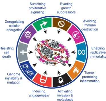
The genomes of mammalian cells carry all information needed to create a molecular machinery that regulates proliferation, differentiation and apoptosis (Ponting,2008). However, genomes of cells are altered by various mechanisms which can lead to mutations of encoded genes. These mutations range from point-mutations to translocation of whole chromosomes. Due to these changes, cells can acquire new phenotypes which progressively drive the transformation of normal cells into malignant neoplasms (Preston-Martin et al.,1990). Furthermore, it is anticipated that tumorigenesis is a multi-step process that needs several alterations to take place (figure 1.1, Hanahan and Weinberg 2000,2011). Once cells have overcome the defense mechanisms that usually work against these characteristics, malignant growth arise.

Two main classes of tumors are known: benign– and malignant tumors. Benign tumors grow only locally confined and do not invade adjacent tissues, whereas malignant tumors grow more aggressive and do invade the nearby tissue. Furthermore, malignant tumors might release cancer cells into the blood stream which can reach the lymph nodes as well as distant sites of the body to finally form secondary tumors known as metastases. These

 Introduction

Figure 1.1: Capabilities acquired during tumorigenesis. (Reprinted fromHanahan and Weinberg (2011), Copyright (2011), with permission from Elsevier)

metastases spawned by the primary tumor are responsible for approximately 90% of cancer-related deaths (Pisani et al., 1999).

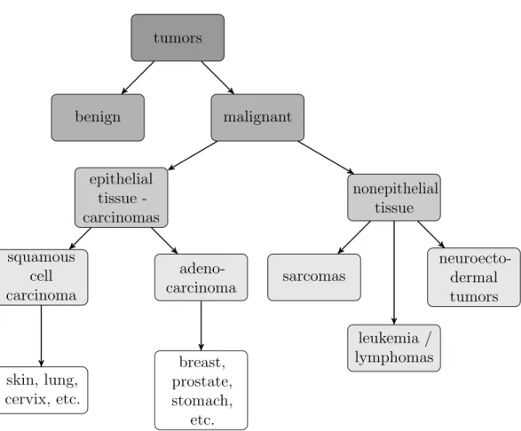
Tumors are further classified dependent on the tissue they arise from (figure1.2, Weinberg 2006). The majority of human cancers are carcinomas that emerge from epithelial tissue (Pisani et al., 1999; Jemal et al., 2010). Carcinomas are further classified into two subgroups: squamous cell carcinoma and adenocarcinoma. Squamous cell carcinoma arise from epithelial cells that form protective cell layers, i.e. they seal the cavity or channel that they line in order to protect underlying cells. The second class are adenocarcinoma which originate in epithelial cells that are specialized in secreting substances into the ducts or cavities they line.

. Clinical Cancer Research  tumors benign malignant epithelial tissue -carcinomas squamous cell carcinoma skin, lung, cervix, etc. adeno-carcinoma breast, prostate, stomach, etc. nonepithelial tissue sarcomas neuroecto-dermal tumors leukemia / lymphomas

Figure 1.2: Classification of most common tumor types (according to Weinberg 2006). Most malignant tumors arise from epithelial tis-sues (approx. 80%). These so-called carcinomas are split into two groups: squamous cell carcinoma and adenocarcinoma. All other, non epithelial tumors, are assigned into three major groups: sarcomas, leukemia/lymphomas and neuroectordermal tumors like gliomas, etc.

1.1.1

Breast cancer

Breast cancer belongs to the class of adenocarcinoma and is by far the most common form of cancer in women (Jemal et al., 2010). Breast cancer often forms metastases and this has made it the second leading cause of cancer-related death in women (Weigelt et al.,2005).

Breast cancer is mostly diagnosed by mammography or breast examination. Once diagnosed, patients usually undergo surgery to remove the primary tumor. After surgery, clinico-pathological parameters are used to estimate

 Introduction the progression status and the risk of recurrence. These estimates are used to decide whether a patient needs to undergo adjuvant treatment, which usually consists of systemic chemotherapy, radiotherapy or targeted treatment. The adjuvant treatment aims at eliminating all microscopic cancer cells and decreasing the risk of recurrence. However, due to the heterogeneity of breast cancer current clinico-pathological markers like lymph node status, tumor size or differentiation status are not appropriate for predicting the aggressiveness of the disease (Tavassoli and Devilee, 2003; Carter et al., 1989; Elston and Ellis,1991). Indeed, women with the same clinico-pathological characteristics can have a notably different courses of disease. Hence, lots of patients are overtreated and suffer from the substantial side-effects of chemotherapy (Eifel et al., 2001). Therefore, new prognostic markers, that are able to estimate the probability of recurrence at the time of diagnosis are urgently needed.

It is widely accepted that molecular alterations lead to cancer-development (Garnis et al., 2004). Microarray technologies allow to measure the expression of thousands of genes in parallel. By associating these expression profiles with the clinical outcome of patients, new biomarkers can be discovered. Due to the heterogeneity of breast cancer this approach is more promising than just correlating a few clinico-pathological markers or combinations thereof to the course of disease (Weigelt et al.,2005). The aim is to use gene expression profiles for tailored adjuvant therapy.

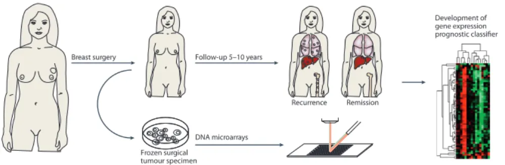
Retrospective studies are commonly applied to identify novel prognostic markers for improving risk stratification of breast cancer patients (figure

1.3). To this end, biomolecules are extracted from surgical tumor specimens of cancer patients. In particular, extracted RNA is mainly used to study large scale gene expression profiles using DNA-microarrays. In the retro-spective study design, RNA profiles can be correlated to long-term (5-10 years) clinical follow-up data of breast cancer patients. Relapse events (local recurrence, distant metastases) are commonly used as the primary clinical endpoint to identify novel molecular biomarkers using bioinformatic analyses. These analyses commonly consist of unsupervised (clustering) or supervised learning (classification) approaches. In the ideal case, markers identified by

. Clinical Cancer Research  Development of gene expression prognostic classifier Frozen surgical tumour specimen Follow-up 5–10 years Breast surgery DNA microarrays Remission Recurrence

Figure 1.3: Course of a retrospective study for the development of a prognostic marker. (Adapted by permission from Macmillan Publishers Ltd: Nature Reviews Cancer (Sotiriou and Piccart, 2007), copyright (2007))

retrospective studies should also be tested in an independent prospective study (Ransohoff, 2005).

In the early twenty-first century, microarray studies led to the discovery of breast cancer subgroups. By applying unsupervised bioinformatic analyses to gene expression data,Perou et al. (2000) found portraits of four molecular different breast cancer subtypes: ERBB2-positive, normal breast-like, luminal and basal-like. ERBB2 positive breast cancer patients carry a characteristic amplification of a region on chromosome 17 that includes the ERBB2 gene. Due to this amplification ERBB2 itself but also adjacent genes as well as the ERBB2 pathway are overexpressed. The normal breast-like subtype expresses genes of non-epithelial cell origin. Luminal breast cancer samples are charac-terized by a high expression of the estrogen receptor (ER) and coregulated genes as well as other specific markers of luminal epithelial cells. The luminal subtype was later divided into luminal A and B, where subtype B has a lower expression of the ER-coregulated genes and a higher rate of proliferation associated with an adverse prognosis (Sorlie et al., 2001). The basal-like subtype commonly shows high EGFR expression and a loss of expression of the ERBB2–, progesterone– and estrogen receptors, respectively. It is important to note, that independent gene expression studies have confirmed that these breast cancer types are clinically distinct subgroups (Sorlie et al.,

2003), since they show substantially different clinical outcome and response to treatment (Rouzier et al., 2005).

 Introduction

1.1.2

Existing markers for breast cancer prognosis

Several gene-signatures for breast cancer prognosis have been suggested in recent years. Van ’t Veer et al.(2002) from the Netherlands Cancer Institute (NKI) in Amsterdam reported a multigene signature consisting of 70 genes (Mammaprint) that reliably predicts the likelihood of distant metastases in lymph node-negative tumors. Subsequent use of a cohort of 295 patients could validate the signature as being the best predictor for metastasis-free survival. Additionally, it has been shown that the signature is independent of factors like histological grade, age, tumor size and adjuvant treatment (van de Vijver et al.,2002).

Two years later, Wang et al. (2005) published a 76-gene signature ob-tained by a related approach as the one used by the group from Amsterdam. Although, both gene-signatures only had three genes in common, they showed similar performance and could be validated in an independent study with 302 patients conducted in the framework of the translational research network of the Breast International Group (Buyse et al., 2006; Desmedt et al., 2007).

It needs to be stressed, that one of the main reasons for the small degree of concordance in gene-signatures are correlation structures, inherently present in microarray measurements. Briefly, if a gene is highly correlated to the clinical outcome and thus is a good marker, all other genes correlated to that gene are in turn also good predictors of clinical outcome. However, depending on the patients present in individual training sets, this correlation might vary and hence the rank of correlated genes is highly unstable. This leads to unstable gene signatures that have only a few genes in common (Ein-Dor et al., 2005). In addition, the utilization of different microarray platforms for measuring the gene expression might also lead to a decreased reproducibility. Further sources of variation might be differences in bioinformatic algorithms used for normalization and marker discovery. Another reason for the small overlap is the limited statistical power, i.e. too small sample sizes for training and testing of algorithms in order to identify disease-associated genes (Ein-Dor et al.,2006).

. Biomarker discovery using bioinformatics  Although, individual signatures for breast cancer prognosis contain differ-ent genes, their ability to predict the outcome on independdiffer-ent patidiffer-ent cohorts is similar (Tan et al., 2003; Fan et al., 2006). Nevertheless, individual genes, present in these signatures, are not necessarily connected to the underlying disease. This hampers our understanding of underlying mechanisms. Hence, there is a pressing need to develop new algorithms capable of identifying gene-signatures correlated to the intrinsic biology that are still able to predict the course of cancer with high accuracy.

1.2

Biomarker discovery using

bioinformatics

Microarray analyses have become a standard means for assessing genome-wide gene expression measurements of biological systems. Bioinformatics uses statistical, mathematical and computational methods for analyzing and processing the resulting data. Bioinformatic analyses are a crucial step for achieving biological understanding. Gene expression measurements of differ-ent classes of samples raise the vital question of how to discriminate these classes and how to determine meaningful biomakers, i.e. signatures of genes. Therefore, the development of novel bioinformatic algorithms is essential for increasing the accuracy of biomarkers and guide the biological understand-ing. In clinical cancer research, for example, it is known that most cancer treatments are only suited for a specific subgroup of patients. Therefore, bioin-formatic algorithms can facilitate the development new predictive biomarkers that help to identify patients that would benefit from a certain treatment. Other classes of biomakers are diagnostic biomarkers, that help identifying the absence or presence of a disease, and prognostic makers determine the likelihood of a relapse (Biomarkers Definitions Working Group, 2001).

Given these diverse types of biomarkers and applications, an impressive collection of bioinformatic tools has been developed for identification and validation of new markers. These methods are either supervised, i.e. the

 Introduction classes are known, or unsupervised when the class of individual samples is unknown. A well known class of unsupervised methods arecluster algorithms that can, for instance, be used for the identification of tumor subtypes. The class of supervised learning algorithms include classification methods that use patterns of carefully phenotyped samples to learn the characteristics of individual groups. Examples of these tools include algorithms like the support vector machine (SVM, Boser et al.,1992),k-nearest neighbors (kNN, Duda and Hart,1973), the nearest shrunken centroid classifier (PAM, Tibshirani et al., 2002), decision trees (Quinlan, 1986) and many others (Dudoit et al.,

2002).

However, an intrinsic problem that usually occurs when conducting mi-croarray analyses is that the number of genes, present on the chip, is much larger compared to the number of patients included in the study. This problem is well known in the field of machine learning and sometimes referred to as the curse of dimensionality (Bellman, 1961). The large number of genes present on the microarray makes these analysis prone to the curse of dimensionality, since the classifier will most probably find a decision rule which works well on the training data. However, since most of the genes used by the decision rule are probably not, or only by chance, associated with the disease state, the performance of the decision rule is overestimate and it will perform worse on new samples.

One possibility to tackle this problem is merging the many available covariates into some few by using so-calleddimensionality reduction algorithms. The most famous of these methods is probably the principal component analysis (Pearson,1901). However, when molecular markers are sought this is not the preferable approach.

Another possibility to overcome the curse of dimensionality is to build the classifier exclusively on those genes that are of importance to the disease. However, these genes are not known a priori and, thus have to be selected by the learning algorithm. The task of selecting only a subset of genes is known asfeature selection (seeGuyon and Elisseeff,2003, for an overview). However, genes composing the final signature are usually selected independently of

. Biomarker discovery using bioinformatics  each other, although proteins are known to interact within protein complexes, signaling pathways, and higher-order cellular processes. The reason for this independent selection is that standard classification methods merely rely on gene expression data and score each gene individually for how well it discriminates different classes of a disease. Therefore, the final classifier may contain unnecessarily many genes with redundant information which may lead to decreased classification performance on new samples (Lee et al.,

2008). This is also one possible explanation, why gene signatures have only a few genes in common, even if they are designed to predict the same clinical outcome (Ein-Dor et al., 2005). Despite the instability, these signatures are usually not easy to interpret since the membership in the gene-signature is not necessarily a indicator of the importance of that gene in, for example, cancer pathology (Weigelt et al., 2005).

1.2.1

Pathway-based classification methods

Recent studies have demonstrated that standard classification methods can be improved in terms of accuracy as well as stability of selected genes by including a priori knowledge of interactions into the classification process. Here, the term ’interactions’ is rather loosely defined, i.e. it refers to any kind of interacting biological entities that might form a network, pathway or signalling-cascade. These pathways are used to build a graph structure with biological entities (i.e. genes or proteins) as vertices and edges representing any kind of interaction. The field of pathway-based classification is rapidly growing and several methods have already been described.

Chuang et al. (2007) integrate pathway knowledge from protein-protein interaction networks. Their algorithm randomly chooses sub-networks and assigns an activity score based on the expression level of the genes from the sub-net. Afterwards, sub-networks which are able to discriminate between the clinical endpoints are identified and subsequently used to build a classifier based on these networks.

 Introduction

Rapaport et al. (2007) define a new metric for gene expression measure-ments by using the matrix exponential function, which is similar to the diffusion kernel (Kondor and Lafferty, 2002). Their assumption is that most biologically relevant information is captured in the low-frequency component of expression profiles. Hence, the projection of the low-frequency component of an expression vector on the gene metabolic network should reveal areas of positive and negative expression on the graph that are likely to correspond to the activation or inhibition of specific branches of the graph.

The approach introduced byZhu et al.(2009) is called network-based SVM and uses a network-based penalty which leads to a grouped variable selection. This variable selection is achieved by penalizing the SVM objective function with an F∞-norm (Zou and Yuan,2008), instead of the commonly usedL1 or

L2 penalization. This norm forces the simultaneous selection or elimination of

a group of features from the same pathway. Zhu et al.(2009) treat neighboring genes in a graph as a group and construct their network-based penalty as the sum of F∞-norms of groups of neighboring genes-pairs.

Yousef et al. (2009) introduced an algorithm which uses the Gene Ex-pression Analysis Tool (GXNA, Nacu et al. 2007) to build clusters of genes which are connected. They use these clusters as input to a linear SVM, assign a weight to the clusters based on the importance to the classification and then remove the least informative clusters. The process of training the SVM and removing unimportant clusters is repeated until the maximum classifi-cation performance is reached. This algorithm is called Recursive Network Elimination (RNE), as it removes clusters of genes instead of removing single genes.

A method called PathBoost which is based on likelihood-based boosting was recently proposed by Binder and Schumacher(2009). Still others have been published by Bellazzi and Zupan (2007); Lee et al. (2008); Su et al.

. Biomarker discovery using bioinformatics 

1.2.2

Pathway databases for building graphs

The knowledge on interacting biological entities is usually stored in databases. Depending on the system described, different levels of background knowledge exist. The Gene Ontology (GO,Ashburner et al.,2000) consortium represents an initiative which provides a vocabulary on gene functions to facilitate the systematic usage of this knowledge. The graph associated with GO is a directed acyclic graph where the nodes are the vocabulary and the edges represent relations like ’is a’ and ’part of’. The GO is structured hierarchically, it has three top level annotations, being:

molecular function describing the function of a gene, e.g. kinase, phos-phatase or transcription factor;

biological process describing the process or pathway a molecule is involved in, e.g. cell death, cell cycle or MAP kinase pathway;

cellular component describing the part of a cell or cell structure in which a molecule is active, e.g. nucleus, ribosome or cell membrane.

Several databases have been created for storing and collecting gene-specific information in GO format. This data can be used to create a matrix of pairwise similarities or dissimilarities of genes. Subsequently, the matrix can be used to score the gene-gene interactions and incorporated into the biomarker discovery process. Several methods have been developed for this purpose (Fr¨ohlich et al.,

2007). An overview of methods for accessing and mining these annotations is given in Beißbarth (2004).

Although the GO initiative has been founded ten years ago, most informa-tion on gene funcinforma-tion is still hard to mine, since it is not stored systematically. However, first attempts have been made to add GO-based meta-tags to publi-cations (Vanteru et al.,2008; Doms and Schroeder, 2005). Another way is to manually curate the published information, as done by TransPath (Choi et al.,

 Introduction still others rely on text-mining tools for automated information extraction (Jensen et al., 2006; Agarwal and Searls, 2008).

Databases like KEGG (Kanehisa and Goto, 2000) or consensusPathDB (Kamburov et al., 2009), focus on the biological interactions defining the processes of living cells and summarize these in manually curated pathway models. There also exist more focused databases representing molecular interactions obtained by genomic techniques like transcription factor binding based on chip-chip data, e.g. TRANSFAC (Wingender, 2008) or JASPAR (Portales-Casamar et al., 2010), or protein-protein interactions based on

co-immunoprecipitation or yeast two-hybrid screening, e.g. HPRD (Prasad et al.,

2009), MINT (Ceol et al., 2010) or IntAct (Aranda et al.,2010).

1.3

Aim and organization of the thesis

The focus of this thesis was the development of methodology that enables classification algorithms to use graphs in combination with patient specific data for building decision rules and detecting biomarkers for risk prediction. We used the SVM, which is a supervised learning method that has shown its predominance over other methods and can easily handle high dimensional data (Furey et al., 2000; Brown et al., 2000). In combination with the recursive feature elimination algorithm (RFE,Guyon et al.,2002), the SVM is able to narrow down the number of genes needed to build the decision rule. However, this feature selection is merely based on mathematical criteria. Here, we tried to incorporate prior biological knowledge in the form of a graph structure to improve the classification performance and the interpretability of selected genes. The graphs needed for this algorithm can be build from any of the databases mentioned in the previous subsection (see Porzelius and Johannes et al., (2011)). The assumption was, that the novel algorithm benefits from the pathway knowledge since genes are no longer treated as independent.

To make the work more self-contained, the prerequisites and theoretical foundations needed to understand the results are outlined in chapter 2. In

. Aim and organization of the thesis  section2.1the basics of SVMs are briefly introduced, before section 2.2shows how feature selection is performed when using SVMs. Sections2.3and2.4deal with model assessment and introduce the Receiver Operator Characteristic for evaluating classifiers. Afterwards (in section 2.5), we show how genes can be ranked by using a modified version of Google’s PageRank algorithm deployed on gene networks. The remainder of the chapter shows how the gene networks were created and introduces the breast cancer gene expression data sets, that were used for evaluating the algorithm.

Chapter 3 shows the results, starting with our newly developed algorithm called Reweighted Recursive Feature Elimination (RRFE, Johannes et al.,

2010). Section 3.1.1 outlines the results obtained by using RRFE, i.e. that RRFE selects interpretable genes (section 3.1.1.1), increases the classification performance as well as the overlap between marker-genes in gene-signatures obtained from different experiments (section3.1.1.2) and that it is predominant over other classifiers (3.1.1.5). The second part of the Results chapter deals with a software package that was developed to facilitate the usage of pathway-based classification methods (Johannes et al., 2011). We implemented the novel RRFE methods as well as two other methods that are able to useprior knowledge.

Chapter 2

Material and Methods

2.1

Support Vector Machines

2.1.1

Introduction

The goal of this section is to introduce support vector machines, the classifica-tion algorithm that has been used in this work. The support vector machine (SVM, Boser et al. 1992) is a statistical learning method for building

classi-fication models. It belongs to the separating hyperplane classifiers. These algorithms try to find a linear decision boundary which separates the data as well as possible.

The section is organized as follows: 2.1.2introduces separating hyperplanes and section 2.1.3will outline the maximum margin principle which is key for support vector machines. Afterwards, section 2.1.4 will show how to solve the support vector classification problem.

 Material and Methods x2

x1

w

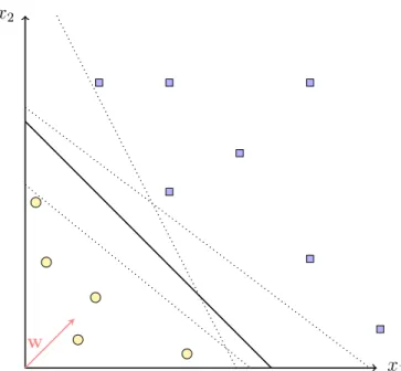
Figure 2.1: Example of a linear separating hyperplane in R2. The

dotted lines indicate, that even when the data is perfectly separated by the black line, there are infinitely many other solutions.

2.1.2

Linear hyperplanes

AssumeHbeing a Hilbert space andxi, . . . ,xn∈ His a set of pattern vectors with labels yi, . . . , yn∈ {±1}. In H any hyperplane can be defined as

{x∈ H :f(x) =wTx+b= 0}, w∈ H, b ∈_R. (2.1) Here, w is the vector normal to the hyperplane and b is the offset from the origin. An example of such a hyperplane in _R2 is given in figure 2.1. Since (2.1) separates H in two half-spaces of points classified as positive H+ _{= {x: f(x) ≥ 0} and negative H}− _{={x :f(x)< 0} it corresponds to} adecision function. Thus, a new sample with input vector xis assigned to class sgn(f(x)) = sgn(wT_{x+b). For a candidate functionf one can check} for each example (xi, yi) if it was correctly classified, i.e. 0 ≤yif(xi) or not. One possibility to choose f is called empirical risk minimization, that is, one tries to minimize the amount of wrongly made decisions on the whole set of examples (xi, yi), i = 1, . . . , n. However, there are infinitely many

. Support Vector Machines  of such linear hyperplanes that perfectly separate the toy data as shown in figure 2.1. Therefore, one could additionally demand that the examples should be classified with strong confidence, which leads to the principle of maximum-margin hyperplanes.

2.1.3

Maximum margin principle

If one considers (2.1) it is obvious that there is still the freedom to multiply w and b with the same non-zero constant in order to recover an equivalent hyperplane. In order to remove this scaling freedom, the SVM searches for the canonical hyperplane. It maximizes the margin between both classes, i.e. the distance to the points closest to it. The canonical hyperplane is defined by the pair (w,_b ˆb)∈ H ×_Rwhich is scaled such that the point closest to the hyperplane has a distance of 1_/k

wk: min i=1,...,n wTx_i+b = 1 (2.2)

for all xi, . . . ,xn ∈ H. Thus, the width of the margin is exactly equal to

2_/k

wk. An example of a maximum-margin hyperplane is shown in figure 2.2.

The idea behind maximum-margin hyperplanes is that making the margin as big as possible minimizes the bound on the risk (cf. Boser et al. 1992;Vapnik and Cortes 1995).

2.1.4

Support vector classification

The last two sections have introduced some of the foundations of SVMs. In this section it will be shown how the support vector classifier can be computed. In the ideal case one wants to classify all examples correctly with high confidence using a linear function like (2.1) with the constrains of (2.2). In a mathematical formulation this corresponds to maximizing 2_/k

wk under the constraints 1 ≤ yif(xi) =yi(wTxi +b) for i = 1, . . . , n. However, it is intuitive that this perfect separation of the data by a linear function might

 Material and Methods x2

x1

w

Figure 2.2: Maximum margin hyperplane. The dashed lines show the borders of the margin. Its width is exactly 2/kwk. The red line indicates the weight-vector of the hyperplane which is orthogonal to it. The examples that lie on the margin are called support-vectors.

not always be possible. This is particularly true for biological data, which is known to be quite noisy (Tilstone, 2003; Febbo and Kantoff, 2006). Thus, this section focuses on the soft-margin SVM implementation. In contrast to the hard-margin version it allows for some fraction of misclassification.

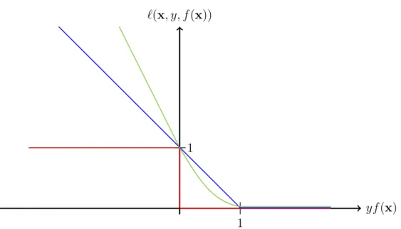
Even though a perfect classification might not be possible one wants to find the best possible solution. Therefore, a criterion to assess the quality of the estimate is needed. This is assessment is usually done by optimizing some functional. However, this type of function should fulfill certain criteria like having its minimum at zero, since a correct prediction should result in a zero penalty. Additionally, it should not only count misclassifications but also take into account the confidence of the estimate. A well known class of functions which is well suited for this type of problem is known as loss functions. They measure the loss generated by a function f for a given training example x with known class-label y.

. Support Vector Machines  Definition 2.1.1 (Loss Function). Assume the triplet (x, y,sgn(f(x))) ∈ H × {±1} × {±1} being a training example, a class label and a prediction, respectively. Then a map `:H × {±1} × {±1} →[0,∞) with the property that `(x, y, y) = 0 for all x∈ H and y ∈ {±1} is called a loss-function.

The most intuitive way to measure the loss is to simply count the fraction of misclassified examples. This is achieved by the binary or 0–1 loss:

`(x, y, f(x)) =    0 if y= sgn(f(x)) 1 otherwise. (2.3)

However, one might also want to involve the confidence with which the classification was carried out. That leads to the hinge loss (Bennett and Mangasarian, 1992): `(x, y, f(x)) = max(0,1−yf(x)) =    0 if yf(x)≥1 1−yf(x) otherwise. (2.4)

The hinge loss already takes into account the belief in the prediction. However,

Cristianini and Shawe-Taylor (2000) have shown that the squared version of (2.4) can be minimized more easily:

`(x, y, f(x)) = max(0,1−yf(x))2. (2.5) Examples of these loss functions are given in figure 2.3. The 0–1 loss function only punishes erroneous predictions. In contrast, the hinge and the squared hinge loss incur no penalty as long as the example is classified correctly with high belief but increase the penalty slowly when the belief decreases.

Having introduced the squared loss function, the final optimization problem can be defined: minimize w,b 1 2kwk 2 _+C n X i=1 `(xi, y, f(xi)) (2.6)

 Material and Methods

yf(x) 1

`(x, y, f(x))

1

Figure 2.3: Example of three different loss functions (cf. Sch¨olkopf et al. 2004). Blue: Hinge Loss; Red: 0–1 Loss; Green: squared Hinge Loss.

Equation (2.6) maximizes the margin (by minimizing kwk) and minimizes the hinge loss. Hence,C > 0 is a tuning parameter that controls the tradeoff between loss induced by ` and size of the margin. Thus, a large value of C leads to a smaller margin but increases the number of correctly classified examples with high belief. ForC → ∞ the hard-margin SVM, that allows no errors, is achieved.

However, there are several advantages to not directly minimize (2.6) since neither (2.4) nor (2.5) is differentiable (Chapelle, 2007). Therefore, one usually reformulates (2.4) and introduces n so-called slack variables

ξ = (ξ1, . . . , ξn) that measure the degree of misclassification. This leads to the primal optimization problem:

minimize w,b,ξ 1 2kwk 2_+C n X i=1 ξi (2.7)

. Support Vector Machines  subject to

ξi ≥`(xi, y, f(xi)), ∀i= 1, . . . , n.

To see that (2.6) and (2.7) are equivalent one needs to understand that the minimum of (2.7) with respect to ξi is reached when ξi takes its minimal value, which is `(xi, y, f(xi)). The next step is to split the squared hinge loss function (2.5) into two constraints, namely ξi ≥0 andξi ≥1−yi(wTxi+b). Thus (2.7) becomes: minimize w,b,ξ 1 2kwk 2_+C n X i=1 ξi (2.8) subject to ξi−1 +yi(wTxi+b)≥0 and ξi ≥0 ∀i= 1, . . . , n. (2.9)

Equation (2.8) is called anobjective function and (2.9) are calledinequality constraints. The combination of both (2.8) and (2.9) is known as aconstrained optimization problem and is subject to convex optimization theory. One convenient way to solve such constrained optimization problems is to introduce Lagrange multipliers. For each of the constraints (2.9) a positive Lagrange multiplier, sometimes also referred to as dual variable, has to be introduced. Hence, for each training example, α = (α1, . . . , αn) ≥ 0 represents the constraint ξi−1 +yi(wTxi+b)≥0, andβ = (β1, . . . , βn)≥0 denotesξi ≥0. Note, that the rule is that for constraints of the form ci ≥0, the constraint equations are multiplied with positive Lagrange multipliers and subtracted from the objective function. Therefore, the Lagrangian has to be formulated

 Material and Methods as: LP(w, b,ξ,α,β) = 1 2kwk 2_+C n X i=1 ξi − n X i=1 αi[ξi−1 +yi(wTxi +b)] − n X i=1 βiξi (2.10)

LP has to be minimized w.r.t the primal variables (w, b,ξ) and maximized with respect to the dual variables (α,β) ≥ 0. Therefore, for fixed (α,β), LP is minimized as a function of (w, b,ξ) by setting the respective partial derivatives to zero: ∂LP ∂w =w− n X i=1 αiyixi = 0 (2.11) ∂LP ∂b = n X i=1 αiyi = 0 (2.12) ∂LP

∂ξ =C−αi−βi = 0 ∀i (2.13)

together with positivity constraintsξi ≥0,αi ≥0 and βi ≥0. Substituting (2.11) – (2.13) into (2.10) recovers Wolfe’s dual (Wolfe, 1961):

LD = n X i=1 αi− 1 2 n X i=1 n X j=1 αiαjyiyjxTi xj (2.14)

which has to be maximized subject to (α,β)≥0 under the constraints (2.12) and (2.13). Compared to (2.10) equation (2.14) is a simpler convex quadric optimization problem an can be solved with standard algorithms likeGill et al.

(1981). However, β does not occur inLD. Thus, it can be maximized as a function ofα. However, it must be ensured that for someβ≥0 the constraint (2.13) is met. This is the case if and only ifαi ≤C for all i= 1, . . . , n, since only then a βi ≥ 0 can be found such that C =αi+βi. This leads to the

. Support Vector Machines  following constraints on the dual optimization problem (2.14):

0≤αi ≤C and n

X

i=1

αiyi = 0, ∀i= 1, . . . , n. (2.15)

Since this is a convex optimization problem the Karush-Kuhn-Tucker (KKT,

Kuhn and Tucker 1951) conditions apply. In addition to (2.11) – (2.13) the KKT are:

yi(wTxi+b)−1 +ξi ≥ 0 (2.16) αi[ξi−1 +yi(wTxi+b)] = 0 (2.17)

βiξi = 0 (2.18)

∀i= 1, . . . , n.

In combination equations (2.11) – (2.18) uniquely define the solution to the SVM optimization problem.

After having found the α_b that maximizes (2.14) , βb can be calculated as:

b

βi =C−αbi ∀i= 1, . . . , n. (2.19)

After rearranging equation (2.11) the solution for the weight vector w_b of the hyperplane is given by:

b w= n X i=1 b αiyixi (2.20)

It is, however, worth mentioning that w_b is a linear combination of solely the support vectors, that is, only those points with Lagrange multiplier α_bi 6= 0. Hence, the hyperplane found by the SVM does not change when non-support vectors are removed from the training set. Moreover, it is important that all support vectors with a slack variable ξi = 0 lie on the margin (in-bound support vectors) and due to (2.13) and (2.18) are defined by 0<α_bi < C. All others (ξi >0, bound support vectors) have αbi =C. Equation (2.17) shows

 Material and Methods To predict the class membership of a new samplex∈ Hthe linear function

b f(x) = w_bTx+ ˆb= n X i=1 yiαbix T i x+ ˆb (2.21)

has to be formed. Subsequently, sgnfb(x)

can be used to predict the class of xas +1 or −1.

2.1.5

Kernels

Another advantage of Wolfe’s dual (2.14) that has not been mentioned in the previous section, is that the pattern vectors occur as dot products. This makes possible the use of so-called kernels that represent a similarity measure of the input patterns in a much higher (possibly infinite) dimensional feature space. The map from the input– into the feature space is usually defined as:

φ: X → H

x7→x:=φ(x).

(2.22)

Given this map, the kernel itself is defined as:

k(x, x0) :=hx,x0i=hφ(x),φ(x0)i (2.23)

The important point is, that the kernel (2.23) allows calculation of the dot product in the feature spaceH without having to explicitly compute the map

φ. This is also known as the kernel trick.

Even if the data already exists in a dot product space, as assumed in previous sections, it is still possible to apply a nonlinear map φ. This might change the representation of the data into one that better fits the problem. Additionally, a change of the mapφ leads to a new similarity measure, which allows one to create a large variety of learning algorithms. However, biological data, coming from microarray experiments, is already very high dimensional. Hence, this data is most often linear separable and there is usually no need

. Feature selection using support vector machines  to map the features into a space with even more dimensions.

The interested reader is referred toVapnik(1995);Burges(1998);Sch¨olkopf and Smola (2001);Sch¨olkopf et al. (2004) for more detailed introductions.

2.2

Feature selection using support vector

machines

2.2.1

Introduction

In machine learning applications, data usually consists of measurements of some quantity. Frequently, the measurements are referred to as features or variables. Each data point is represented as a vector of dimensionality n, where n is the number of features. For each feature vector there exists a class label, defining to which class the vector belongs to. For simplicity, only two-class problems will be considered here. The challenge now is to select a classifier which assigns correct class labels to the training patterns. Furthermore, it should also be able to predict the class membership of future examples with low error rate.

It is, however, unclear if the learning algorithm needs all features to unravel the dependency between data points and class labels. A large amount of uninformative measurements might indeed mask the relationship between informative features and class labels. Additionally, the performance of a learning algorithm is strongly dependent on the quality of the data and thus, noisy, redundant or unreliable measurements impair the learning process.

There are, at least, two types of preprocessing methods that can be used to improve machine learning techniques: feature construction and feature selection methods. Feature construction methods use existing measurements and combine those to reduce the dimensionality of the problem. A well known linear example of such a method is the principal component analysis (PCA, Pearson 1901). There also exist non-linear methods which are based

 Material and Methods on kernels (Sch¨olkopf et al.,1998).

Feature selection methods, on the other hand, try to select the best subset of features to solve the classification task. Feature selection is performed in order to eliminate uninformative variables which should, in turn, lead to a better generalization performance, that is a better classification performance on previously unseen patterns. In addition to this, a reduced set of features may also give a better insight into the underlying model to be learned and a computational speedup. Other benefits might be cost reduction, in biological applications for example where only a smaller subset of genes has to be measured to detect a particular disease with the same accuracy as before (Rakotomamonjy, 2003). The goal of cost reduction cannot be reached with feature construction methods. The remainder of the section will focus on the task of feature selection.

2.2.2

Heuristics for feature selection

The task of identifying the optimal feature subset can be viewed as a search problem. Each state of this search consists of one possible feature subset. Due to the large number of features, this search space is usually high dimensional. Thus, it is obvious that this task can only be accomplished by usingheuristics, since there are 2n possible subsets for n features. Nevertheless, the nature of this heuristic needs to be defined by the following four characteristics:

First, the direction of the search has to be determined. One can either start with an empty model and iteratively take new features into the model, this process is known as forward selection. The reverse of this process, calledbackward elimination, starts with the complete model and discards one variable after the other (Neter et al., 1990).

Since it is known that an exhaustive search through the whole space is impractical the second issue is to organize the search. One possibility to do this is by using greedy methods that traverse the space. One possible approach is known as stepwise selection or elimination, and consider both

. Feature selection using support vector machines  adding and discarding variables at each step of the search. By doing so, it is possible to undo previous decisions without explicitly keeping track of the search path. In the end, all states generated can be considered and the one with best performance can be selected. Alternative methods, that are not greedy but still tractable, are best-first search or beam search, for example.

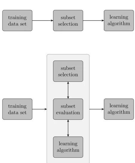
The third point is related to the approach used to evaluate the performance of the subsets. Again, two distinct strategies can be distinguished (figure2.4,

John et al. 1994). Filter methods treat the features independent of the selected learning algorithm. Thus, these methods merely rely on characteristics of the training set to include certain features and discard others. One example of such methods are statistical techniques, that compute a dependency between features and class labels, like Pearson’s correlation coefficient, wilcoxon– or t–statistics (Golub, 1999; Furey et al., 2000; Tusher et al., 2001; Hastie et al., 2009). Wrapper methods, on the contrary, select a certain amount of features and use this subset to run the learning algorithm on the training data. Afterwards the performance of each feature-subset is evaluated, which makes necessary the choice of a proper goodness-of-fit measure.

The last aspect to consider is a proper criterion to end the search through the space of feature subsets. When using filter methods this criterion might be to order features according to some relevance score and try different breakpoints. For wrapper methods the search could be continued until the accuracy starts to decrease or the search reaches the other end of the search space and select the best subset. For more details confer Langley (1994).

To this end, no assumption has been made about the underlying learning method. However, lots of progress has been made in the field of SVMs which are not equipped with an embedded feature selection (cf. section 2.1). However, several groups have developed feature selection algorithms for SVMs. For biological data, Moler et al.(2000) for instance, introduced a naive Bayes relevance (NBR) score to select informative features. Given the value of a gene and using Gaussian assumptions, the NBR score calculates a features’ probability of belonging to class one or two. The larger the probability, the more distinct is the expression of that feature and the more likely it is to be

 Material and Methods training data set subset selection learning algorithm training data set subset evaluation subset selection learning algorithm learning algorithm

Figure 2.4: Comparison of filter- and wrapper methods for subset selection (cf. John et al. 1994). The upper panel shows a filter method; it selects the subset of features independent of the learning algorithm. The lower panel shows a wrapper method. Here, the selected subset is evaluated using the learning algorithm. It is worth noting, that this inner evaluation has to be performed on an independent test set using cross-validation, for example.

. Feature selection using support vector machines  a good marker. In another work, Segal et al. (2003) used p-values obtained from studentst-test to rank genes and subsequently choose a certain number of most important genes to train the model. Both methods follow the goal of selecting certain features, but none of them considers important interactions but rather treats features as independent.

2.2.3

Recursive Feature Elimination

To overcome the above-mentioned problems, Guyon et al. (2002) introduced a wrapper method called Recursive Feature Elimination (RFE). For SVMs with a linear kernel, RFE uses kwk2_{, the squared norm of the weight vector}

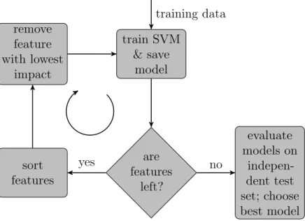
of the SVM hyperplane, as a ranking criterion for the importance of a feature. The authors proposed the following 4 steps (figure 2.5):

1. Train SVM on training data.

2. Rank features according to kwk2_.

3. Discard the feature with smallest impact from the training data.

4. If more than one feature is left go to 1, otherwise stop.

To formally calculate the influence of the kth feature on the squared weight vector norm, equation (2.14) can be used:

kwk2− kw(k)k2 = n X i=1 b αi− 1 2 n X i=1 n X j=1 b αiαbjyiyjhxi,xji − n X i=1 b α(_ik)+1 2 n X i=1 n X j=1 b α(_ik)α_b(_jk)yiyjhx(_ik),x(_jk)i (2.24) = 1 2 n X i=1 n X j=1 b αiαbjyiyjhxi,xji − n X i=1 n X j=1 b α(_ik)α_b(_jk)yiyjhx (k) i ,x (k) j i (2.25)

 Material and Methods train SVM & save model remove feature with lowest impact are features left? sort features evaluate models on indepen-dent test set; choose best model training data yes _no

Figure 2.5: Recursive Feature Elimination workflow. This chart explains the workflow of the RFE algorithm. First, the SVM is trained on the training data set, as long as features are left these are ordered and iteratively removed. In the end the performance of all models is evaluated on an independent test set in order to find the best one.

The notationc(k) denotes thatkth feature has been removed from vector c. Note, that the vector multiplication xT_i xj in (2.14) has been exchanged by the dot product hxi,xji. To simplify the calculation and reduce calculation time, Guyon et al. assume α_b(_ik) to be equal to α_bi.

After calculating (2.25), the features can be ordered according to their importance (high value means more important). Guyon et al. recommended removing chunks of genes to speed up the procedure. Hence, as a next step a specific amount of features from the bottom of the ordered list needs to be discarded. The process of training the SVM, calculating (2.25) and removing a specific amount of potentially uninformative features is repeated until the set of surviving features is empty. In practice, all trained classifiers obtained at step 1 are saved in order to afterwards examine their performance on an independent test set and thus identify the optimal number of features. This can, for example, be done by cross-validation or by using a theoretical concept like the span estimate (cf. section 2.3).

. Assessment and selection of models 

2.3

Assessment and selection of models

2.3.1

Introduction

The performance of a classifier or any other learning algorithm on an inde-pendent test data set is known as its generalization performance. A detailed examination of this quantity is a prerequisite in practical applications, since it guides the choice of the learning algorithm or model. Additionally, it allows the estimation of its classification capability on yet unknown data. In the following section some details will be given in order to introduce a process called cross-validation that estimates the expected test error in section 2.3.3. The reader interested in more details is referred to Hastie et al. (2009).

2.3.2

Training- and test error

Let T denote a training set. The training error is defined as the average loss over T: err = 1 n n X i=1 `(xi, yi,fˆ(xi)) ∀ xi ∈ T (2.26)

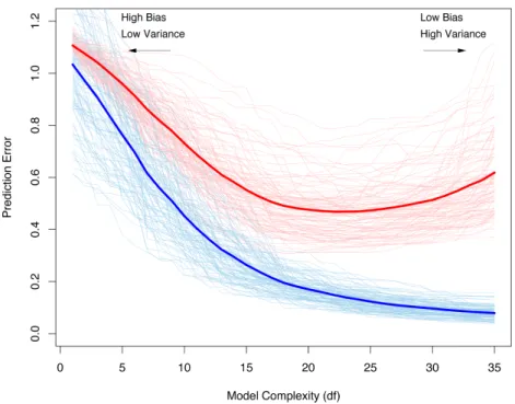
where ` is a loss function, for example the hinge loss (2.4). Usually one is more interested in the expected test error than inerr. However, the training error unfortunately is a bad estimate of the test error (figure 2.6), since the same data is used for fitting the model and assessing the loss it incurs. Thus, the estimate of err is biased downward. It is a too optimistic estimate of the expected generalization error. If the model complexity is increased enough the training error can become very small, or even zero. This will, however, lead to a highly overfitted model which will generalize only very poorly.

The test-or generalization error on an independent test sample is defined as:

 Material and Methods

Figure 2.6: Dependency of the expected training- and test error on the model complexity, shown as solid blue and red curves, respectively. The light blue and red curves show the training- and test error for 100 training sets of size 50 each. All models have been obtained by the lasso (figure courtesy ofHastie et al. 2009).

wherex0 andy0is a previously unknown test-point. Since ˆf has been obtained

by training on the fixed set T, the estimate ErrT is only valid given this particular training set. Figure 2.6 shows the generalization error for 100 training sets as light red curves. The expected- or average test error is given by:

Err = E[`(xi, yi,f(xˆ i))] =E[ErrT] . (2.28)

Equation (2.28) shows that this quantity is no longer dependent on a specific training set but rather averages over all possible training sets. It is shown as solid red line in figure 2.6. In the remainder of the section the goal is to efficiently approximate the expected test error (2.28).

. Assessment and selection of models 

2.3.3

Cross-Validation

Cross-validation (CV,Mosteller and Turkey 1968;Geisser 1975; Kohavi 1995) is one possible method that efficiently re-uses the given data in order to approximate the expected test error of a previously chosen model. However, it is worth noting that there are several goals CV can be used for:

Model selection: Here, several models of the same learning algorithm are compared in terms of their estimated performance in order to choose the best one.

Model assessment: Once, the best model has been chosen, the task of model assessment is to give an estimate on its generalization error.

In this work CV was used for accomplishing the second task. Model selection was performed using a theoretical concept, which uses an analytical expression to calculate an upper-bound on the test error (cf. section 2.3.4 for more details).

InK-fold cross-validation the data is randomly split intoK almost equally sized subsamples. For thekth subsample the model is fitted on the otherK−1 parts of the data. Afterwards, the model is used to predict the class labels of the examples in the kth subsample. Thus, the estimate of the prediction error through cross-validation is given by:

CV( ˆf) = 1 n n X i=1 `(xi, yi,fˆ−κ(i)(xi)). (2.29)

Where κ : {1, . . . , n} → {1, . . . , K} is an indexing function that defines to which subsample of the data sample i was assigned to. Thus, ˆf−κ(i) denotes the fit computed on the training data after having removed the subsample i belongs to. Common choices are K = 5 or K = 10 (McLachlan et al.,

2005). The condition K =n leads to theleave-one-out (loo) cross-validation estimate, CVloo, and κ(i) =i. CVloo is known to be the best approximation

 Material and Methods

Brailovsky,1969).

However, (2.29) is still only a point estimate of the expected generalization error (2.28). To reduce the variance of the estimate it is common to repeat theK-fold cross-validation several times with different split positions. Again, common choices are 5 or 10 repeats.

2.3.4

The Span Estimate

As introduced in the last section, cross-validation is used to estimate the generalization performance of a classifier trained on some training data. However, most learning algorithms have one or more tuning parameter which need to be optimized as well. An example of such a tuning parameter is the constantC in (2.6) or the optimal number of features. The problem of finding a function with parameters that minimize the expected error on the test data is called model selection. However, the number of parameters determine the size of the space of possible functions. Intuitively, the model selection demands several, nested, validations. The degree of nestedness of cross-validations, again, depends on the number of parameters to choose and can, thus, be a quite time-consuming method. In practice the naive strategy to exhaustively search the parameter space for the best solution becomes intractable. Thus, several authors have proposed methods to approximate an upper bound for the loo–error, CVloo( ˆf), of a classifier (Jaakkola and

Haussler,1999;Chapelle and Vapnik, 2000a; Opper and Winther, 2000). In this work, a quantity, called the span of the support vectors (Chapelle and Vapnik, 2000b) was used in order to calculate an upper bound on the number of errors made by the classifier. Let α_b = (α_b1, . . . ,αbn) be the solution

to the optimization problem (2.14). Chapelle and Vapnik have shown that for any support vectorxp the following equality is true:

yp( ˆf(xp)−fp(xp)) =αbpS 2

p. (2.30)

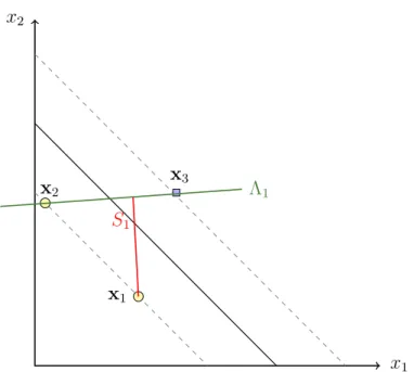
. Assessment and selection of models  x2 x1 x3 x2 x1 Λ1 S1

Figure 2.7: Example of the span of support vector x1 in R2. The

dashed lines indicate the margin. Λ1, shown by the green line, is the set

(2.31). The red line shows the span (2.32) of support vectorx1.

set and the set without the point xp, respectively. However, (2.30) is only true if in-bound and bound support vectors remain the same during the leave-one-out procedure. This limitation is obviously not always met. Nevertheless, the number of cases that violate this constraint is usually small compared to the number of support vectors. The proof of (2.30) can be found in Theorem 1 of Chapelle and Vapnik (2000a). In equation (2.30), S2

p is the distance of support vector xp to the set of constrained linear combinations:

Λp =    X {i6=p,0<bαi} λixi, X i6=p, λi = 1    . (2.31)

Formally, thespan of the support vector xp is defined as:

S_p2 =d2(xp,Λp) = min

x∈Λp

(xp−x)2, (2.32) which is the minimum distance from xp to Λp. A toy example is given in figure 2.7. By using the span estimate the numbers of errors made by the loo

 Material and Methods cross-validation can be calculated as:

T = 1 n n X p=1 Ψ(α_bpSp2−1) (2.33)

where Ψ is the Heaviside step function:

Ψ(x) =    1 if x >0 0 otherwise . (2.34)

2.4

Receiver Operator Characteristic

Receiver Operator Characteristic (ROC) graphs have a long tradition in machine learning applications (Spackman, 1989). They are mostly used for comparison of algorithms. Initially, however, they were used in signal detection theory (Egan,1975). Before introducing more details on the ROC space, some commonly used metrics for evaluation of classifier performance will be reviewed.

As said before, a classifier is a function which tries to map a vector x to a set of class labels,{±1} for example. There are models that do this in a discrete fashion, that is, produce output like −1 or +1. But there also exist classifiers that generate a continuous output, that is one needs to apply a cutoff in order to assign an instance to one or the other group. Assuming two classes, a classifier can create the following assignments:

true positive (TP): classify a positive instance as positive.

false negative (FN): classify a positive instance as negative.

true negative (TN): classify a negative instance as negative.

. Receiver Operator Characteristic  True Positive False Positive False Negative True Negative p p’ n’ P N’ N P’ n actual value prediction outcome total total

Figure 2.8: A 2 by 2 confusion table (cf. Fawcett 2004).

These class assignments can be written into a contingency table (figure

2.8). Using this information a variety of quality measures can be computed, some of which are shown in table 2.1.

The ROC space is spanned by 1−specificity (F P R) on the x-axis versus the sensitivity (T P R) on the y-axis. An example of a ROC graph is given in figure 2.9. The discrete classifier, mentioned above, leads to a single contingency table and thus to exactly one point in the ROC space. Whereas the continuous method allows one to vary the cutoff for inducing the (binary) classification rule from +∞ to −∞and thereby to traverse the ROC space from the lower left to the upper right corner.

The procedure of a typical ROC analysis with such a varying cutoff will be outlined by using the data from table 2.2 (see also Fawcett 2004). Figure

2.10 shows the resulting ROC graph. Table 2.2 carries information on 18 instances split into two classes (third column). The second column shows the continuous score used by a classifier to predict the class membership of each instance. This score could, for example, be the result of a SVM with hinge loss function (2.4). In the ROC graph a cutoff of +∞ corresponds to the

 Material and Methods

Name of measure Equation

sensitivity or true positive rate (TPR)

TPR = (TP+FN)TP

specificity or true negative rate (TNR)

TNR = _(FP+TN)TN = 1−FPR false positive rate (FPR) FPR = _(FP+TN)FP

false negative rate (FNR) FNR = FN (FN+TP)

accuracy (ACC) ACC = _{(FP+TN)+(TP+FN)}TP+TN

Table 2.1: Quality measures for evaluation of classifier performance (cf.

Fawcett 2004)

False positive rate

T rue positiv e r ate 0.0 0.2 0.4 0.6 0.8 1.0 0.0 0.2 0.4 0.6 0.8 1.0

Figure 2.9: Example of a ROC graph. Thex-axis denotes the false positive rate, whereas they-axis shows the true positive rate. The dashed diagonalx=yindicates the strategy of random guessing.

. Receiver Operator Characteristic  # score assigned by classifier real class label 1 0.51 + 2 0.45 + 3 0.44 + 4 0.43 + 5 0.40 -6 0.35 + 7 0.34 + 8 0.34 + 9 0.31 -10 0.29 -11 0.28 + 12 0.25 -13 0.25 -14 0.22 -15 0.21 -16 0.21 -17 0.20 -18 0.17 +

Table 2.2: Example data for a ROC analysis. The table shows 18 instances, 9 in class + and 9 in class−. The score comes from a learning methods that uses a continuous score to predict the class membership of