ECONOMICS
Agricultural Economics 49 (2018) 301–312
Spatial dependency and technical efficiency: an application of a Bayesian
stochastic frontier model to irrigated and rainfed rice farmers in Bohol,
Philippines
Valerien O. Pede
a,∗, Francisco J. Areal
b, Alphonse Singbo
c, Justin McKinley
a,d, Kei Kajisa
e aInternational Rice Research Institute (IRRI), DAPO Box 7777, Metro Manila, 1301, PhilippinesbSchool of Agriculture, Policy and Development, University of Reading, Whiteknights, P.O. Box 237, Reading, RG6 6AR, UK cInternational Crops Research Institute for the Semi-Arid Tropics (ICRISAT), BP 320, Bamako, Mali
dMonash University, Clayton, Australia eAoyama Gakuin University, 4-4-25 Shibuya, Tokyo, Japan
Received 13 June 2016; received in revised form 21 September 2017; accepted 2 November 2017
Abstract
We investigated the role of spatial dependency in the technical efficiency estimates of rice farmers using panel data from the Central Visayan island of Bohol in the Philippines. Household-level data were collected from irrigated and rainfed agro-ecosystems. In each ecosystem, the geographical information on residential and farm-plot neighborhood structures was recorded to compare household-level spatial dependency among four types of neighborhoods. A Bayesian stochastic frontier approach that integrates spatial dependency was used to address the effects of neighborhood structures on farmers’ performance. Incorporating the spatial dimension into the neighborhood structures allowed for identification of the relationships between spatial dependency and technical efficiency through comparison with nonspatial models. The neighborhood structure at the residence and plot levels were defined with a spatial weight matrix where cut-off distances ranged from 100 to 1,000 m. We found that spatial dependency exists at the residential and plot levels and is stronger for irrigated farms than rainfed farms. We also found that technical inefficiency levels decrease as spatial effects are more taken into account. Because the spatial effects increase with a shorter network distance, the decreasing technical inefficiency implies that the unobserved inefficiencies can be explained better by considering small networks of relatively close farmers over large networks of distant farmers.
JEL classifications: C01, C11, C23, C51, D24
Keywords:Rice farming; Spatial dependency; Bayesian approach; Efficiency
1. Introduction
Numerous attempts have been made to measure technical efficiency (TE) and other efficiency estimates in farming (Al-varez, 2004; Balde et al., 2014; Coelli and Battese, 1996; Hos-sain and Rahman, 2012; Idiong, 2007; Karagiannis and Tzou-velekas, 2009; Michler and Shively, 2014; Quilty et al., 2014); to this end, one of the common econometric approaches is the stochastic frontier analysis (Aigner et al., 1977; Meeusen and van den Broeck, 1977). Previous studies have contributed to the understanding of how large TE is; how different TE lev-els are among individual farmers; and what are the factors ∗Corresponding author. Tel.:+63-2-580-5600 (ext. 2721); fax:+63(2)
891-1236.E-mail address: [email protected] (V. O. Pede).
that underlie the differences. These studies generated useful policy implications for efficient farming, especially in devel-oping countries where wide productivity variations have been observed. Despite the aforementioned research, spatial depen-dency among farmers has yet to be adequately analyzed. Farrell (1957) expressed concerns about spatial factors such as how climate and location influence efficiency. Although the con-cerns existed at the time, the econometric techniques required to complete such an analysis were not available during the time of Farrell’s research. The importance of making use of spatial information in agricultural economics, and in particular the little attention paid to spatial autocorrelation in land use data has still been highlighted in more recent times (Bockstael, 1996).
C
Recent developments in spatial econometrics have made it possible to observe the spatial effects in the stochastic frontier analysis (Anselin, 1988; Areal et al., 2012; Glass et al., 2013, 2014, 2015; Tsionas and Michaelides, 2015). Furthermore, Druska and Horrace (2004) extended the estima-tor presented by Kelejian and Prucha (1999) and applied it to a stochastic frontier model for the panel data of 171 Indonesian rice farmers. Another innovation in this area was the adoption of the Bayesian paradigm in the estimation procedure (Schmidt et al., 2008). With this approach, Koop and Steel (2001) and Kumbhakar and Tsionas (2005) investigated geographical vari-ations of outputs and farm productivity for 370 municipalities in Brazil. Similarly, Areal et al. (2012) also investigated the spatial dependence of 215 dairy farms in England at a 10-km grid-square level using the Bayesian paradigm. All these studies have used a meso-level data to measure the spatial distribution of farmers.
Although these meso-level studies are valuable in recogniz-ing the importance of spatial dependency in agriculture, impor-tant questions surrounding this topic remain unanswered. To illustrate, one unanswered question is how and through what kinds of networks the spatial dependency of TE shows up at the farm level.
The purpose of this article is to investigate the role of spa-tial dependency in TE, using a unique micro-level farm panel dataset from individual rice farmers in Bohol, Philippines. We aim to identify the types of networks in which spatial depen-dency arises in TE. The data were collected for four consecutive rice growing seasons from 2009 to 2011, coupled with detailed geographical information to capture different kinds of networks among sample farmers. This data set allowed us to compare spatial dependency among two separate neighborhood struc-tures (residential neighborhood and farm plot neighborhood) in two different agro-ecosystem (irrigated and rainfed ecosys-tems). Taking advantage of the panel data structure, analyses were performed following a one-step procedure as described in Areal et al. (2012), which integrates spatial dependency into the stochastic frontier analysis with a Bayesian estimation ap-proach. The rest of the article is organized as follows. The next section provides some background information about the ma-jor characteristics of the two rice farming systems in Bohol. Section 3 presents the empirical model used to estimate the TE and the endogenous spatial effect of rice farming TE. Section 4 describes the data set used in this study. Section 5 presents the estimation results and discussions. Section 6 concludes and derives policy implications for rice farming productivity in Philippines.
2. Rice farming in Bohol
Rice production in Bohol consists of two agro-ecosystems: ir-rigated and rainfed farming. The Bohol Irrigation System (BIS) started its operation in 2009, currently spans 14 villages in 3 municipalities, and is expected to service as many as 4,104
hectares in the future (JICA, 2012). The BIS works through a gravity irrigation system composed of a reservoir dam, a main canal, secondary canals and laterals, turnouts, and farm ditches. Most of the farmers in the project site converted their rainfed plots to irrigated plots as long as their plots were accessible to the irrigation facilities. Our sample famers were randomly taken from these irrigated famers. The rainfed sample farmers were randomly taken from adjacent villages that have similar cultural and climatic background (Fig. 1). Rainfed rice farm-ing is conducted in a traditonal manner with moderate use of modern inputs and little use of machineries. The same sce-nario applied to the irrigated area until the start of irrigation in 2009.
Farmers in the irrigated area must form a water users group. A group consisting of 20 individual farmers on average and its members rely on the same intake gate on a canal and thus share irrigation water with each other. Since the location and the water supply capacity of each intake gate is determined by the capacity of the canal and the topography of the area, the size and composition of the water users group is basically determined exogenously. In addition, our field observation tells us that no farmer exchanged their plots in order to move to a particular water user group. This means that there is no self-selection behavior in the formation of the water user group.
Member farmers are expected to pay an irrigation service fee equivalent to 150 kg of paddy per hectare per season to the National Irriagtion Administration (NIA).1 The members of the water users group are expected to manage local irri-gation facilities collectively. Since they share irriirri-gation wa-ter, the synchronization of farming practices is needed among them. Meanwhile, rice farming under rainfed conditions is con-ducted more independently. In this regard, the opportunities for networking are more frequent, and the demand for strict coordination is higher among irrigated farmers than rainfed farmers.
In the study site, rice is the dominant crop and is cultivated twice a year. The Bohol Island belongs to a climatic area charac-terized by even rainfall distribution throughout the year. During our survey period of four agricultural seasons in two years (2009–2011), our study site experienced two weather shocks: severe drought in the second season and flood in the fourth season. Furthermore, rainfed areas suffered directly from these variations. Meanwhile, the water supply condition among irri-gated farmers was mitiirri-gated by the irrigation system, to some extent. Hence, the irrigated farmers suffered fewer water short-ages in the second season than the rainfed farmers. Since the BIS has no drainage system, all the famers suffered flood in the fourth season.
A notable feature of the study site, which is important in network analyses, is that the places of residence are rela-tively scattered over a wide geographical area; although we 1With a market price of Php 14–20 per kg, the 150 kg of paddy is equivalent
to about Php 2,500–3,000. As of February 2018 1USD=51 Php (Philipino Peso).
Fig. 1. Location of study sites designated by ecosystem. [Color figure can be viewed at wileyonlinelibrary.com]
can still find the center of a village where residences and small businesses are concentrated. Hence, the data presented in this study have wide geographical variations in residential networks, which is different from another type of common residential pat-tern in which residents are highly concentrated in a particular place.
3. Modeling
Since the seminal works of Aigner et al. (1977) and Meeusen and Van Den Broeck (1977), the stochastic frontier approach (SFA) has become the most commonly used method of mod-eling the production and measure efficiency of farm-level data. The SFA estimates the parametric form of a production function and recognizes the presence of two random error terms in the data. One component of the error term reflects the inefficiency in production while the other component represents the ran-dom effects outside of the producer’s control. The production frontier itself is stochastic since it varies randomly across farms due to the presence of the random error component.
Follow-ing the model proposed by Areal et al. (2012), the stochastic frontier production function for a balanced panel data assuming efficiency is constant over time2is defined as3:
yit=xitβ+zitθ+pitψ+vit−ui, (1) whereyitdenotes the production of farmi(i = 1,2, . . . , N) at
season t (t = 1, . . . , T) with T = 4; xit represents a
(N×T)×k matrix of inputs of production; zit is a N×m
2This is not an uncommon assumption to make especially when the time
series is relatively short as in this case (two years).
3A specification including time and its interactions was estimated but no
significant time effects were found. A referee has noted that the model does not include heteroscedasticity terms. This is an area that has not been explored within this context. We have run the nonspatial model and extracted the errors and the inefficiency terms. However, there is not a prior reason to believe that allowing for heteroscedasticity would make it necessarily a better model. We have conducted a Levene’s test on the errors to test whether the variance changes through the periods. We found that the variance for year 2 is actually different (P-value of<0.05), but the standard deviations for the years are not very different in absolute values: Year 1: 0.246; year 2: 0.306; year 3: 0.230; year 4: 0.239.
matrix of nonstochastic environmental variables (farmer’s level of education, household size, household head, being a female, remittance), associated with theith farm at thetth observa-tion (farm-specific variables);pit is aN×(T −1) matrix of
dummy variables for periods 2–4;β,θ,andψare respectively k×1, (T −1)×1 andm× 1 vectors of unknown parameters to be estimated;vitis the random error, andui represents the inefficiency of theith farm. Stacking all variables into matrices we obtain:
y=xβ+zθ+pψ+v−(u⊗1T), (2) where the inefficiency term in the standard efficiency analy-sis usually assumeuto follow an exponential of half-normal distribution. However,u can be made spatially dependent by defining it as:
u=ρW u+u,˜ (3)
whereW is a weight matrix;ρis the spatial coefficient, which is assumed to be between 0 and 1; anduand ˜uare latent vari-ables whose distributional form is unknown. In the context of farming,ρW ucaptures the effects of shocks spreading among neighboring farmers through similarity in socioeconomic, agro-ecological, and institutional backgrounds of the group defined byW.
Estimation of spatial models requires specification for the spatial structure of observation units considered in the study. As such, a distance-based weight matrix,W, of a Boolean type with elementswijwas defined as follows4:
wij= exp − dij2 s2 , (4)
where dij is the distance in kilometers between the
resi-dence/farm locationi and the residence/farm locationj; s is the distance from the residence/farm where spatial dependence may be relevant, i.e., the cut-off point of spatial dependence. Finding the appropriate cut-off distance is an empirical issue (Roe et al., 2002) that is commonly dealt with by estimating the spatial model using different cut-off distances (Areal et al., 2012; Areal and Riesgo, 2014; Bell and Bocksteal, 2000; Kim et al., 2003; Roe et al., 2002).
Therefore, we use two types of Bayesian models, one stan-dard SFA (nonspatial) and spatial models (with cut-off distance ranging from 100 to 1,000 m), which allow for an investigation of the relationship between spatial dependency and efficiency under different farm environments. Results from the nonspa-tial model and the spanonspa-tial model with the highest spanonspa-tial de-pendency are compared as follows. Once the farm efficiency estimates from both models are obtained, the efficiency per-centage change between the spatial and nonspatial model is calculated per household and farm environment (residential or farm plot). This allows us to explore how much accounting 4The weight matrixWis of dimensionN×Nand has 0 as diagonal elements.
for spatial dependency can help in explaining efficiency. If the area used to determine the neighborhood is relatively large, we may find spatial dependence; however this may not help in explaining efficiency. The same would occur if certain spatial effects that were accounted for are not relevant in explain-ing inefficiency, i.e., the spatial models in this case would be underperforming compared with the nonspatial models. Hav-ing found spatial dependency, a farm with a positive percent-age change in their efficiency level would indicate that such farm’s efficiency level would have been underestimated under the nonspatial approach (i.e., positive aspects such as sharing information that make farms more efficient were not taken into account). We would expect this to be the case of farms that work closely and share knowledge under similar environment. On the other hand, we may expect farms that work more independently to show lower levels of spatial dependence; and no or small percentage changes in cases where the spatial model matches the performance of the nonspatial model or even negative percentage change in cases where the nonspatial model out-performs the spatial models.
A translog functional form was chosen for the stochastic fron-tier production analysis. To explain, the translog is a flexible functional form that can be viewed as a second-order Taylor ex-pansion in logarithms of any function of unknown form. Unlike the Cobb-Douglas function, it imposes no restriction a priori on the elasticities of substitution between inputs and outputs. As mentioned above, some nonstochastic environmental variables were incorporated directly into the nonstochastic component of the production frontier accounting for changes in the production level.5
Thus, the variable,Education,was included and consists of the years of formal schooling of the primary decision-maker of the household; the variableSize, which is the total number of people living in the household; Gender, a binary variable taking a value of one when the household head is female; and
Remittance consisting of the ratio of remittance as it relates
to total household income. The first three variables capture the human capital endowment of the sample farmer: education for quality, size for amount, and the gender for advantage or 5There are two general approaches to incorporate nonstochastic
environmen-tal variables into technical efficiency analysis (Coelli et al., 2005). The first, the one used here, is to incorporate them in the nonstochastic part of the fron-tier model, whereas the second approach incorporates them into the stochastic component of the production frontier (Kumbhakar and McGukin, 1991). We have decided to use the first approach to distinguish between observed infor-mation, which is included in the production side and nonobserved information (spatial aspects) into the stochastic part of the frontier. However, following the suggestion of a reviewer we also conducted the second approach in which
Education,Size,Gender, andRemittanceare removed from the nonstochastic part and are used in a second stage as explanatory variables for the estimated efficiency. The coefficient estimates of the nonstochastic part are similar. Re-garding the explanatory variables for efficiency,Educationwas found to be associated with higher levels of efficiency in all cases whereasRemittancewas found to be associated with lower levels of efficiency (i.e., farmers recipients of relatively larger amounts of remittances were found to be less efficient than those receiving lower amounts of remittances). These results can be found in the Appendix.
disadvantage of female head. Educated farmers are generally assumed to have better farming capacity and access to informa-tion; therefore, they are more productive (Battese and Coelli, 1995). The amount of remittance indicates that farmers have alternative income sources other than rice farming. Hence, we hypothesize that remittance, which captures an unimportance of rice farming, has a negative effect on production levels.
The data for all inputs and outputs are normalized by their respective geometric means prior to estimation. This makes the model’s parameter estimates directly interpretable as elas-ticities that are evaluated at the geometric mean of the data. To cope with the great number of zero observations for fer-tilizer inputs, the procedure proposed by Battese (1997) was followed. The original variable for fertilizer was replaced with xk
it=max(xitk, Ditk) , where Ditk is a dummy variable defined
byDk
it= 1 ifxitk= 0 andDitk= 0 ifxitk>0. Thus, the final
estimable form of the translog stochastic production function becomes: ln yit =α0 + k αkln xitk +1 2 k j αkjln xitk ln xitj
+βkDitk+θ1Educationit+θ2HHsizeit+θ3Genderit
+θ4Remittanceit+
4
l=2
ψlpl+Vit−Ui, (5) whereyis the output,tis a time index (t = 1, . . . , T),kandj are the inputs, andα0,αk,αkj,θ1,θ2,θ3, θ4, ψl, βkare the pa-rameters to be estimated. The symmetry property was imposed by restrictingαkj=αj k. TheUi are farm-specific inefficiency
terms as defined above. The estimation was conducted using a Bayesian approach that integrates the latent distributions ofu and ˜uinto the estimation process as defined in Eq. (3) (Areal et al., 2012). Thus, a standard form for the conditional likeli-hood function was assumed in efficiency analysis with a spatial component added to:
py|β, h, ρ, μ−u1,u˜ = N i=1 hT2 (2π)T2 exp −hε ε 2 . (6) By reparameterizing ˜y =[y+(I −ρW)−1u˜⊗1T] , x = x+z+p the expression for the conditional likelihood func-tion was obtained:
py|β,h,ρ,μ−u1,u˜ ∝hTN2exp −h 2( ˜y−xβ) ( ˜y−xβ). (7)
The prior distribution for the parametersβ, h, μ−z1, u, ρ˜ are an independent Normal-Gamma prior forβandh; the prior for μ−u1is assumed to be Gamma with parameters 2 and−ln(r∗), wherer∗is the median of the prior distribution, and the condi-tional distribution for ˜uis:
pu˜i|α, μ−u1 = u˜αi−1 μju (α) exp−μ−u1u˜i , (8)
where (α) is the Gamma function with parameter α = 1, which is commonly used in the literature. The prior for ρ is assumed to have a positive impact on the efficiency and is defined as an indicator function I (·)= 1 if ρ ∈[0,1], or otherwiseI (·)= 0.
The following conditional posteriors are obtained from the joint posterior distribution, p(β, h, ρ, μ−u1, u|y): the con-ditional posterior for β and h are a Normal distribution and Gamma distribution as in Koop (2003). The condi-tional posterior distribution forμ−1
u isp(μ−u1|β, h, ρ,u, y˜ )∼ G(m, η) wherem = N+1
N i=1ui˜−ln(r∗)
andη = 2N+2. Further-more, the conditional posterior distribution for ˜ui is
pu˜i|β, h, ρ, μ−u1, y ∝exp −hT 2 zi− ¯ xiβ−y¯i+μ −1 u T h +( ˜ui−ui)μ−u1 , (9) where x¯i= T t−1 xit T and y¯i = T t−1 yit
T and the
condi-tional posterior for the spatial dependence parameter ρ is p(ρ|β, h, μ−1
u ,u, y˜ )∝exp(−hε ε
2)×I(ρ∈(0,1)). Finally, the conditional posterior distributions for ˜uiandρeach requires a posterior Metropolis-Hastings algorithm step (Hastings, 1970; Metropolis et al., 1953).6
4. Data
The data for this study were collected by the International Rice Research Institute (IRRI) from 2009 to 2011 to conduct an impact assessment of the Bohol Irrigation Development Project in the Philippines. There were 496 observations per season from two different ecosystems; 205 and 291 observations from rainfed and irrigated ecosystems, respectively. Therefore, the panel used for the stochastic frontier analysis has a size of 820 and 1,164 for rainfed and irrigated, respectively. Data on household characteristics, inputs, and output for rice farming were collected with a structured questionnaire. Additionally, the data set also contains geographical coordinates at both the farm plot and farmer residences.
Descriptive statistics for the variables used in the efficiency analysis are available in Table 1. Capital is defined as the sum of the current values of agricultural machineries such as tractors, sprayers, and other farming devices. Since the level of mech-anization in the area is low, the capital value is not very large 6We use a random walk chain Metropolis-Hastings algorithm, which takes
draws proportionately in different regions of the posterior making sure that the chain moves in the appropriate direction (Koop, 2003), where a new set of ˜ui is proposed using a Metropolis based on ( ˜ui|β, h, ρ, μ−u1, y)∝
exp[−hT2 [zi−( ¯xiβ−y¯i+μ
−1
u
T h)+( ˜ui−ui)μ−u1]]. On the other hand, to
draw ρ the Metropolis is based on p(ρ|β, h, μu−1,u, y˜ )∝exp(−hε
ε 2)×
Table 1
Summary statistics of production inputs and socioeconomic characteristics by ecosystems
Rainfed Irrigated Difference (n=820) (n=1,164) Output (kg) 724.430 1364.897 640.467*** (636.956) (1107.032) Seed (kg) 30.996 37.773 6.777*** (23.123) (26.179) Fertilizer (kg) 27.674 43.023 15.349*** (35.886) (34.791) Labor (Mandays) 32.868 43.685 10.817*** (18.363) (25.570)
Plot size (Ha) 0.573 0.619 0.045***
(0.409) (0.412) Capital (PHP) 1028.623 1151.318 122.695*** (860.518) (923.425) Education (Yrs.) 6.080 5.728 0.352 (3.468) (3.011) Household size 5.606 5.601 0.005 (2.322) (2.582)
Female household head (%) 7.44% 4.90% 2.54%
Remittance†(%) 7.35% 4.69% 2.66%
Yield (Ton/ha) 1.436 2.352 0.916***
(0.949) (1.172)
Note:***,**, and*mean the difference is statistically significant at the 1%,
5%, and 10% levels, respectively.
†: Calculated as remittance as a portion of total income.
in either area. Notably, it is apparent from Table 1 that farm-ers in the irrigated areas perform more intensified rice farming (high inputs and high output), particularly with regard to the level of fertilizer and labor. For comparison’s sake, we report the yield at the bottom of Table 1, which supports the notion of higher productivity in the irrigated areas. Additionally, edu-cation attainment is nearly the same for farmers from the two ecosystems. Moreover, socioeconomic characteristics such as household size, female-led households, and remittances as a percent of total income were not found to be significantly dif-ferent between rainfed and irrigated systems.
5. Results
We estimated both spatial and nonspatial models for each ecosystem (rainfed and irrigated) by considering residential and plot neighborhood structures. We also estimated the spa-tial models by considering various definitions of the weight matrix based on 10 cut-off distances from 100 to 1,000 m by 100 m.7We found no significant differences in the estimated co-efficients of the nonspatial models in comparison to the spatial counterparts. Coefficient estimates associated with production
7We find no significant differences among 10 different cut-off distance
mod-els in the coefficients associated to the production inputs and the environmental factors. Estimated parameters for spatial (all distance cut-off) and nonspatial models are available upon request from the authors.
inputs were consistent with what we would expect, which was that inputs have a positive relationship with outputs.
Table 2 shows the summary results obtained for the spa-tial dependence parameter rho (ρ) with cut-off distance (100– 1,000 m). The spatial dependence parameter rapidly decreases as the cut-off distance increases, reaching its highest average value at a 100-m cut-off distance. This is an expected find-ing that means nonobservables explain efficiency at distances equal or below 100 m. Moreover, this finding is also in accor-dance with Tobler’s First Law of Geography which says that near things tend to be more related than distant things. An-other interesting result is that spatial dependence was stronger for irrigated farms than for rainfed farms (Table 2). Thus, for the 100-m model, the probability that the spatial dependence parameter is greater in irrigated farms than rainfed farms is 63% and 78%, respectively, for the plot and residence neigh-borhoods.8For irrigated farms, the probability that the spatial effect is greater under the plot neighborhood structure than un-der the residential neighborhood structure is 54%, whereas for the rainfed farms this probability is 71%.
Lastly, as the spatial dependence increases with shorter dis-tances, the mean efficiency also increases, suggesting that the more unobservable aspects (e.g., cooperation, information shar-ing) are explained with the spatial models the more “ineffi-ciency” from the nonspatial models is controlled for. Thus, the estimated mean efficiency for the irrigated farms models with plot spatial dependence at 100, 400, 700, and 1,000 m are 0.91, 0.90, 0.88, and 0.87, respectively. Additionally, the estimated mean efficiency for the rainfed farms models with plot spatial dependence at 100, 400, 700, and 1,000 m are 0.88, 0.87, 0.86, and 0.86, respectively. As for the residence spatial dependence, the results are consistent with what we found in the plot spatial models. The estimated mean efficiency for the irrigated farms models with residence spatial dependence at 100, 400, 700, and 1,000 m are 0.91, 0.90, 0.89, and 0.88, respectively. The esti-mated mean efficiency for the rainfed farms models with plot spatial dependence at 100, 400, 700, and 1,000 m are 0.88, 0.87, 0.86, and 0.86, respectively. However, although spatial depen-dency increases with shorter distances, this does not mean that spatial models always explain efficiency better than a nonspa-tial model. The use of nonspanonspa-tial models may be able to explain efficiency as well as or even better than spatial models when cut-off distances are relatively large. Notably, the average ef-ficiency levels of non-spatial models for irrigated and rainfed farms is 0.89 and 0.85, respectively, for both plot and residence coordinates models, which suggests that for irrigated farms, only spatial models with cut-off distances at 100 and 400 m ex-plain efficiency better than the nonspatial model. For the case of rainfed farms all spatial models outperform the nonspatial 8These were obtained comparing the conditional posterior distributions
ob-tained forρfor rainfed farms for residence and plot neighborhoods after 25,000 draws from the conditional distributions with 5,000 draws discarded and 20,000 retained. The comparison was done between each of the 20,000 values of the conditional posterior distributions forρ. When the spatial dependence of on type of farm (1) is greater than another (2) a value of 1 is given, and 0 otherwise.
Table 2
Spatial dependence at different cut-off distances
Distance (m) Spatial parameter rho
Plot Residence
Irrigated Rainfed Irrigated Rainfed
100 0.218 (0.014, 0.565) 0.153 (0.010, 0.375) 0.195 (0.015, 0.478) 0.086 (0.006, 0.209) 200 0.095 (0.006, 0.237) 0.067 (0.004, 0.160) 0.076 (0.004, 0.185) 0.055 (0.003, 0.130) 300 0.057 (0.003, 0.134) 0.041 (0.002, 0.099) 0.045 (0.002, 0.107) 0.041 (0.002, 0.097) 400 0.042 (0.003, 0.096) 0.026 (0.001, 0.065) 0.032 (0.001, 0.076) 0.029 (0.006, 0.209) 500 0.033 (0.002, 0.071) 0.019 (0.009, 0.381) 0.026 (0.001, 0.060) 0.023 (0.001, 0.057) 600 0.028 (0.002, 0.058) 0.014 (0.001, 0.036) 0.022 (0.015, 0.048) 0.018 (0.001, 0.045) 700 0.022 (0.002, 0.047) 0.012 (0.001, 0.032) 0.018 (0.001, 0.040) 0.015 (0.001, 0.037) 800 0.020 (0.002, 0.039) 0.010 (0.001, 0.027) 0.016 (0.001, 0.035) 0.012 (0.001, 0.031) 900 0.016 (0.001, 0.033) 0.009 (0.001, 0.022) 0.014 (0.001, 0.030) 0.011 (4E-4, 0.027) 1,000 0.015 (0.002, 0.028) 0.008 (5E-4, 0.019) 0.012 (0.001, 0.026) 0.009 (4E-4, 0.022)
Note: The interpretation of the Bayesian 95% coverage posterior (a, b) is that according to our data and model the parameter is between a and b with a 0.95 probability.
model. This result suggests that spatial effects at relatively small distances (<400 m) (e.g., sharing information, use of common resources) are important determinants for irrigated rice produc-tion. For data sets that cover relatively large areas, accounting for spatial dependency in this way helps control for some of the unobserved heterogeneity in the sample, e.g., climatic and topographical conditions. However, the source and processes behind the spatial dependence cannot be explained due to the variety of heterogeneous possible reasons. In this study, the fact that the sample is relatively homogeneous works as an advantage in explaining such spatial dependence. Since the ob-served spatial dependence exists at such small cut-off distances (100 m), it cannot be a result of any climatic condition.
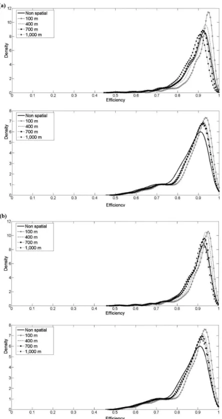
Fig. 2(a) shows the distribution of efficiency for irrigated and rainfed farms using non-spatial model and spatial models (at 100, 400, 700, and 1,000 m) in the case of plot neighborhood. Interestingly, in all four scenarios, the distribution is skewed toward the right and has a relatively long left tale. Very few farmers have efficiency levels less than 0.5. The distribution of efficiency varies not only by ecosystem, but also by type of neighborhood. In every case, the distribution of the non-spatial model is very distinct from the non-spatial models. This finding exposes the biases in efficiency levels that arise when spatial considerations are ignored, i.e., cases where the effi-ciency distribution from spatial models is located to the right of the nonspatial efficiency distribution. More specifically, for the case using plot neighborhood, models for irrigated farms where spatial effects were found to be relatively high (100 and 400 m) have a narrow distribution to the right of the nonspa-tial efficiency distribution. This suggests that part of the farm inefficiency not captured under the nonspatial model can be explained by these spatial models. Also, the fact that the dis-tribution shape is narrower indicates that differences between farm efficiency levels have been reduced once spatial effects have been taken into account.
Hence, although we find that the shorter the distance, the greater the spatial dependence in both cases of irrigated and
rainfed, we can see in Fig. 2(a) (bottom) that for rainfed farms the effect of such increase in spatial dependence with dis-tance is relatively small in explaining efficiency (efficiency distributions are closer to each other than for Fig. 2a (top)). Additionally, considering the nonspatial efficiency distribution as a reference, we found that the efficiency distribution using the spatial model for irrigated farms (100 m, 400 m) and rain-fed farms (all distances) is situated to the right of the non-spatial case (Fig. 2a). This means that for irrigated farms, spatial dependence may help explaining inefficiency, i.e., ir-rigated farmers working more closely. However, for rainfed farms, which work more independently but are more affected by climatic conditions, spatial dependence contributes relatively more to explaining efficiency than irrigated farms (i.e. taking the non-spatial distribution as reference the gap to the 100 m distribution to the right is greater for rainfed farms than for irrigated farms).
For irrigated farms, information sharing about technology among plot neighbors may determine production levels. This may not be the case for rainfed farms whose practices may be determined more independently, and the level of production may be more dependent on the plot’s location, i.e., specific agronomic conditions rather than sharing knowledge. When examining spatial models that use large neighborhood areas and their contributions to explaining inefficiency, e.g., compar-ing efficiency distributions uscompar-ing the spatial dependence model (cut-off distance 1,000 m) versus nonspatial dependence model (cut-off distance 100 m) for irrigated farms, we found small spatial dependence in our longer distance spatial model.
Fig. 2(b) shows the distribution of efficiency for irrigated (top) and rainfed (bottom) farms, using a nonspatial model and spatial models (at 100, 400, 700, and 1,000 m) in the case of residential neighborhood structure. For the models on irrigated farms, the same findings were produced as in the case of plot neighborhood, suggesting that both natural con-ditions of the spatial area and communication between farm-ers with neighbor residence plays a role in explaining part of
Fig. 2. (a) Distribution of efficiency in irrigated farms (top) and rainfed farms (bottom) using plot coordinates. (b) Distribution of efficiency in irrigated farms (top) and rainfed farms (bottom) using residence coordinates.
the inefficiency detected by the nonspatial models. As in the plot coordinates case, the efficiency distribution for rainfed farms when spatial effects are taken into account are differ-ent from the efficiency distribution obtained by the nonspatial model.
This aforementioned finding suggests that natural conditions are likely playing a role in explaining the estimated inefficiency levels gathered by the nonspatial model.
Spatial dependence can explain why the level of connect-edness, i.e., working together and sharing information, is
Fig. 3. (a) Percentage change in efficiency score between spatial model (100 m) and nonspatial (plot coordinates). (b) Percentage change in efficiency score between spatial model (100 m) and nonspatial (residence coordinates). [Color figure can be viewed at wileyonlinelibrary.com]
important in explaining efficiency levels. We found that dif-ferent neighborhood (residential and plot) explain similar spa-tial processes, and there are two types of processes that are captured by residential neighborhood and plot neighborhood. Both social and environmental conditions are captured for farm-ers’ residence and plot location. Using plot neighborhood, Fig. 3(a) shows the map of percentage change in farm effi-ciency levels for both irrigated and rainfed farms in this study area. Rainfed farms tend to have greater increases in efficiency levels once the spatial dependency is incorporated into the anal-ysis. Irrigated farms have relatively less increase in efficiency levels once spatial dependency is incorporated.
The finding above needs some clarification because we found stronger spatial dependency in irrigated area. Irrigated farms being more spatially dependent means that the efficiency lev-els of neighboring irrigated farms are more similar between
them than the efficiency levels of neighboring rainfed farms. This is possibly due to conditions and practices under irrigation being more similar between neighboring irrigated farms than the conditions and practices under rainfed between neighboring rainfed farms. The fact that we can capture this with the spa-tial models helps us identify better farm efficiency levels (i.e., avoiding attributing unobservable environmental conditions to inefficiency). The nature of the spatial dependency is what de-termines its effect of spatial dependency on the farm efficiency estimation. Thus, for irrigated farms the nature of spatial de-pendency may come from similar environmental conditions and practices (e.g., through sharing information), whereas for rain-fed farms it may come from more variable conditions (e.g., cli-matic and topographical conditions). Being able to capture un-observable variable conditions was found to be relatively more important in explaining efficiency levels for rainfed farms than
capturing unobservable environmental conditions and practices for explaining farm efficiency levels for irrigated farms (i.e., accounting for more variable conditions such as weather condi-tions are more determinant than more “controlled” condicondi-tions in explaining efficiency levels).
Fig. 3(b) shows the map of percentage change in farm effi-ciency levels for both irrigated and rainfed farms in the study area using residence neighborhood. In this case, we found sim-ilar results as in the plot neighborhood. We found a higher efficiency increase on the rainfed area than on the irrigated area. Again, we expected this result since natural conditions are expected to be more important in explaining efficiency for rainfed farms than for irrigated farms. Still, we find increase in efficiency levels for irrigated farms. This finding may be a result of the residence neighborhood, or it may be a result of partially capturing the social aspect.
The percentage average increase in efficiency is, on average, higher for rainfed farms (3.4% and 3.3% for plot and residential neighborhood) than for irrigated farms (2.9% and 2.6% for plot and residential neighborhood), in light of the average efficiency levels mentioned above for the spatial model using the 100-m cut-off distance for irrigated and rainfed farm (0.91 and 0.88), and the efficiency levels obtained from the equivalent nonspa-tial models (0.89 and 0.85). Hence, we found that although the spatial dependence parameter (ρ) tells us the strength of the spatial dependence, which is generally greater for irrigated than for rainfed farms, such strength, i.e., incorporating spatial dependency into the analysis, follows a nonlinear relationship with how well the spatial model performs compared with the nonspatial model in terms of percentage change in efficiency between spatial and nonspatial models. To explain, using the plot neighborhood structure, the spatial dependence parameter at 100 m for irrigated and rainfed farms is 0.195 and 0.086, respectively, and the percent efficiency increase is 2.6% and 3.3% for irrigated and rainfed farms, respectively.
The estimated models also show noteworthy results. Educa-tionhas a positive and significant effect in irrigated as well as rainfed environments. Even though the rainfed farmers are more educated by about 0.4 years than irrigated farmers, there was no significant difference in means between the two ecosystems (see Table 1). In the irrigated area, the rice farming is more modern-ized in the sense that farmers use new and improved varieties and chemical inputs, as well as following standardized agro-nomic practices under controlled irrigation. Formal education for literacy as well as basic scientific knowledge is important to understand these types of practices. The fact that educa-tion significantly contributed to improve output in the rainfed environment also makes sense because even though farming is less intensified in the rainfed environment; formal educa-tion is still useful to the rainfed farmers. In fact, the results in Table 2 show the largest educational impact in the rainfed farm-ers’ plot neighbor model (0.013). Additionally,Household size
was found to be insignificant in all estimated models. This find-ing was expected because more farmers reach out to hired labor for farm operations. Finally, regarding the dummy variables for
the studied periods we found that results corroborate the ex-pected effects where rice production in periods 2 and 4 levels was lower than the first period (i.e., the benchmark period) due to the severe drought in the second season and flood in the fourth season mentioned above.
6. Conclusions and policy implications
This article investigates the role of spatial dependency in TE for different ecosystems and neighborhood structures focusing on rice farmers in Bohol, Philippines. A spatial econometrics Bayesian approach was used to estimate the stochastic pro-duction parameters, as well as the spatial dependency parame-ters. The results were compared with nonspatial Bayesian SFA. We found that spatial dependency exists at the residential and plot levels, maintaining more strength for irrigated than rainfed farms. We also found that technical inefficiency levels decrease as spatial effects are more taken into account. Since the spatial effects increases with a shorter network distance, the decreasing technical inefficiency means that the unobserved inefficiencies can be explained better by considering small networks of rel-atively close farmers over large networks of distant farmers, reflecting the location-specific nature of farming.
Two policy implications can be drawn from this study. First, a stronger spatial dependency in the irrigated area indicates the existence of stronger externalities; a positive shock on one farmer’s TE improves the TE of the nearby farmers. The exis-tence of externalities may justify public interventions. However, it is important to note that we also found that the size of the spa-tially dependent network is small. Hence, such an externality may be easily internalized through collective actions within the small group. In irrigated area, the water users group may serve as an appropriate unit for this purpose. Although this is an im-portant practical issue, it is beyond the scope of this article and requires future study. Additionally, since the rainfed farming is more individualistic, policies which are targeted to individual farmers are relatively more important, in comparison to the case of irrigated area. Having observed a strong impact of schooling years, educational support or extension may work effectively in improving rainfed farmers’ TE, which is currently lower than the irrigated farmers.
Although our analysis focuses on TE for rice production tech-nology change and scale effect are also relevant aspects to be considered in long-term studies. Our data cover only two years which did not allow for TFP growth and technological progress estimation as done in studies like Coelli et al. (2005) Nin et al. (2003), Singbo and Larue (2016) and Umetsu et al. (2003). In addition, evidence of spatial dependency in technological progress has been largely demonstrated in the economic litera-ture. The role of spatial dependence in technological progress has mainly been stressed in the context of regional productivity (see Benhabib and Spiegel, 1994; Griffith et al., 2004; Nel-son and Phelps, 1966). Similar to the endogenous growth the-ory in economic literature, technological progress varies across
farmers and it depends on farmers’ ability to innovate or use the improved technologies. As we highlighted above, farmers use the technology differently with human capital or the level of education being commonly cited as drivers of technolog-ical progress. In addition, farmers located below the frontier require sufficient social capabilities to allow them to success-fully exploiting the technologies employed by the most efficient farmers.
Acknowledgments
We would like to thank the Japan International Cooperation Agency (JICA) and Japan International Research Center for Agricultural Science (JIRCAS) for their financial support of the survey data collection; Shigeki Yokoyama for co-managing the project; Takuji W. Tsusaka for data analysis; Modesto Mem-breve, Franklyn Fusingan, Cesar Niluag, Baby Descallar, and Felipa Danoso of the National Irrigation Administration for arranging the interviews with farmers; and Pie Moya, Lolit Garcia, Shiela Valencia, Elmer Su˜naz, Edmund Mendez, Evan-geline Austria, Ma. Indira Jose, Neale Paguirigan, Arnel Rala, and Cornelia Garcia for data collection. Authors would like to thank the editor-in-charge and two anonymous reviewers for their helpful comments. Pede’s time on this research was sup-ported by the RICE CGIAR Research Program.
References
Aigner, D., Lovell, C.A.K., Schmidt, P., 1977. Formulation and estimations of stochastic frontier production function models. J. Economet. 6(1), 21–37. Alvarez, A., 2004. Technical efficiency and farm size: A conditional analysis.
Agric. Econ. 30(3), 241–250.
Anselin, L., 1988. Spatial Econometrics: Methods and Models. Kluwer Aca-demic Publishers, Dordrecht, Netherlands.
Areal, F.J., Balcombe, K., Tiffin, R., 2012. Integrating spatial dependence into Stochastic Frontier Analysis. Australian. J. Agr. Resource Econ. 56(4), 21– 541.
Areal, F.J., Riesgo, L., 2014. Farmers’ views on the future of olive farming in Andalusia, Spain. Land Use Policy 36, 543–553.
Balde, B.S., Kobayashi, H., Nohmi, M., Ishida, A., Esham, M., Tolno, E., 2014. An analysis of technical efficiency of mangrove rice production in the Guinean Coastal Area. J. Agr. Sci. 6(8), 179–196.
Battese, G.E., 1997. A note on the estimation of Cobb-Douglas production functions when some explanatory variables have zero values. J. Agr. Econ. 48(1–3), 250–252.
Battese, G.E., Coelli, T.J., 1995. A model for technical inefficiency effects in a Stochastic frontier production function for panel data. Empir. Econ. 20(2), 325–332.
Bell, K.P., Bocksteal, N.E., 2000. Applying the generalized-moments estima-tion approach to spatial problems involving microlevels data. Rev. Econ. Stat. 82(1), 72–82.
Benhabib, J., Spiegel, M., 1994. The role of human capital in economic devel-opment: Evidence from aggregate cross-country data. J Monetary Econ. 34, 143–173.
Bockstael, N.E., 1996. Modeling economics and ecology: The importance of a spatial perspective. Am. J. Agr. Econ. 78(5), 1168–1180.
Coelli, T.J., Battese, G.E., 1996. Identification of factors which influence the tenchnical inefficiency of Indian farmers. Australian. J. Agr. Econ. 40(2), 103–128.
Coelli, T.J., Rao, D.S.P., O’Donnell, C.J. Battese, G.E., 2005. An Introduction to Efficiency and Productivity Analysis, 2nd edition. Springer, New York. Druska, V., Horrace, W.C., 2004. Generalized moments estimation for spatial
panel data: Indonesian rice farming. Am. J. Agr. Econ. 86(1), 185–198. Farrell, M.J., 1957. The measurement of productive efficiency. J. Roy. Stat.
Soc. 120(3), 253–290.
Glass, A.J., Kenjegalieva, K., Paez-Farrell, J., 2013. Productivity growth de-composition using a spatial autoregressive frontier model. Econ. Lett. 119, 291–295.
Glass, A.J., Kenjegalieva, K., Sickles, R.C., 2014. Estimating efficiency spillovers with state level evidence for manufacturing in the US. Econ. Lett. 123, 154–159.
Glass, A., Kenjegalieva, K., Sickles, R.C., 2015. A Spatial autoregres-sive stochastic frontier model for panel data with asymmetric efficiency spillovers. RISE Working Paper.
Griffith, R. S., Redding, J., Van, R., 2004. Mapping the two faces of R&D: Productivity growth in a panel of OECD industries. Rev Econ. Stat. 86, 883–895.
Hastings, W.K. 1970. Monte Carlo sampling methods using Markov chains and their applications. Biometrika 57, 97–109.
Hossain, E., Rahman, Z., 2012. Technical efficiency analysis of rice farmers in Naogaon district: An application of the stochastic frontier approach. J. Econ. Devel. Stud. 1(1), 2–22.
Idiong, I.C., 2007. Estimation of farm level technical efficiency in smallscale swamp rice production in Cross River State of Nigeria: A stochastic frontier approach. World J. Agr. Sci. 3(5), 653–658.
JICA, 2012. Impact Evaluation of Bohol Irrigation Project (Phase2) in the Republic of the Philippines. JICA, Tokyo.
Karagiannis, G., Tzouvelekas, V., 2009. Measuring technical efficiency in the stochastic varying coefficient frontier model. Agric. Econ. 40(4), 389–396. Kelejian, H.H., Prucha, I.R., 1999. A generalized moments estimator for the autoregressive parameter in a spatial model. Int. Econ. Rev. 40(2), 509–533. Kim, C.W., Phippa, T.T., Anselin, L., 2003. Measuring the benefits of air quality improvement: A spatial hedonic approach. J. Environ. Econ. Manage. 45(1), 24–39.
Koop, G., 2003. Bayesian Econometrics. John Wiley & Sons Inc., Chichester, West Sussex, UK.
Koop, G., Steel, M.F.J., 2001. Bayesian analysis of stochastic frontier mod-els. In: Baltagi, B.H. (Eds.), A Companion to Theoretical Econometrics. Blackwell, Malden, MA, USA.
Kumbhakar, G., McGukin, 1991. A generalized production frontier approach for estimating determinants of inefficiency in U.S. dairy farms. J. Bus. Econ. Statist. 9(3), 279–286.
Kumbhakar, S.C., Tsionas, E.G., 2005. Measuring technical and allocative inefficiency in the translog cost system: A Bayesian approach. J. Economet. 126(2), 355–384.
Meeusen, W., Van Den Broeck, J., 1977. Efficiency estimation from Cobb-Douglas production functions with composed error. Int. Econ. Rev. 18(2), 435–444.
Metropolis, N., Rosenbluth, A.W., Rosenbluth, M.N., Teller, A., Teller, E. 1953. Equations of state calculations by fast computing machines. J. Chem. Physics 21, 1087–1092.
Michler, J.D., Shively, G.E., 2014. Land tenure, tenure security and farm effi-ciency: Panel evidence from the Philippines. J. Agr. Econ. 66(1), 155–169. Nelson, R., Phelps, E., 1966. Investment in human, technological diffusion, and
economic growth. Am. Econ. Rev. 56, 65–75.
Nin, A., Arndt, C., Preckel, P., 2003. Is agricultural productivity in developing countries really shrinking? New evidence using a modified nonparametric approach. J. Dev. Econ. 71, 395–415.
Quilty, J.R., McKinley, J., Pede, V.O., Buresh, R.J., Correa Jr., T.Q., Sandro, J.M., 2014. Energy efficiency of rice production in farmers’ fields and in-tensively cropped research fields in the Philippines. Field Crop Res. 168, 8–18.
Roe, B., Irwin, E.G., Sharp, J.S., 2002. Pigs in space: Modeling the spatial structure of hog production in traditional and nontraditional production regions. Am. J. Agr. Econ. 84(2), 259–278.
Schmidt, A.M., Moreira, A.R.B., Helfand, S.M., Fonseca, T.C.O., 2008. Spatial stochastic frontier models: Accounting for unobserved local determinants of inefficiency. J. Productiv. Anal. 31(2), 101–112.
Singbo, A., Larue, B., 2016. Scale economies and the sources of TFP growth of Quebec Dairy farms. Canadian J. Agric. Econ. 64(2), 339–363. Tsionas, E.G., Michaelides, P.G., 2015. A spatial stochastic frontier model with
spillovers: Evidence for Italian regions. Scottish J. Pol. Econ. 63(3), 1–14, https://doi.org/10.1111/sjpe.12081.
Umetsu, C., Lekprichakul, T., Charavorty, U., 2003. Efficiency and technical change in the Philippine rice sector: A Malmquist total factor productivity analysis. Am. J. Agric. Econ. 85(4), 943–963.
Supporting Information
Additional Supporting Information may be found in the online version of this article at the publisher’s website:
Appendix A1:Spatial model with cut-off distance of 100 m.
Appendix A2:Non-spatial model supporting information
![Fig. 1. Location of study sites designated by ecosystem. [Color figure can be viewed at wileyonlinelibrary.com]](https://thumb-us.123doks.com/thumbv2/123dok_us/921706.2619182/3.918.167.796.119.672/location-study-designated-ecosystem-color-figure-viewed-wileyonlinelibrary.webp)