Electrical and Computer Engineering Conference
Papers, Posters and Presentations
Electrical and Computer Engineering
2014
Enumerating Maximal Bicliques from a Large
Graph using MapReduce
Arko Provo Mukherjee
Iowa State University
Srikanta Tirthapura
Iowa State University, [email protected]
Follow this and additional works at:
https://lib.dr.iastate.edu/ece_conf
Part of the
Computer Sciences Commons
, and the
Electrical and Computer Engineering
Commons
This Conference Proceeding is brought to you for free and open access by the Electrical and Computer Engineering at Iowa State University Digital Repository. It has been accepted for inclusion in Electrical and Computer Engineering Conference Papers, Posters and Presentations by an authorized administrator of Iowa State University Digital Repository. For more information, please [email protected].
Recommended Citation
Mukherjee, Arko Provo and Tirthapura, Srikanta, "Enumerating Maximal Bicliques from a Large Graph using MapReduce" (2014).
Electrical and Computer Engineering Conference Papers, Posters and Presentations. 53.
Enumerating Maximal Bicliques from a Large Graph using MapReduce
Abstract
We consider the enumeration of maximal bipartite cliques (bicliques) from a large graph, a task central to
many practical data mining problems in social network analysis and bioinformatics. We present novel parallel
algorithms for the MapReduce platform, and an experimental evaluation using Hadoop MapReduce. Our
algorithm is based on clustering the input graph into smaller sized subgraphs, followed by processing different
subgraphs in parallel. Our algorithm uses two ideas that enable it to scale to large graphs: (1) the redundancy
in work between different subgraph explorations is minimized through a careful pruning of the search space,
and (2) the load on different reducers is balanced through the use of an appropriate total order among the
vertices. Our evaluation shows that the algorithm scales to large graphs with millions of edges and tens of
millions of maximal bicliques. To our knowledge, this is the first work on maximal biclique enumeration for
graphs of this scale.
Keywords
Graph Mining, Maximal Biclique Enumeration, MapReduce, Hadoop, Parallel Algorithm, Biclique
Disciplines
Computer Sciences | Electrical and Computer Engineering
Comments
This is the author's version of the work. It is posted here by permission of ACM for your personal use. Not for
redistribution. The definitive version was published in Mukherjee, Arko Provo, and Srikanta Tirthapura.
"Enumerating Maximal Bicliques from a Large Graph Using MapReduce." In Proceedings of the 2014 IEEE
International Congress on Big Data, pp. 707-716. IEEE Computer Society, 2014. DOI:
10.1109/
BigData.Congress.2014.105
. Posted with permission.
Enumerating Maximal Bicliques from a Large Graph using MapReduce
Arko Provo Mukherjee
Iowa State University, [email protected]
Srikanta Tirthapura
Iowa State University, [email protected]
Abstract—We consider the enumeration of maximal bipartite cliques (bicliques) from a large graph, a task central to many practical data mining problems in social network analysis and bioinformatics. We present novel parallel algorithms for the MapReduce platform, and an experimental evaluation using Hadoop MapReduce.
Our algorithm is based on clustering the input graph into smaller sized subgraphs, followed by processing different subgraphs in parallel. Our algorithm uses two ideas that enable it to scale to large graphs: (1) the redundancy in work between different subgraph explorations is minimized through a careful pruning of the search space, and (2) the load on different reducers is balanced through the use of an appropriate total order among the vertices. Our evaluation shows that the algorithm scales to large graphs with millions of edges and tens of millions of maximal bicliques. To our knowledge, this is the first work on maximal biclique enumeration for graphs of this scale.
Keywords-Graph Mining; Maximal Biclique Enumeration; MapReduce; Hadoop; Parallel Algorithm; Biclique
I. INTRODUCTION
A graph is a natural abstraction to model relationships in data. Today’s interlinked data from sources such as the web and online social networks has led to massive graphs. Finding patterns and insights from such data can often be reduced to mining substructures from massive graphs.
We consider scalable methods for discovering densely connected subgraphs within a large graph. We focus on a fundamental dense substructure called abiclique. A biclique in an undirected graph G = (V, E) is a pair of subsets of vertices L ⊆ V and R ⊆ V such that (1) L and R
are disjoint and (2) there is an edge (u, v)∈ E for every
u ∈ L and v ∈ R. For instance, consider the following graph relevant to an online social network, where there are two types of vertices, users and webpages. There is an edge between a user and a webpage if the user “likes” the webpage on the social network. A biclique in this graph consists of a set of usersU and a set of webpagesW such that every user inU has liked every page inW. Uncovering such a biclique yields a set of users who share a common interest, and is valuable for understanding and predicting the actions of users on this social network. Usually, it is useful to identify maximal bicliques in a graph, which are
The research reported in this papers is partially supported by the HPC equipment purchased through NSF MRI grant number CNS 1229081 and NSF CRI grant number 1205413.
A B C D E X Y Z
< {A,B,C}, {X,Y} > is a biclique, but is not maximal <{A,B,C,D,E}, {X,Y}> is a maximal biclique <{A,B,C,D}, {X,Y,Z}> is a maximal biclique
Figure 1: Maximal Bicliques
those bicliques that are not contained within any other larger bicliques. See Figure 1 for an example.
We consider the problem of enumerating all maximal bicliques from a graph (henceforth referred to as MBE).
Many applications in mining data from the web and online social networks have relied on biclique enumeration on an appropriately defined graph. The analysis of web search queries has considered the “click-through” graph [34], which has two types of vertices, web search queries and web pages. There is an edge from a search query to every page that a user has clicked in response to the search query. MBE was used in clustering queries using the click through graph. MBE has been used in social network analysis, in detection of communities in social networks [12], and in finding antagonistic communities in trust-distrust networks [17]. It has also been applied in detecting communities in the web graph [11, 24].
In bioinformatics, MBE has been used widely in con-struction of the phylogenetic tree of life [6, 25, 33, 21], in discovery and analysis of structure in protein-protein interac-tion networks [3, 26], analysis of gene-phenotype relainterac-tion- relation-ships [32], prediction of miRNA regulatory modules [35], modeling of hot spots at protein interfaces [15], and in analysis of relationships between genotypes, lifestyles, and diseases [20]. Other applications include Learning Context Free Grammars [36], finding correlations in databases [10], data compression [1].
Enumerating all maximal bicliques in a graph is an NP-hard problem [23]. This does not however mean that typical cases are unsolvable. There are output-polynomitime al-gorithms whose runtime is bounded by a polynomial in the number of vertices and the number of maximal bicliques that are output [2]. Thus it is reasonable to expect algorithms for MBE that work on large graphs, as long as the number of maximal bicliques output is not too high.
do not scale to large graphs. In particular, current methods have the following drawbacks. First, most are sequential algorithms that are unable to make use of the power of multiple processors. For handling large graphs, it is impera-tive to have methods that can process a graph in parallel. Next, they have been evaluated only on relatively small graphs of a few thousands of vertices, and have not been shown to scale to large graph sizes. For instance, the popular “consensus” method for biclique enumeration [2] presents experimental data only on graphs of up to 2,000 vertices and other works [14, 16] are also similar.1.
Our goal is to design a parallel method that can enu-merate maximal bicliques in large graphs, with millions of edges and tens of millions of maximal bicliques, and which can scale with the number of processors.
A. Contributions
We present a parallel solution to MBE. At a high level, our solution clusters the input graph into overlapping subgraphs that are typically much smaller than the input graph, and processes these subgraphs in different tasks that are run in parallel. For the above clustering approach to be effective on large graphs, we needed to solve two problems.
The first problem is the overlap in work within different tasks. For biclique enumeration, it is usually not possible to assign disjoint subgraphs to different tasks, and subgraphs assigned to different tasks will overlap, sometimes signifi-cantly. The challenge is to ensure that work done in different tasks should overlap as little as possible with each other. We accomplish this through a careful partitioning of the search space so that even if different tasks are processing overlapping subgraphs, they still explore disjoint portions of the search space.
The second problem is load balancing among different tasks. With a graph analysis task such as biclique enumer-ation, the complexity of different subgraphs varies signifi-cantly, depending on the density of edges in the subgraph. With a naive assignment of subgraphs to tasks, this will lead to a case where most tasks finish quickly, while a few take a long time, leading to a poor parallel performance. We present a solution to keep the load more balanced, using an ordering of vertices, which reduces enumeration load on subgraphs that are dense, and increases the load on subgraphs that are sparse, leading to a better load balance overall.
We also considered another approach to parallel MBE, us-ing a direct parallelization of the “consensus” algorithm [2], which is probably the most commonly used sequential al-gorithm for MBE. We found that this method takes substan-tially greater runtime than our clustering based method. We also consider the related problem of generating only large maximal bicliques, which have at least a certain number
1In our experiments, we show that the consensus method and other
current methods are unable to process our input graphs in a reasonable time
of vertices. Our parallel algorithms can be easily adapted to this case, using appropriate changes to underlying sequential algorithms.
Experiments: We implemented our parallel algorithm
for MBE on the MapReduce framework [5], and present detailed experimental results on real-world and synthetic graphs. Overall, the clustering approach using a sequential algorithm based on depth-first-search, when combined with our pruning and load balancing optimizations, performs the best on large graphs. This algorithm can process graphs with millions of edges and tens of millions of maximal bicliques, and can scale out with the cluster size. To our knowledge, these are the largest reported graph instances where bicliques have been successfully enumerated.
B. Prior and Related Work
Alexe et. al[2] present a sequential algorithm for MBE using the “consensus” method. Another technique for MBE is based on a recursive depth first search (DFS) [30, 14, 16]. While [14] presents an approach based on a connection with mining closed patterns in a transactional database, [16] present a more direct algorithm based on depth first search. Our parallel algorithm uses a sequential algorithm for pro-cessing bicliques within each task, and we considered both the consensus and the DFS based algorithms; the DFS-based algorithms ran faster overall, and it was easier to optimize the DFS based methods. Due to space constraints, we omit a description of these sequential methods, for details, please refer to an expanded version of this paper [19].
Another approach to MBE is through a reduction to the problem of enumerating maximal cliques, as described in [8]. Given a graphGon which we need to enumerate max-imal bicliques, a new graphG0 is derived such that through enumerating maximal cliques inG0 using an algorithm such as [28, 29], it is possible to derive the maximal bicliques in
G. However, this approach is not practical for large graphs since in going from G to G0, the number of edges in the graph increases significantly.
To our knowledge, the only prior work on parallel algo-rithms for MBE is by Nataraj and Selvan [22]. However, this work does not explore aspects of load balancing and total work such as we do, and moreover, their evaluations are not for large graphs; the largest graph they have considered has 500 vertices and about 9000 edges.
There is a variant of MBE where we only seek induced
maximal bicliques in a graph. An induced maximal biclique is a maximal biclique which is also an induced subgraph of the original graph. We consider the non-induced version, where the enumerated biclique is not necessarily an induced subgraph. If only induced bicliques are needed, they can be obtained by post-processing the output of our algorithm. Note that for a bipartite graph, every maximal biclique is also an induced maximal biclique.
finding the largest sized biclique within a graph (maximum biclique). There are a few variants of the maximum biclique problem, including maximum edge biclique, which seeks the biclique in the graph with the largest number of edges, and maximum vertex biclique, which seeks a biclique with the largest number of edges; for further details and variants, see [4]. MBE is harder than finding a maximum biclique, since it enumerates all maximal bicliques, including all maximum bicliques.
II. PRELIMINARIES
We present a precise problem definition and briefly review the MapReduce parallel programming model.
Problem Definition: We consider a simple undirected graph G = (V, E) without self-loops or multiple edges, where V is the set of all vertices and E is the set of all edges of the graph. Let n = |V| and m = |E|. Graph
H = (V1, E1) is said to be a sub-graph of graph G if
V1⊂V andE1 ⊂E. H is known as an induced subgraph
ifE1consists of all edges ofGthat connect two vertices in
V1. For vertex u∈V, letη(u)denote the vertices adjacent
to u. For a set of vertices U ⊆ V, let η(U) = S
u∈U η(u). For vertex u∈V andk >0, let ηk(u) denote all vertices
that can be reached from u in k hops. For U ⊆ V, let
ηk(U) = S
u∈U
ηk(u). We callηk(U)as thek-neighborhood
of U. For a set of verticesU ⊆V, letΓ(U) = T
u∈U η(u). AbicliqueB =hL, Riis a subgraph ofGcontaining two non-empty and disjoint vertex sets,LandRsuch that for any two verticesu∈Landv∈R, there is an edge(u, v)∈E. A bicliqueM =hL, RiinGis said to be a maximal biclique if there is no other bicliqueM0=hL0, R0i 6=hL, Risuch that
L ⊂L0 andR ⊂ R0. The Maximal Biclique Enumeration Problem (MBE) is to enumerate all maximal bicliques inG.
MapReduce [5] is a popular framework for processing large data sets on a cluster of commodity hardware. A MapReduce program is written through specifying map and reduce functions. The map function takes as input a key-value pair hk, vi and emits zero, one, or more new key-value pairs hk0, v0i. All tuples with the same value of the key are grouped together and passed to a reduce function, which processes a key k and all values associated with k, and outputs a final list of key-value pairs. The outputs of one MapReduce round can be the input to the next round. Further details and examples of use are available in [5, 9]. We used Hadoop [31], an open source implementation of MapReduce, on top of a distributed file system HDFS [27]. While we evaluated an implementation on top of MapReduce, the idea in our parallel algorithm is more generally applicable and can easily be adapted to other frameworks such as Pregel [18].
III. PARALLELALGORITHMS FORMBE
We describe our parallel algorithms for MBE, and give an outline of how these are implemented using MapReduce.
We first present a basic clustering approach, which can be used with any sequential algorithm for MBE, followed by enhancements to the basic clustering approach. We present results about the performance and correctness of our algo-rithms, but omit most proofs due to space constraints.
Basic Clustering Approach: For each v ∈ V, let subgraph (cluster) C(v)be defined as the induced subgraph on all vertices in η2(v)(i.e. the 2-neighborhood ofv inG).
We first note the following.
Lemma 1. Each maximal biclique B in G = (V, E) is a
maximal biclique inC(v)for every vertexvthat is contained inB. Further, for anyv∈V, each maximal biclique inC(v)
is also a maximal biclique inG.
Proof: We show the following two properties. First, every maximal biclique in G must be output as a maximal biclique from cluster C(v) for some v ∈ V. Second, every maximal biclique output from each cluster must be a maximal biclique inG. To prove the first direction, consider a maximal bicliqueM =hL, RiinG. Letv be the smallest vertex in M in lexicographic order, and without loss of generality suppose that v ∈ L. By the definition of a biclique, for each u∈ R, u is a neighbor of v. Similarly, every vertexw∈Lis a neighbor ofv, and is hence inη2(v).
HenceM is completely contained inC(v). Note thatM is also a maximal biclique inC(v). To see this, note that ifM
is not maximal biclique inC(v), thenM is not maximal in
Geither.
We prove by contradiction that every maximal biclique in each cluster C(v) is also a maximal biclique in G. Consider a biclique M emitted as maximal from cluster
C(v) such that it is not maximal in G. Then, there exists a maximal bicliqueM0 that can be generated by extending
M. However, it is easy to see that every vertex inM0 must also be contained inη2(v), and hence M0 is also contained
inC(v), contradicting our assumption thatM is a maximal biclique inC(v).
With the above observation, a basic parallel algorithm for MBE first constructs the different clusters {C(v)|v ∈ V}, and then enumerates the maximal bicliques in the different clusters in parallel, using a sequential algorithm for MBE for enumerating the bicliques within each cluster.
While each maximal biclique in Gis indeed enumerated by the above approach, the same biclique may be enumer-ated multiple times. To suppress duplicates, the following strategy is used: a maximal biclique B arising from cluster
C(v) is emitted only if v is the smallest vertex in B
according to a lexicographic total order on the vertices. The basic clustering framework is generic and can be used with any sequential algorithm for MBE. We have used a variant of the DFS-based sequential algorithm due to [16], as well as the sequential consensus algorithm due to [2]. We call the above basic clustering algorithm using DFS-based sequential algorithm as “CDFS”.
Lemma 2. The basic clustering approach enumerates every maximal bicliques in graphG= (V, E)exactly once.
For an implementation on Hadoop MapReduce, we as-sume that the graph is presented as a file in HDFS organized as a list of edges with each line in the file containing one edge. We generate the cluster C(v) for each vertex using two rounds of MapReduce. The reducer for vertexv in the second round has the clusterC(v), and processes this using a sequential algorithm as described above. Further details can be found in the Technical Report [19].
There are two significant problems with the basic clus-tering approach described above. First is redundant work. Although each maximal biclique inGis emitted only once, through suppressing duplicate output, it will still be gen-erated multiple times, in different clusters. This redundant work significantly adds to the runtime of the algorithm. Second is an uneven distribution of load among different subproblems. The load on subproblemC(v)depends on two factors, the complexity of clusterC(v)(i.e. the number and size of maximal bicliques within C(v)) and the position of
v in the total order of the vertices. The earlierv appears in the total order, the greater is the likelihood that a maximum biclique in C(v) has v has its smallest vertex, and hence the greater is the responsibility for emitting bicliques that are maximal within C(v). A lexicographic ordering of the vertices will lead to a significantly increased workload for clustersC(v)where v appears early in the total order and a correspondingly low workload for clustersC(v) wherev
occurs earlier in the total order.
A. Reducing Redundant Work
In order to reduce the redundant work at different clusters, we modify the sequential DFS algorithm that is executed at each reducer. Algorithm 1 shows the modified DFS Algorithm. The basic observation here is that in cluster
C(v), only those maximal bicliques need be enumerated for whichvis the smallest vertex. As shown in Algorithm 1, we use this observation to prune the search space at the reducer. We call the above DFS based clustering algorithm, with the pruning optimization as “CD0”. Due to space constraints, we omit the details of the entire algorithm description, which, along with all proofs of correctness can be found in our technical report [19].
B. Load Balancing
In Algorithm CD0, vertices were ordered using a lexi-cographic ordering, which is agnostic of the properties of the cluster C(v). The way the optimized DFS algorithm works, the enumeration load on a clusterC(v)depends on the number of maximal bicliques within this cluster as well as the position of v within the total order. The earlier that
v is in the total order, the greater is the load on the reducer handling C(v).
Algorithm 1: Optimized DFS – CD0 Seq(G0, X, T,
key,s)
Input: G0,X,T,key,s
1 forall the vertexv∈T do 2 if |Γ(X∪ {v})|< sthen
3 T ←T\ {v}
4 if |X|+|T|< sthen
5 return
6 Sort vertices in T as per ascending order of
|Γ(X∪ {v})|
7 forall the vertexv∈T do
8 T ←T\ {v}
9 if |X∪ {v}|+|T| ≥s then
10 N ←Γ(X∪ {v})
11 Y ←Γ(N)
12 if Y contains vertices smaller than keythen
13 continue 14 BicliqueB ← hY, Ni 15 if (Y \(X∪ {v}))⊆T then 16 if |Y| ≥sthen 17 vs←Smallest vertex in B 18 if vs=key then 19 // Maximal biclique found
20 Emit (key←∅,value←B) 21 CD0 Seq(G0,Y,T \Y,key,s)
For improving load balance, our idea is to adjust the position of vertex v in the total order according to the properties of its clusterC(v). Intuitively, the more complex clusterC(v)is (i.e. more and larger the maximal bicliques), the higher should be position ofv in the total order, so that the burden on the reducer handlingC(v)is reduced. While it is hard to compute (or even accurately estimate) the number of maximal bicliques inC(v), we consider two properties of vertexvthat are simpler to estimate, to determine the relative ordering of vin the total order: (1) Size of 1-neighborhood of v (Degree), and (2) Size of 2-neighborhood of v.
Intuitively, we can expect that vertices with higher degrees are potentially part of a denser part of the graph and are contained within a greater number of maximal bicliques. The size of the 2-neighborhood is also the number of vertices in
C(v)and may provide a better estimate of the complexity of handling C(v), but this is more expensive to compute than the size of the 1-neighborhood of the vertex.
The discussion below is generic and holds for both approaches to load balancing. To run the load balanced version of DFS, the reducer running the sequential algorithm must now have the following information for the vertex (key
of the reducer) : (1) 2-neighborhood induced subgraph, and (2) vertex property for every vertex in the 2-neighborhood induced subgraph, where “vertex property” is the property used to determine the total order, be it the degree of the vertex or the size of the 2-neighborhood. The second piece of information is required to compute the new vertex ordering. However, the reducer of the second round does not have this information for every vertex inC(v), and a third round of MapReduce is needed to disseminate this information among all reducers. Further details as well as descriptions of algorithms are presented in the Technical Report [19]. We call the Algorithm using the size of 1–neighborhood of a vertexv as the heuristic as CD1 and the one using the size of 2–neighborhood as CD2.
C. Communication Complexity
We consider the communication complexity of Algo-rithms CD0, CD1 and CD2. For input graph G = (V, E), letm=|E|,∆ denote the largest degree andβ denote the output size (i.e. the sum of the sizes of all the bicliques that are output). The communication complexity of a MapReduce Algorithm is defined as the sum of the total number of bytes emitted by all Mappers and the total number of bytes emitted by all the Reducers. We consider the output size for reducers as contributing the communication complexity since each reducer writes into the distributed le system, thus incurring communication. For a multi-round MapReduce algorithm, the communication complexity is the sum of the complexities over all the rounds.
Lemma 3. Total communication complexity of Algorithm
CD1 / CD2 is O(m·∆ +β).
IV. EXPERIMENTALRESULTS
We implemented our parallel algorithms on a Hadoop cluster, using both real-world and synthetic datasets. The cluster has 28 nodes, each with a quad-core AMD Opteron processor with 8GB of RAM. All programs were written using Java version 1.5.0 with 2GB of heap space, and the Hadoop version used was 0.20.203.
We implemented the DFS based algorithms CDFS (clus-tering DFS with no optimizations), CDO (clus(clus-tering DFS with the pruning optimization), CD1 (clustering DFS with pruning and load balancing using degree), and CD2 (clus-tering DFS with pruning and load balancing using size of 2-neighborhood).
We also implemented the sequential DFS algorithm [16], and the sequential consensus algorithm (MICA) [2]. The se-quential algorithms were not implemented on top of Hadoop and hence had no associated Hadoop overhead in their runtime. But on the real-world graphs that we considered, the sequential algorithms did not complete within 12 hours, except for the p2p-Gnutella09 graph. In addition, we imple-mented the parallel clustering algorithm using the consensus-based sequential algorithm, and we also implemented an
alternate parallel implementation of the consensus algorithm that was not based on the clustering method.
0 2000 4000 6000 8000 10000 0 10 20 30 40 50 60 70 80 Runtime (seconds) # Reducers email-EuAll-0.6 com-DBLP-0.6 ego-Facebook-0.6 (a) Algorithm CD1 0 2000 4000 6000 8000 10000 0 10 20 30 40 50 60 70 80 Runtime (seconds) # Reducers email-EuAll-0.6 com-DBLP-0.6 ego-Facebook-0.6 (b) Algorithm CD2
Figure 3: Runtime versus Number of Reducers.
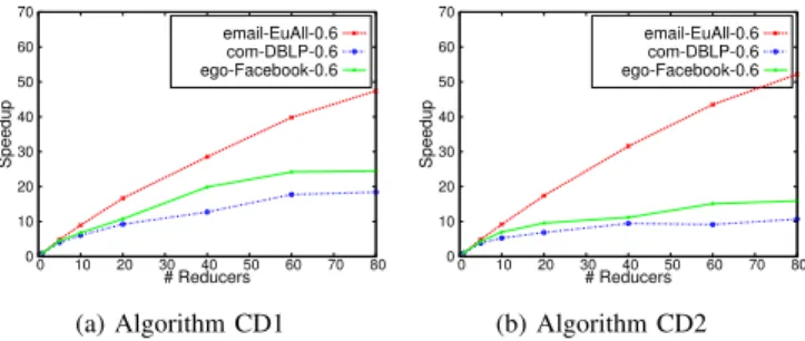
0 10 20 30 40 50 60 70 0 10 20 30 40 50 60 70 80 Speedup # Reducers email-EuAll-0.6 com-DBLP-0.6 ego-Facebook-0.6 (a) Algorithm CD1 0 10 20 30 40 50 60 70 0 10 20 30 40 50 60 70 80 Speedup # Reducers email-EuAll-0.6 com-DBLP-0.6 ego-Facebook-0.6 (b) Algorithm CD2
Figure 4: Speedup versus Number of Reducers. We used both synthetic and real-world graphs. A summary of all the graphs used is shown in Table I. The real-world graphs were obtained from the SNAP collection of large networks [13] and were drawn from social networks, collaboration networks, communication networks, product co-purchasing networks, and internet peer-to-peer networks. Some of the real world networks were so large and dense that no algorithm was able to process them. For such graphs, we thinned them down by deleting edges with a certain probability. This makes the graphs less dense, yet preserves some of the structure of the real-world graph. We show the edge deletion probability in the name of the network. For example, graph GrQc-0.4” is obtained from “ca-GrQc” by deleting each edge with probability0.4. Synthetic graphs are either random graphs obtained by the Erdos-Renyi model [7], or random bipartite graphs obtained using a similar model. To generate a bipartite graph with n1 and
n2 vertices respectively in the two partitions, we randomly
assign an edge between each vertex in the left partition to each vertex in the right partition. A random Erdos-Renyi graph on n vertices is named “ER-hni”, and a random bipartite graph withn1andn2vertices in the bipartitions is
called “Bipartite-hn1i-hn2i”.
We seek to answer the following questions from the experiments: (1) What is the relative performance of the different methods for MBE? (2) How do these methods scale with increasing number of reducers? and (3) How does the runtime depend on the input size and the output size?
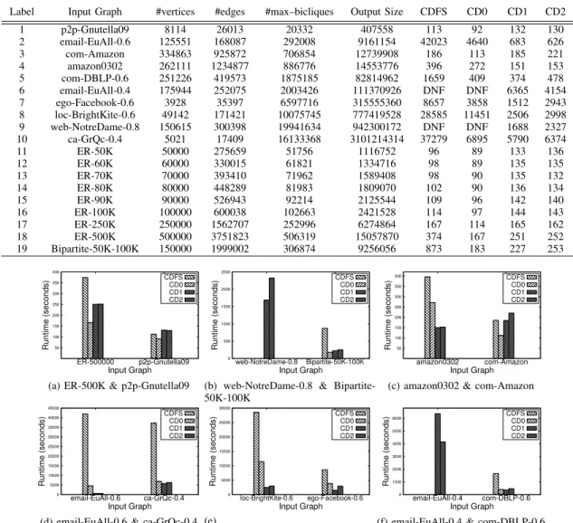
Figure 2 presents a summary of the runtime data for the algorithms in Table I. All data used for these plots was
Table I: Various properties of the input graphs used, and runtime (in seconds) of different algorithms to enumerate all maximal bicliques within the graph using 100 reducers. DNF means that the algorithm did not finish in 12 hours. The size threshold was set as1 to enumerate all maximal bicliques. Runtime includes overhead of all MapReduce rounds including graph clustering, i.e. formation of 2–neighborhood.
Label Input Graph #vertices #edges #max–bicliques Output Size CDFS CD0 CD1 CD2
1 p2p-Gnutella09 8114 26013 20332 407558 113 92 132 130 2 email-EuAll-0.6 125551 168087 292008 9161154 42023 4640 683 626 3 com-Amazon 334863 925872 706854 12739908 186 113 185 221 4 amazon0302 262111 1234877 886776 14553776 396 272 151 153 5 com-DBLP-0.6 251226 419573 1875185 82814962 1659 409 374 478 6 email-EuAll-0.4 175944 252075 2003426 111370926 DNF DNF 6365 4154 7 ego-Facebook-0.6 3928 35397 6597716 315555360 8657 3858 1512 2943 8 loc-BrightKite-0.6 49142 171421 10075745 777419528 28585 11451 2506 2998 9 web-NotreDame-0.8 150615 300398 19941634 942300172 DNF DNF 1688 2327 10 ca-GrQc-0.4 5021 17409 16133368 3101214314 37279 6895 5790 6374 11 ER-50K 50000 275659 51756 1116752 96 89 133 136 12 ER-60K 60000 330015 61821 1334716 98 89 135 135 13 ER-70K 70000 393410 71962 1589408 98 90 135 132 14 ER-80K 80000 448289 81983 1809070 102 90 136 134 15 ER-90K 90000 526943 92214 2125544 109 96 142 140 16 ER-100K 100000 600038 102663 2421528 114 97 144 143 17 ER-250K 250000 1562707 252996 6274864 167 114 165 162 18 ER-500K 500000 3751823 506319 15057870 374 167 251 252 19 Bipartite-50K-100K 150000 1999002 306874 9256056 873 183 227 253 50 100 150 200 250 300 350 400 ER-500000 p2p-Gnutella09 Runtime (seconds) Input Graph CDFS CD0 CD1 CD2
(a) ER-500K & p2p-Gnutella09
0 500 1000 1500 2000 2500 web-NotreDame-0.8 Bipartite-50K-100K Runtime (seconds) Input Graph CDFS CD0 CD1 CD2
(b) web-NotreDame-0.8 & Bipartite-50K-100K 50 100 150 200 250 300 350 400 amazon0302 com-Amazon Runtime (seconds) Input Graph CDFS CD0 CD1 CD2
(c) amazon0302 & com-Amazon
0 5000 10000 15000 20000 25000 30000 35000 40000 45000 email-EuAll-0.6 ca-GrQc-0.4 Runtime (seconds) Input Graph CDFS CD0 CD1 CD2
(d) email-EuAll-0.6 & ca-GrQc-0.4
0 5000 10000 15000 20000 25000 30000 loc-BrightKite-0.6 ego-Facebook-0.6 Runtime (seconds) Input Graph CDFS CD0 CD1 CD2 (e)
loc-BrightKite-0.6 & ego-Facebook-0.6
0 1000 2000 3000 4000 5000 6000 email-EuAll-0.4 com-DBLP-0.6 Runtime (seconds) Input Graph CDFS CD0 CD1 CD2
(f) email-EuAll-0.4 & com-DBLP-0.6
Figure 2: Runtime in seconds of parallel algorithms on real and random graphs. If an algorithm failed to complete in 12 hours the result is not shown. All algorithms were run using 100 reducers. Runtime includes overhead of all MapReduce rounds including graph clustering, i.e. formation of 2–neighborhood.
generated with 100 reducers. The runtime data given for the Parallel Algorithms include the time required to run all MapReduce rounds including time required to construct 2– neighborhood etc.
Inpact of the Pruning Optimization. From Figure 2,
we can see that the optimizations to basic DFS clustering through eliminating redundant work make a significant im-pact to the runtime for all input graphs. For instance, in Figure 2d, on input graph email–EuAll–0.6 CD0, which incorporates these optimizations, runs 9 times faster than CDFS, the basic clustering approach without reducing re-dundant work.
Impact of Load Balancing. From Figure 2, we also
observe that for graphs on which the algorithms do not finish very quickly (within 200 seconds), load balancing helps significantly. In Figure 2d, for graph email–EuAll– 0.6, the Load Balancing approaches (CD1 and CD2) are 7 to 7.4 times faster than CD0, which incorporates the pruning optimization, without load balancing. In Figure 2e, we note that for input graph loc–BrightKite–0.6, CD1 was 4.5 times faster than CD0 and CD2 was about 3.8 times faster. For some graphs, such as email-EuAll-0.4 and web-NotreDame-0.8, CD0 failed to complete even after 12 hours, but CD1 and CD2 completed in less than 2 hours.
For most input graphs, the versions optimized through both load balancing and pruning worked the best overall,
and both these optimizations helped significantly in reducing the runtime.
However, for graphs that completed quickly, load bal-ancing performs slightly slower than CD0 (see Figure 2a). This can be explained by the additional overhead of load balancing (an extra round of MapReduce), which does not payoff unless the work done at the DFS step is significant. Among the two different approaches to load balancing, one based on the vertex degree and the other on the size of the 2-neighborhood of the vertex. From Figure 2 we observed that no one approach was consistently better than the other, and the performance of the two were close to each other. For some input graphs, like Email-EuAll-0.4, the 2-neighborhood approach (CD2) fared better than the degree approach (CD1), whereas for some other input graphs like web-NotreDame-0.8, the degree approach fared better.
To better understand the impact of load balancing, we calculated the mean and the standard deviation of the run time of each of the 100 reducers for the last round of MapReduce of CD0, CD1 and CD2. We present results of this analysis for input graphs loc-BrightKite-0.6 and ego-Facebook-0.6 in Table II. The load balanced algorithms CD1 and CD2 have a much smaller standard deviation for reducer runtimes than CD0.
Consensus versus Depth First Search. Though the
results are not shown here, we note that the consensus algorithm performed very poorly compared with the DFS based algorithm. In all instances except for very small input graphs, clustering using consensus was 6-11 times slower than CD1 and CD2 or worse, and in many cases, clustering consensus did not finish within 12 hours while CD1 and CD2 finished within 1-2 hours. Further, direct parallel consensus, which uses a different parallelization strategy was 13 to 100 times slower than clustering consensus. Further details can be found in [19].
Scaling with Number of Reducers.In Figure 3 we plot the runtime of CD1 and CD2 with increasing number of reducers. In Figure 4, we also plot the speedup, defined as the ratio of the time taken with1reducer to the time taken with r reducers, as a function of the number of reducers
r. We observe that the runtime decreases with increasing number of reducers, and further, the algorithms achieve near-linear speedup with the number of reducers. This data shows that the algorithms are scalable and may be used with larger clusters as well.
Relationship to Output Size. We observed the change in runtime of the algorithms with respect to the output size. We define the output size of the problem as the sum of the number of edges for all enumerated maximal bicliques. Figure 5 shows the runtime of algorithms CD0, CD1, and CD2 as a function of the output size. This data is only constructed for random graphs, where the different graphs considered are generated using the same model, and hence have very similar structure. We observe that the runtime
0 50 100 150 200 250 300 350
0 2e+06 4e+06 6e+06 8e+06 1e+07 1.2e+07 1.4e+07 1.6e+07
Runtime (seconds)
Output Size CD0 CD1 CD2
Figure 5: Runtime versus Output Size for random graphs. All Erdos-Renyi random graphs were used. Output size is defined as the number of edges summed over all maximal bicliques enumerated.
increases almost linearly with the output size for all three
algorithms CD0, CD1, and CD2.
With real world graphs, this comparison does not seem as appropriate, since the different real worlds graphs have completely different structures; however, we observed that the runtimes of Algorithms CD1 and CD2 are well correlated with the output size, even on real world graphs.
0 1000 2000 3000 4000 5000 6000 email-EuAll-0.4 loc-BrightKite-0.6 Runtime (seconds) Input Graph s=1 s=2 s=3 s=4 s=5 (a)
email-EuAll-0.4 & loc-BrightKite-0.6
0 200 400 600 800 1000 1200 1400 1600 1800 web-NorteDame-0.8 ego-Facebook-0.6 Runtime (seconds) Input Graph s=1 s=2 s=3 s=4 s=5 (b)
web-NotreDame-0.8 & ego-Facebook-0.6
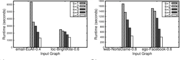
Figure 6: Runtime vs the size threshold for the emitted maximal bicliques. All experiments were performed using Algorithm CD1 and with 100 reducers.
Large Maximal Bicliques. Finally, we considered the variant where only large bicliques, whose total number of vertices is at least s, are required to be emitted. Figure 6 shows the runtime as the size threshold svaries from 1 to 5. We observe that the runtime decreases significantly as the threshold increases.
V. CONCLUSION
Maximal biclique enumeration is a fundamental tool in uncovering dense relationships within graphical data. We presented a scalable parallel method for mining maximal bicliques from a large graph. Our method uses a basic clus-tering framework for parallelizing the enumeration, followed by two optimizations, one for reducing redundant work, and another for improving load balance. Experimental results using MapReduce show that the algorithms are effective in handling large graphs, and scale with increasing number of reducers. To our knowledge, this is the first work to successfully enumerate bicliques from graphs of this size; previous reported results were mostly sequential methods that worked on much smaller graphs.
Table II: Mean and Standard Deviation computation of all 100 reducer runtimes for Algorithms CD0, CD1 and CD2. The analysis is done for the Reducer of the last MapReduce round as it performs the actual Depth First Search.
loc-BrightKite-0.6 CD0 CD1 CD2 Average 1005.94 631.92 625.14 Variance 3470135.82 256859.25 302764.97 Standard Deviation 1862.83 506.81 550.24 ego-Facebook-0.6 CD0 CD1 CD2 Average 479.37 380.32 422.7 Variance 473875.57.82 80146.79 273575.95 Standard Deviation 688.39 283.10 523.04
The following directions are interesting for exploration (1) How does this approach perform on even larger clusters, and consequently, larger input graphs? What are the bottle-necks here? and (2) Can these be extended to enumerate near-bicliques (quasi-bicliques) from a graph?
REFERENCES
[1] Pankaj K. Agarwal, Noga Alon, Boris Aronov, and Subhash Suri. Can
visibility graphs be represented compactly?Discrete & Computational
Geometry, 12(1):347–365, 1994.
[2] Gabriela Alexe, Sorin Alexe, Yves Crama, Stephan Foldes, Peter L. Hammer, and Bruno Simeone. Consensus algorithms for the
gen-eration of all maximal bicliques. Discrete Applied Mathematics,
145(1):11–21, 2004.
[3] Dongbo Bu, Yi Zhao, Lun Cai, Hong Xue, Xiaopeng Zhu, Hongchao Lu, Jingfen Zhang, Shiwei Sun, Lunjiang Ling, Nan Zhang, Guojie Li, and Runsheng Chen. Topological structure analysis of the protein–
protein interaction network in budding yeast.Nucleic Acids Research,
31(9):2443–2450, 2003.
[4] Milind Dawande, Pinar Keskinocak, Jayashankar M Swaminathan, and Sridhar Tayur. On bipartite and multipartite clique problems. Journal of Algorithms, 41(2):388 – 403, 2001.
[5] Jeffrey Dean and Sanjay Ghemawat. Mapreduce: simplified data
processing on large clusters. Communications of the ACM, 51:107–
113, January 2008.
[6] Amy C Driskell, C´ecile An´e, J Gordon Burleigh, Michelle M
McMa-hon, Brian C O’Meara, and Michael J Sanderson. Prospects for
building the tree of life from large sequence databases. Science,
306(5699):1172–1174, 2004.
[7] P. Erd˝os and A. R´enyi. On random graphs I. Publicationes
Mathematicae Debrecen, 6:290–297, 1959.
[8] Alain G´ely, Lhouari Nourine, and Bachir Sadi. Enumeration aspects
of maximal cliques and bicliques. Discrete Applied Mathematics,
157(7):1447 – 1459, 2009.
[9] Sanjay Ghemawat, Howard Gobioff, and Shun-Tak Leung. The
Google File System. InProceedings of the 19th ACM Symposium on
Operating Systems Principles, SOSP ’03, pages 29–43. ACM, 2003. [10] Christopher Jermaine. Finding the most interesting correlations in a
database: how hard can it be? Information Systems, 30(1):21 – 46,
2005.
[11] Ravi Kumar, Prabhakar Raghavan, Sridhar Rajagopalan, and Andrew
Tomkins. Trawling the web for emerging cyber-communities.
Com-puter networks, 31(11):1481–1493, 1999.
[12] Sune Lehmann, Martin Schwartz, and Lars Kai Hansen. Biclique
communities. Physical Review E, 78:016108, Jul 2008.
[13] J. Leskovec. Stanford large network dataset collection. http://snap. stanford.edu/data/index.html.
[14] Jinyan Li, Guimei Liu, Haiquan Li, and Limsoon Wong. Maximal biclique subgraphs and closed pattern pairs of the adjacency matrix: A
one-to-one correspondence and mining algorithms.IEEE Transactions
on Knowledge and Data Engineering, 19(12):1625–1637, 2007.
[15] Jinyan Li and Qian Liu. ‘double water exclusion’ : a hypothesis
refining the o–ring theory for the hot spots at protein interfaces. Bioinformatics, 25(6):743–750, 2009.
[16] Guimei Liu, Kelvin Sim, and Jinyan Li. Efficient mining of large
maximal bicliques. InData Warehousing and Knowledge Discovery,
volume 4081 ofLecture Notes in Computer Science, pages 437–448.
Springer, 2006.
[17] David Lo, Didi Surian, Kuan Zhang, and Ee-Peng Lim. Mining direct
antagonistic communities in explicit trust networks. InProceedings of
the 20th ACM International Conference on Information and Knowl-edge Management, CIKM ’11, pages 1013–1018. ACM, 2011. [18] Grzegorz Malewicz, Matthew H. Austern, Aart J.C Bik, James C.
Dehnert, Ilan Horn, Naty Leiser, and Grzegorz Czajkowski. Pregel: a
system for large-scale graph processing. InProceedings of the 2010
ACM SIGMOD International Conference on Management of data, SIGMOD ’10, pages 135–146. ACM, 2010.
[19] Arko Mukherjee and Srikanta Tirthapura. Enumerating maximal
bicliques from a large graph using mapreduce. http://arxiv.org/pdf/ 1404.4910v1.pdf.
[20] R. A. Mushlin, A. Kershenbaum, S. T. Gallagher, and T. R. Rebbeck. A graph-theoretical approach for pattern discovery in epidemiological
research.IBM Systems Journal, 46(1):135–149, 2007.
[21] N. Nagarajan and C. Kingsford. Uncovering genomic reassortments
among influenza strains by enumerating maximal bicliques. InIEEE
International Conference on Bioinformatics and Biomedicine, 2008, pages 223–230, 2008.
[22] R. V. Nataraj and S. Selvan. Parallel mining of large maximal
bicliques using order preserving generators. International Journal
of Computing, 8(3):105–113, 2009.
[23] Ren´e Peeters. The maximum edge biclique problem is np-complete. Discrete Applied Mathematics, 131:651–654, September 2003. [24] Jayson E. Rome and Robert M. Haralick. Towards a formal concept
analysis approach to exploring communities on the world wide web. In Formal Concept Analysis, volume 3403 ofLecture Notes in Computer Science, pages 33–48. Springer, 2005.
[25] Michael J Sanderson, Amy C Driskell, Richard H Ree, Oliver
Eulenstein, and Sasha Langley. Obtaining maximal concatenated
phylogenetic data sets from large sequence databases. Molecular
Biology and Evolution, 20(7):1036–1042, 2003.
[26] Regev Schweiger, Michal Linial, and Nathan Linial. Generative prob-abilistic models for protein–protein interaction networks–the biclique
perspective.Bioinformatics, 27(13):i142–i148, 2011.
[27] K. Shvachko, H. Kuang, S. Radia, and R. Chansler. The hadoop
distributed file system. In 2010 IEEE 26th Symposium on Mass
Storage Systems and Technologies (MSST), pages 1 –10, may 2010. [28] Etsuji Tomita, Akira Tanaka, and Haruhisa Takahashi. The worst-case
time complexity for generating all maximal cliques and computational
experiments. Theoretical Computer Science, 363:28–42, October
2006.
[29] Shuji Tsukiyama, Mikio Ide, Hiromu Ariyoshi, and Isao Shirakawa. A new algorithm for generating all the maximal independent sets. SIAM Journal on Computing, 6(3):505–517, 1977.
[30] Takeaki Uno, Masashi Kiyomi, and Hiroki Arimura. Lcm ver.2:
Efficient mining algorithms for frequent/closed/maximal itemsets. InIEEE International Conference Data Mining Workshop Frequent Itenset Miing Implementations (FIMI). IEEE, 2004.
[31] Tom White.Hadoop: The Definitive Guide. O’Reilly Media, Inc., 1st
edition, 2009.
[32] Yang Xiang, Philip R. O. Payne, and Kun Huang. Transactional
database transformation and its application in prioritizing human
disease genes. IEEE/ACM Transactions on Computational Biology
and Bioinformatics, 9(1):294–304, 2012.
[33] Changhui Yan, J Gordon Burleigh, and Oliver Eulenstein. Identifying optimal incomplete phylogenetic data sets from sequence databases. Molecular Phylogenetics and Evolution, 35(3):528–535, 2005.
[34] Jeonghee Yi and Farzin Maghoul. Query clustering using
click-through graph. InProceedings of the 18th international conference
on World wide web, WWW ’09, pages 1055–1056, New York, NY, USA, 2009. ACM.
[35] Sungroh Yoon and Giovanni D. Micheli. Prediction of regulatory
modules comprising micrornas and target genes. Bioinformatics,
21(2):ii93–ii100, 2005.
[36] Ryo Yoshinaka. Towards dual approaches for learning context-free
grammars based on syntactic concept lattices. In Developments
in Language Theory, volume 6795 of Lecture Notes in Computer Science, pages 429–440. Springer Berlin Heidelberg, 2011.