Interactive visual analysis promotes exploration of long-term ecological data

of long-term ecological data

TUANPHAM,1,  JULIAJONES,2RONALD METOYER,1FREDERICKSWANSON,3ANDROBERTPABST4

1

School of Electrical Engineering and Computer Science, Oregon State University, Corvallis, Oregon 97331 USA 2

College of Earth, Ocean, and Atmospheric Sciences, Oregon State University, Corvallis, Oregon 97331 USA 3_{USDA Forest Service, Pacific Northwest Station, Corvallis, Oregon 97331 USA}

4_{Department of Forest Ecosystems and Society, Oregon State University, Corvallis, Oregon 97331 USA}

Citation:Pham, T., J. Jones, R. Metoyer, F. Swanson, and R. Pabst. 2013. Interactive visual analysis promotes exploration of long-term ecological data. Ecosphere 4(9):112. http://dx.doi.org/10.1890/ES13-00121.1

Abstract. Long-term ecological data are crucial in helping ecologists understand ecosystem function and environmental change. Nevertheless, these kinds of data sets are difficult to analyze because they are usually large, multivariate, and spatiotemporal. Although existing analysis tools such as statistical methods and spreadsheet software permit rigorous tests of pre-conceived hypotheses and static charts for simple data exploration, they have limited capacity to provide an overview of the data and to enable ecologists to explore data iteratively, and interactively, before committing to statistical analysis. These issues hinder how ecologists gain knowledge and generate hypotheses from long-term data. We present Ecological Distributions and Trends Explorer(EcoDATE), a web-based, visual-analysis tool that facilitates exploratory analysis of long-term ecological data (i.e., generating hypotheses as opposed to confirming hypotheses). The tool, which is publicly available online, was created and refined through a user-centered design process in which our team of ecologists and visualization researchers collaborated closely. The results of our collaboration were (1) a set of visual representation and interaction techniques well suited to communicating distribution patterns and temporal trends in ecological data sets, and (2) an understanding of processes ecologists use to explore data and generate and test hypotheses. We present three case studies to demonstrate the utility ofEcoDATEand the exploratory analysis processes using long-term data on cone production, stream chemistry, and forest structure collected as part of the H.J. Andrews Experimental Forest (HJA), Long Term Ecological Research (LTER), and US Forest Service Pacific Northwest Research Station programs. We also present results from a survey of 15 participants of a working group at the 2012 LTER All Scientists Meeting that showed that users appreciated the tool for its ease of use, holistic access to large data sets, and interactivity.

Key words: cone production; design study; diversity/distribution; forest structure; information visualization; stream chemistry; temporal trends.

Received22 April 2013; revised 5 July 2013; accepted 9 July 2013; final version received 19 August 2013;published25 September 2013. Corresponding Editor: J. Nippert.

Copyright:Ó2013 Pham et al. This is an open-access article distributed under the terms of the Creative Commons Attribution License, which permits unrestricted use, distribution, and reproduction in any medium, provided the original author and source are credited. http://creativecommons.org/licenses/by/3.0/

 E-mail:[email protected]

I

Facilitated by technological advances, recent decades have witnessed the proliferation of complex and large data sets within many fields

of science. In ecology, observations of long-term change are the key to understanding ecosystem function and environmental change (e.g., Knapp et al. 1998, Bowman and Seastedt 2001, Green-land et al. 2003, Shachak et al. 2004, Magnuson et

al. 2005, Chapin et al. 2006, Havstad et al. 2006, Lauenroth and Burke 2008, Redman and Foster 2008, Brokaw et al. 2012). Many ecologists study population dynamics and associated factors such as dynamics of seed supply (Silvertown 1980). In ecosystem and community ecology, long-term trends in stream water nutrient concentrations and fluxes from watersheds are used to examine ecosystem dynamics, such as retention and flux of nutrients and atmospheric pollutants (Likens and Bormann 1995). Similarly, long-term data on plant succession are used to analyze temporal changes in community composition, structure, biomass and nutrients (e.g., Foster and Aber 2004).

Long-term ecological studies commonly in-volve a variety of data sets and hypotheses, but the analysis usually follows three main steps: (1) collect ecological and hopefully relevant environ-mental data; (2) plot and observe overall distri-butions, temporal trends, and correlation of variables in typical charts such as static histo-grams, line charts, and scatter plots; and (3) use statistical tests to confirm or refute the initial hypotheses. This approach may work well when the number of variables is small and interesting hypotheses can be preconceived. However, when the number of variables is large, multiple subsets of data are involved, and/or hypotheses are not well pre-established, moving between static charts and statistical tests (often in different software packages) can become unwieldy, slow, and a limiting method of data exploration. Furthermore, when data sets span many decades, it is likely that the hypotheses and objectives under which a study began evolve as a result of unforeseen trends as well as changes in the knowledge and perceptions of the scientists who work with or inherit the data and experiments. Thus, exploration of new or alternative

hypoth-eses is an inherent part of long-term studies. By data exploration, we mean getting acquainted with data, detecting and describing patterns, trends, and relationships in the data while incorporating the user’s wisdom, knowledge, and intuition (Tukey 1977, Andrienko and Andrienko 2006). In other words, the exploration process usually involves hypothesis generation as opposed to hypothesis testing, decision-mak-ing, scientific modeldecision-mak-ing, or theory development.

Interactive visualizations of data, when com-bined with traditional analysis approaches, offer the potential to facilitate exploratory data anal-ysis, provided that the charts and interactivity fulfill the analytical needs of ecologists and are well suited to characteristics of long-term data. Such an interactive visualization would serve as aneffective user interface for ecologists to explore data directly, formulate and refine hypotheses, and discuss their findings with others, prior to further statistical analysis (Fig. 1). Such a tool would be also useful for quickly detecting erroneous or missing values in the data as part of the data cleansing process. In addition, it is often much easier to detect outliers during the data cleansing process by inspecting the data in a visual representation as opposed to a tabular form (Anscombe 1973). Nevertheless, while typical static charts such as histograms, scatter plots, and line charts have been used by scientists to explore distribution patterns and temporal trends in individual variables, little work has been done to develop interactive visual-analysis tools that support rapid exploration of large, multivariate, and long-term data. The paucity of tools also hinders understanding of potentially different strategies and processes whereby scien-tists gain knowledge and generate hypotheses from long-term data.

We have developed the Ecological Distributions Fig. 1. The visualization driven exploratory analysis process theEcoDATEtool aims to support. Each rectangle represents a subprocess and each arrow represents a direction the user can take to go through the process.

and Trends Explorer (EcoDATE), a web-based visual-analysis tool that facilitates the collabora-tive visual inspection of the distribution patterns and temporal trends of long-term ecological data (Fig. 2). It was refined and evaluated using the user-centered design approach (Shneiderman and Plaisant 2006, Rogers et al. 2007) in which ecologists worked closely with visualization researchers during all stages of the development process from assessing analytical needs to test-ing. The tool, which is readily available at http:// purl.oclc.org/ecodate, supports multiple chart views and a wide range of interaction features involving collaboration among multiple users.

It is important to note thatEcoDATEprovides a means of exploring data using information visualization (InfoVis) rather than the scientific visualization (SciVis) approach. While there is not always a clear boundary between the two fields, they differ in the characteristics of the data analyzed and the corresponding data represen-tations. InfoVis tends to deal with interactive displays of abstract data that do not have natural mappings to 2D or 3D space, such as counts of

insects, cone production, or vegetation cover collected over time (Spence 2007). SciVis con-cerns data that has a natural mapping to two- or three-dimensional space and the visualizations usually involve the physical properties of the data, such as rendering of multiple layers of trees in a forest from LiDAR data (Spence 2007, Cushing et al. 2012).

This paper describes the development and initial application of the tool to three large, long-term data sets: cone production (Jones and Franklin 2012), stream chemistry (Johnson and Fredriksen 2012), and forest structure (Harmon and Franklin 2012) collected as part of the H.J. Andrews Experimental Forest (HJA), Long Term Ecological Research (LTER), and US Forest Service Pacific Northwest Research Station pro-grams. We describe how ecologists have used this tool to overview these datasets, examine and compare distributions and temporal trends, and generate and share hypotheses with others (Fig. 1). We also describe an evaluation of the tool in a working group at the 2012 LTER All-Scientists Meeting (http://asm2012.lternet.edu/).

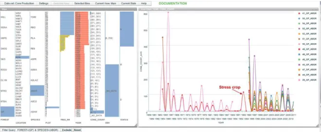
Fig. 2. TheEcoDATEinterface for the cone production data set opened in a browser window. On the left is the multiple histogram view of observations ofAbies grandis trees (grand fir) sampled at Peterson Prairie in the Gifford Pinchot National Forest, Washington, USA. Ecologists used this view (1) to inspect the distributions of this sample with respect to the variables of interest and (2) to generate multiple line series of average cone count over time for multiple sets of trees. The time-series line chart (right view) shows the high degree of synchrony of cone production among 14 individuals ofAbies grandis. It suggests that cone production ofAbies grandisoccurs on a biennial cycle but skipped several years, for example, 1969–1970 and 1972–1973, perhaps due to climate factors. Tree 41 (red line) shows very little cone production from 1973–1992, and then a stress crop in 1993, just before the tree died.

P

C

Here we characterize the analytical needs of ecologists approaching long-term ecological data. These needs are prerequisites for understanding if and how visual analysis can enable insight and discovery.

Long-term ecological research and data

Our study was structured around the central research questions of the HJA LTER program (http://andrewsforest.oregonstate.edu/): (1) how do land use, natural disturbances, and climate affect three key ecosystem properties: carbon and nutrient dynamics, biodiversity, and hydrology and (2) how do these relationships change over time and space? The focus of this work is not to answer these questions but rather to develop a visual-analysis tool to help ecologists approach these questions. To demonstrate the utility of the tool and the data exploration process, we selected three long-term data sets that represent the three major ecological components of biodiversity, carbon, and hydrology.

Cone production data.—Conifer trees commonly dominate the forests in which they occur. Seed production by conifers is not only critical to tree reproduction, but also a vital food resource for many organisms. Since readily-observed cone production is an index of seed production, the history of cone crops gives clues to roles of endogenous (physiological) versus exogenous (climate) factors regulating cone and seed pro-duction. For instance, cone production is known to be cyclical as well as responsive to climate and local environmental conditions (Franklin 1968).

In the Cascade Range of Oregon and

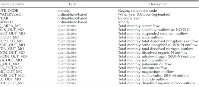
Wash-ington (USA), ecologists have collected data on cone production of upper-slope conifers at 37 locations across 10 national forests every year over a period of 53 years (from 1959 to 2011) (Franklin 1968). The data set has been difficult to analyze because it is large (45,704 observations) and contains many sampled trees (934 distinct trees of 9 species), some of which died or could not be found again, and others were added to replace those lost (Table 1).

Stream chemistry data.—For the past 50 years, small watersheds have been a major setting for ecosystem studies based on long-term records of inputs and outputs (Martin and Harr 1988, 1989, Likens and Bormann 1995). Ecologists have assessed aspects of ecosystem dynamics, such as retention of nutrients and atmospheric pollut-ants in response to natural and management disturbances of vegetation, growth of vegetation, and chemical inputs to the ecosystem. Stream chemistry sampling and analysis was initiated in two small watersheds within HJA in 1968. Over time, sampling expanded to eight gauged water-sheds. Water samples are collected automatically as a function of stage height and flow and composited at stream gauging sites. Analytes include dissolved and particulate nitrogen, phos-phorus, carbon, as well as pH, conductivity, suspended sediment, and a full suite of cations and anions (Table 2).

Forest structure data.—In a study of long-term forest development, ecologists are studying temporal changes in the structure and composi-tion of unmanaged Douglas-fir (Pseudotsuga menziesii) forests (Harmon and Franklin 2012) that established after a stand-replacing wildfire disturbance. The analysis is based on records collected from 21 permanent plots at eight Table 1. Structure of the cone production data set (Jones and Franklin 2012). Each record described by the following variables represents a cone count observation of a particular tree sampled at a particular plot in a particular year. Each plot falls within a location which is situated in a national forest.

Variable name Type Description

SPECIES nominal Species code

TREE_NR nominal Tree number, unique for plot FOREST nominal/spatial National forest code LOCATION nominal/spatial Location code (within forest) PLOT nominal Unique plot number (within location) YEAR ordinal/time-based Sampling year

CONE_COUNT quantitative Number of cones DBH quantitative Diameter at breast height STATUS nominal Status of tree (live, dead, missing)

locations along the Pacific Coast and the Cascade Mountains in western Oregon and Washington. The plots were established between 1910 and 1940, when the forests ranged from 42 to 72 years of age, for the purpose of tracking growth and timber yield of young Douglas-fir forests; in the 1970s forest ecologists began to study forest succession in these plots. Of the 21 plots, 17 are still being measured at regular intervals, provid-ing a data record of up to 100 years on rates of tree growth, trajectories of stand productivity, and the processes and patterns associated with tree mortality, growth, and regeneration. The plots are part of a larger network of long-term plots maintained through the Pacific Northwest Permanent Sample Plot program (PNW-PSP) (Acker et al. 1998) (Table 3).

In summary, long-term ecological data sets are characterized by their large size (thousands of records) and their complexity in terms of the multiple biotic and abiotic variables (e.g., loca-tion, elevaloca-tion, temperature, and rainfall) of varying types (e.g., quantitative, nominal, and ordinal) that are sampled through time. These characteristics—multivariate, geospatial, and connected through time—make them good can-didates for visualization. In this paper, we focus on observational and experimental data and exclude modeled or real-time ecological data (e.g., continuous stream data from sensors).

Visual analytical needs of ecologists

From the information visualization perspec-tive, each of the three long-term ecological data Table 2. Structure of the stream chemistry data set (Johnson and Fredriksen 2012). Each record represents a monthly stream chemistry property collected and aggregated at a particular location in a particular month of a year.

Variable name Type Description

SITE_CODE nominal Gaging station site code WATERYEAR ordinal/time-based Water year (October–September) YEAR ordinal/time-based Calendar year

MONTH ordinal/time-based Month

Q_AREA_MO quantitative Total monthly streamflow

ALK_OUT_MO quantitative Total monthly alkalinity outflow as HCO3-C SSED_OUT_MO quantitative Total monthly suspended sediment outflow SI_OUT_MO quantitative Total monthly silica outflow

TDP_OUT_MO quantitative Total monthly total dissolved phosphorus outflow PO4P_OUT_MO quantitative Total monthly ortho phosphorus (PO4-P) outflow TDN_OUT_MO quantitative Total monthly total dissolved nitrogen outflow DON_OUT_MO quantitative Total monthly dissolved organic N outflow NO3N_OUT_MO quantitative Total monthly nitrate-nitrogen (NO3-N) outflow NA_OUT_MO quantitative Total monthly sodium outflow

K_OUT_MO quantitative Total monthly potassium outflow CA_OUT_MO quantitative Total monthly calcium outflow MG_OUT_MO quantitative Total monthly magnesium outflow

SO4S_OUT_MO quantitative Total monthly sulfate-sulfur (SO4-S) outflow CL_OUT_MO quantitative Total monthly chloride outflow

DOC_OUT_MO quantitative Total monthly dissolved organic carbon outflow

Table 3. Structure of the forest structure data set (Harmon and Franklin 2012). Each record represents an observation of trees in terms of basal area, density, and biomass sampled at a particular location in a particular year.

Variable name Type Description

STANDLOC nominal Stand location

STANDID nominal Stand identifier

AGE ordinal Stand age

SPP nominal Species code

ELEV_M quantitative Elevation (m)

L_BAPH quantitative Basal area of live trees (m2/ha) L_TPH quantitative Density of live trees (no. trees/ha)

sets presents a challenging multivariate visuali-zation problem. Employing the user-centered design approach—which we describe later in the Design and Implementation of EcoDATE section—we have identified the general require-ments for a visual-analysis tool targeting ecolog-ical long-term data with an emphasis on distributions and temporal trends. Specifically, the tool should enable users to do the following: Requirement 1 (R1): distribution patterns.—See and relate distributions of variables simulta-neously and iteratively without making assump-tions about their shapes. In doing so, the tool should also allow users to repetitively filter data to specific subsets and compare them. In addi-tion, the tool should be able to handle large data sets (thousands of records).

Requirement 2 (R2): temporal trends.—See tem-poral trends of variables and compare these trends iteratively across space and species. For example, for the cone production data set, ecologists are interested in the patterns and relative strengths of synchronicity of cone pro-duction across time, space, and species. There-fore, in this example, the tool should enable ecologists to isolate time-series for different sets of trees of interest and to use an appropriate chart that supports time-oriented data to com-pare these series.

Requirement 3 (R3): collaboration.—Keep track of findings at any stage of visualization, share findings with other users, and invite others to build on or modify the visualizations. Scientists and educators may also use the tool to teach students about data exploration in general, and their exploratory process in particular.

Requirement 4 (R4): usability.—Learn to use the tool quickly and easily. From our experience, users of the tool may have varying levels of comfort with computer applications. Therefore, the tool should be simple and easy to use.

E

V

S

The design of theEcoDATEtool was informed by related work on visual representation tech-niques and visual-analysis tools, including those currently employed by ecologists. In this section, we assess their applicability to exploring long-term ecological data, with regards to the four design requirements (R1–R4).

Visual representations for ecologists

A visual representation or chart type deter-mines how data are represented or visualized. Along with interaction features, visual represen-tation techniques serve as the primary compo-nents in visual analysis tools that we assess here. Ecologists typically employ standard 2D/3D displays as classified by Keim (2002). Examples include histograms, boxplots, and scatter plots. They effectively support tasks such as inspecting distributions, outliers, clusters, and correlations over one or two variables (Seo and Shneiderman 2005) (support of R1). Ecologists use rank/ abundance plots (Whittaker 1965) to visualize species abundance and diversity (support of R1). Ecologists commonly represent time series data as a line chart in which time is presented as a linear, ordered x-axis and data cases are plotted by their time values (Aigner et al. 2007) (support of R2). The EcoDATE tool incorporates existing standard displays commonly used by ecologists, such as multiple histograms and time-series line charts, into a user-friendly interface and aug-ments them with appropriate interaction fea-tures.

Visual analysis tools for ecologists

A visual analysis tool facilitates data analysis with visual representations and interactive fea-tures. To the best of our knowledge, little work has been done to develop visual analysis tools specifically for analysis of distributions and temporal trends in long-term ecological data. Here we discuss the merits of four types of tools used by ecologists that contain visual analysis components: (1) widely used software packages such as spreadsheet programs and statistical software packages; (2) specific tools for particular calculations (e.g., estimates of species diversity, calculation of primary productivity); (3) data repositories or portals; and (4) workflow man-agement systems (e.g.,Kepler). O’Donoghue et al. (2010) provide an overview on visualization of biological data.

Ecologists often use charting components in spreadsheets and statistical software packages for visual analysis prior to statistical analyses; these tools permit quick and simple visual inspection and they are easy to learn (support of R4). However, these tools lack interactive capacity, for instance, they do not readily permit

iterative subsetting and replotting of data, which are essential steps in hypothesis formulation (Andrienko and Andrienko 2006) (lack of inter-activity for R1 and R2).

A second group of tools includes software designed for specific types of ecological data analysis, such as estimation of species diversity and abundance (Colwell 2010) or simulation of hydrologic models with input data (Rink et al. 2012). These tools provide rigorous statistical tests and modeling techniques to answer specific scientific questions, for example, what is the species richness of dataset A? Or what data should be used to define parameters for hydro-logic model B? However, these tools do not support exploration of distribution patterns and temporal trends with interactive charts (lack of R1 and R2). Therefore, we do not consider these tools further.

A third type of visual analysis tool is ecological data repositories or portals that support collec-tion, archival, and synthesis of long-term data from multiple sites, for example, EcoTrends (Servilla et al. 2008, Peters et al. 2011) and Clim-DB/Hydro-DB(Henshaw et al. 2006). These web-based portals are usually equipped with static visual representations such as line charts for simple and quick visual exploration of temporal trends in existing long-term data sets (partial support of R2). Although these tools may have limited capacity for subsetting, they are not designed to support distribution patterns in multiple attributes (lack of R1), interaction features (lack of interactivity for R1 and R2), or collaboration features (lack of R3).

A fourth class of software tools for visual analysis is designed to support‘‘workflows,’’i.e., the analysis process of scientists (support of R3), such as Kepler (Luda¨scher et al. 2006) and VisTrails (Callahan et al. 2006). Although these tools are powerful and potentially useful to ecologists, they require customization and pro-gramming to fit the specific analytical needs of ecologists, especially with respect to visual representations and interaction features (lack of R4). Therefore, these tools may be more suitable for information managers who have expertise in managing data in repositories and who help ecologists with data pre-processing tasks such as data gathering and cleansing.

General visualization tools

In addition to tools developed by and for ecologists, a wide range of information visualiza-tion tools is available that, to some extent, meet the design requirements for ecologists (Roberts 2007, Heer and Agrawala 2008, Heer and Shnei-derman 2012). For example, software systems such as Tableau (http://www.tableausoftware. com/) and Spotfire (http://spotfire.tibco.com/) are dedicated visual analysis tools, as distin-guished from charting components in spread-sheet or statistical tools. They provide pre-defined chart types and a variety of controls for interacting with data, for example, to subset data (support of R4). They also support multiple, coordinated views; and users can publish and share visualization dashboards as interactive Web pages (support of R3). However, these applications are not necessarily tailored to specific analytical needs of ecologists (lack of R1 and R2). For example, ecologists may want to discretize quantitative variables interactively to reveal different distribution features of the data (R1). Also, ecologists may want to repeatedly generate subsets of time-series data and plot them in a line chart in order to examine temporal trends (R2).

T

E

DATE T

A visual analysis tool consists of (1) represen-tations (i.e., charts, graphs) and (2) interaction features (i.e., subsetting, bookmarking, etc.). The various types of interaction features can be described using a classification system for visual analysis tasks proposed by Heer and Shneider-man (2012). The classification consists of three high-level categories of task types: a user makes a set of decisions about types of charts and organization of data (data view and specification), how to manipulate the visualization views (view manipulation), and how to reproduce and share the visualizations (process and provenance). The representations and interaction features of Eco-DATE are outlined following this classification system (Table 4) and discussed based on the four design requirements presented earlier (R1–R4).

The EcoDATE interface (Fig. 2) supports multiple views (or windows) each of which can be manipulated (select, drag and drop, resize, and close). While the interface is web-based, its

look and feel is similar to a desktop interface that is familiar to users (support of R4).

Chart types

The current version of EcoDATE (ver. 1.0) supports two widely used chart types: multiple histograms and a line chart. Coordination be-tween views of these chart types loosely follows

the master/slave relationship (Roberts 2007), in which the master views of multiple histograms are used to query/retrieve data and to generate line series for line charts. Other than that, views are independent from each other.

Multiple histograms.—The purpose of this rep-resentation is to show distributions of multiple variables, which permit the user to identify and Table 4. Interaction techniques supported by theEcoDATEtool. Each of the techniques is designed to facilitate specific analytical needs of ecologists. Most of the techniques (if not explicitly noted) are applied to the multiple histogram views. The classification is adapted from Heer and Shneiderman (2012).

High-level

category Task type EcoDATE’s features Specific analytical needs of target users Data and view

specification

Visualize Choose among multiple histograms and line charts

Inspect distributions of variables with multiple histograms and temporal trends with time-series line charts Filter (or Subset) Filter data based on selection of bins Examine different data subsets or

samples of observations Sort/Reorder Sort bins within a variable by names

or by abundances Organize the data according to afamiliar unit of analysis (e.g., rank species from rare to common) Reorder variable axes Group axes by their common or

user-defined characteristics (e.g., group of covariate/response variables) Derive Discretize quantitative variables Experiment with different discretization

settings (e.g., isolate specific range of interest) to reveal different features of the data

Group/ungroup bins within a

variable Group outliers or similar variablevalues to fit users’hypotheses (e.g., group species of the same genus or family)

Scale (normalize) bins’abundances Accommodate data sets with different distributions

View Manipulation Select/Highlight Select or highlight a view, axes, bins, or line series

Select or highlight elements of interest for other operations, such as filter, sort, derive

Navigate Navigate and control views/ windows using the top menu bar and the bottom status bar

Know where and how to navigate views

Coordinate Duplicate multiple histogram views Compare data subsets side-by-side Use multiple histograms as a query

builder to construct series data for line charts

Construct multiple line series and compare them

Organize Open, close, resize, and layout views Manage views for comparison or effective presentation to others Show/hide error bars in line charts Access additional information on

demand Process and

Provenance Record Log user interactions Undo/redo actions, reproduce statesstep-by-step. These features are reserved for future work.

Annotate Color axes and Label line series Distinguish among axes or line series based on their common or user-defined characteristics

Share Bookmark visualization states Revisit/share visualization states with others for collaborative and iterative exploration of data

Export view data Analyze data further with statistical tools

Guide Display data tips for menu bars, axes, bins, and line series

Guide users through menu items and provide additional information on highlighted items

interactively specify subsets of data (support of R1). Like previous work, this multiple histogram representation presents variables in a parallel axis layout (Hauser et al. 2002, Pham et al. 2011). Histograms are placed vertically side-by-side, one histogram for each variable, as opposed to horizontally. In these views, the bars extend to the right (in contrast to the familiar upward-extending display). A vertical arrangement of histograms allows more variables to fit in wide-screen displays and facilitates the placement and reading of labels from left to right, as shown by an example of a subset of the cone production data set (Fig. 2, left view). The ecologist user can duplicate multiple histogram views to compare data subsets side-by-side. Continuous numerical variables are discretized intobinsto plot relative frequency. That is, the length of each bar is scaled according to l(x)¼ jxj/jxMAXj where jxj denotes the number of observations in binx, andxMAXis the bin with the most observations for the variable in question.

Line chart.—The purpose of this representation is (1) to show overall trends in a continuous, real-valued variable, such as cone production or tree density, over the sampling period of interest; and (2) to support comparison of values of the variable at different time points or intervals (support of R2) and across multiple samples. In

line charts, ordinal variables such as time are presented as a linear ordered axis, x-axis, and values at each point in time are plotted along the y-axis. For example, Fig. 2, the right view depicts multiple line series of average cone count over time for multiple sets of trees in the cone production data set. Optionally, users can display error bars as standard errors or standard deviations on the line series (Fig. 3).

Interaction features

The EcoDATE tool supports a wide range of interaction features (Table 4). We extend our description of a subset of prominent features here, emphasizing its utility in the context of the distributions and trends analysis.

Subsetting/filter.—Given an overview of data distribution in multiple histogram views, ecolo-gists often want to shift their focus repetitively among different subsets or samples of observa-tions, for example, to examine distributions of species at different locations. Ecologists also want to generate subsets of data for other representa-tions, such as a line chart. Subsetting or filtering operates on selected bins. A filter ‘status’bar at the bottom will show the filter query for the currently selected view (see Fig. 2). To construct a complex filtering query consisting of multiple bins, we follow a simple and commonly used Fig. 3. Line series of average cone production from Pinus species (pine trees) from 1962–2011 showing a declining trend. Users can select to display error bars as standard errors or standard deviations on the line series. Users can place the mouse pointer over the data points on the line series for additional information.

rule articulated by ecologists: bins within a variable are connected by the ‘‘OR’’ condition, whereas groups of filtered bins across variables are connected by the ‘‘AND’’ condition. For example, the left view of Fig. 2 visualizes a subset of observations filtered by Abies grandis trees (grand fir) AND sampled at Peterson Prairie in the Gifford Pinchot National Forest, Wash-ington, USA (see the bottom bar for the query). Users can also inverse (or exclude) the query to obtain the complement of a subset. To some extent, multiple histogram views can be used to quickly and visually construct a query (as opposed to typing a query command) (support of R1).

Sort/reorder.—Users can sort bins within a variable by names or by abundances (support of R1). The goal is to organize the data according to a familiar unit of analysis, for example, species ranked from rare to common. They can also reorder variable axes according to common or user-defined characteristics of variables. For example, they might group a set of covariate/ response variables or create groups of nominal (e.g., species, habitat), ordinal (e.g., sampling month, year), or quantitative (e.g., cone count, basal area) variables.

Derive.—In many cases, to examine different data distribution settings, ecologists wish to generate derived data such as discretized

quan-titative variables or groups of bins. While they can do so prior to importing data for visual analysis, moving between tools disrupts the flow of the iterative exploration process (Elmqvist et al. 2011). Using EcoDATE, ecologists can discre-tize quantitative variables, based on their knowl-edge of ecology, without leaving the application (support of R1). EcoDATE allows ecologists to flexibly experiment with discretization settings by specifying the range of interest and bin size (see Fig. 4). In addition, for categorical variables, similar to discretization, ecologists can group or ungroup bins within a variable based on their hypotheses (support of R1). For example, they can group species based on their rarity or their functional groups. For example, ecologists ex-ploring the forest structure data set may wish to select and group species such as western hem-lock (Tsuga heterophylla), western redcedar (Thuja plicata), Pacific yew (Taxus brevifolia), and bigleaf maple (Acer macrophyllum) into a group of shade-tolerant species before comparing it to Douglas-fir.

Share.—Collaborators are often geographically dispersed with the physical distance and time differences making collaborative exploration dif-ficult. Using the EcoDATE tool, ecologists can discuss and share findings with collaborators by bookmarking visualization states (e.g., Fig. 2) as unique web URLs (support of R3). These Fig. 4. Discretization settings for variable CONE_COUNT. Ecologists can narrow the range of interest for this variable to [1, 301] and specify a bin size of 10. The result will automatically include two separate out-of-range bins for [0, 1) and [301, 5001) as shown in Fig. 2 (left view, the CONE_COUNT histogram).

bookmarks can be easily shared via email or embedded to the user’s notes, serving as a common ground for discussions among collabo-rators.

The implementation of bookmarking in Eco-DATE stores ‘‘snapshots’’of visualization states (e.g., Fig. 2) including aggregated static data (for bins and line series) as opposed to providing dynamic access to the most current data (Heer et al. 2008b). This implementation decision is based on the understanding of characteristics of large ecological data sets. The data are usually static and the analysis process involves inspecting distributions or trends of observations as aggre-gation of data as opposed to individual data points. BecauseEcoDATEstores only aggregated data, the storage cost is efficient and the loading time of visualization states is fast.

D

I

User-centered design with ecologists

A close collaboration between ecologists and visualization researchers was critical for design and integration of the EcoDATE tool into the ecologists’analysis process. We employed a user-centered design approach, specifically, participa-tory design (Shneiderman and Plaisant 2006, Rogers et al. 2007), in which the ecologists were included as part of the design team. User-centered design is both a philosophy and a process in which the needs, desires, and limita-tions of the target users (e.g., scientists) are considered very closely at every stage of the design process (establishing requirements, de-sign, implementation, evaluation). The process has involved three ecologists and two visualiza-tion researchers, who are co-authors on this paper.

Our participatory design process was iterative, required group design sessions over many weeks, and involved a variety of tools for assessment of user performance and tool usabil-ity such as observations, interviews, log books, and automated logging of user interactions (Shneiderman and Plaisant 2006). In addition, the visualization researchers engaged with the ecologists to the point of becoming assistants in the process of data exploration. We used email communications to share and discuss visualiza-tion state bookmarks. We set up weekly one-hour

meetings between a visualization researcher and an ecologist in the ecologist’s workplace for several months. Finally, during the development process, we also collaborated with information managers, who manage the ecological data repository of the HJA LTER site. They helped clean data, explained the structure of data sets, and gave feedback on theEcoDATEtool.

Implementation

The EcoDATE tool is a web-based database application implemented following the client– server architecture. In this section, we describe the client and server components of the tool and justify our choice of the architecture.

Client.—The client side ofEcoDATE is respon-sible for representing processed data from the server–that is, representing multiple histogram views and line charts, laying out views and menus, and communicating user interactions with the server. We developed the EcoDATE client interface with Flex 3, which is an open-source framework by Adobe for creating Flash rich internet applications.

Server.—Data sets are stored and managed with the MySQL database management system (DBMS). In addition, we rely on the program-ming languages of PHP (Hypertext Preprocessor) and SQL (Structured Query Language) to handle requests from the client. Specifically, the server is responsible for all data-related logic and compu-tation, such as retrieving and manipulating ecological data, building and maintaining data structures of visualization states, and logging interactions. This client-server model was a natural choice considering that most of the ecological data repositories are structured and stored in a DBMS (Henshaw and Spycher 1998). Metadata are another distinctive property of scientific data in general, and ecological data sets in particular. While generated to aid analysis, metadata present another challenge to data visualization. Specifically, the key variables de-scribed in Tables 1, 2, and 3 were supplemented with additional information about the variable such as descriptions of SPECIES or LOCATION. Technically, the metadata tables need to be joined with the primary data table to form the data set for use in theEcoDATEtool.

Our implementation approach can handle large data sets. Feedback on performance from

ecologists indicates that it is highly responsive for all three data sets of interest on a typical desktop PC. From our tests, heavy interactions such as filtering usually respond in a few seconds provided a high-speed internet connection.

E

One of the most effective ways of evaluating an information visualization tool is through long-term case studies of target users exploring real world data sets using the tool (Shneiderman and Plaisant 2006). In this section, we evaluate EcoDATE by three case studies, one for each of the three data sets: cone production, stream chemistry, and forest structure. Further, we discuss the results from the evaluation of the tool during a working group meeting at the LTER All Scientists Meeting in 2012.

The objectives of the case studies are (1) to demonstrate the utility ofEcoDATEfor ecologists and (2) to describe how use of the tool reveals how scientists analyze data, both individually and collaboratively, and provides scientists with hypotheses that can be tested outside the tool (Fig. 1). Each of the case studies involved multiple observations of ecologists (co-authors of this paper) in multiple work sessions in normal environments (i.e., offices) during which they used the EcoDATEtool to explore the three data sets.

Cone production data case study

The primary objective of this case study is to demonstrate the utility ofEcoDATEin terms of its supported visual representations and interaction techniques. The design of EcoDATE followed closely the Visual Information Seeking Mantra, the widely accepted visual design guideline pro-posed by Shneiderman (1996): ‘‘overview first, zoom and filter, then details on demand’’. This mantra suggests that when the user seeks information from a data set, a tool should allow the user to start first with an overview of the entire data set, then to subset the data (filtering and zooming), and ultimately to get additional fine details as needed.

Summary of information needs.—According to the design requirements, the ecologist user was interested in two key aspects of the cone production data set. First, she wanted to see the

overall distribution of samples in time and space (geographic and environmental) and to be able to relate multiple distributions simultaneously and iteratively. Second, she was interested in the patterns and relative strengths of synchronicity of cone production variation across time, space, and species.

Overview.—The initial multiple histogram view helped the ecologist quickly assess the numbers of sampled trees by species and their distribu-tions across locadistribu-tions and years. She also detected that the range for CONE_COUNT (number of cones per tree) was large (0–5000) and its distribution was positively skewed with very few high values. To examine the number of trees that produced no cones (observations with zero cone count), she was able to use the discretization settings (Fig. 4) to derive (Table 4) new bins that displayed the numbers of trees with zero cones (Fig. 2, left view, the CON-E_COUNT axis).

Filtering/subsetting.—After inspecting the over-view, the ecologist focused on a specific location, in this case, the Gifford Pinchot National Forest (GP), Washington, USA. This forest was of interest because of its complex topography and proximity to Mount St. Helens, whose 1980 eruption may have affected cone production history. First, she filtered the data by bin ‘GP’

in the‘FOREST’variable. While she could select and filter multiple bins at once, she preferred first to inspect the distribution of all cone production observations (i.e., all species) in the GP. Then she filtered the data to examine cone production for Abies grandis(grand fir, ABGR) only.Abies grandis was of interest because it is a common species in mixed conifer forest communities. The view of the new subset helped the ecologist discover that the sampling process was not consistent over time: trees were sampled starting in 1963, but because of gradual, cumulative mortality, the sample size declined over time, so new trees were added in 1995 (Fig. 2, left view, the YEAR axis). She was then able to further filter the data to examine cone production in individual trees with long-term cone production records, as well as to examine mortality at tree, plot, species, and regional scales.

Details on demand.—While inspecting the dis-tribution of the subset of interest (cone produc-tion in Abies grandis at the GP), the ecologist

wanted to compare trends of cone production between trees that died and those that were added to replace them. Tree status (health) during the study period was important because tree health, morbidity, and mortality affect cone production. For example, stand-level cone pro-duction may depend on tree-level processes, including stress crops from dying individuals, insect attacks, and partial wind damage. Using EcoDATE, she was able to identify and plot the trees that were sampled for subsets of the record, which produced a visualization of cone produc-tion in trees that died and trees that were added to replace them. Specifically, to identify trees that were not sampled throughout the entire study period, the ecologist sorted trees (i.e., variable TREE_NR) by the numbers of years of observa-tion. After sorting, she selected trees that had less than a certain number of observations (Fig. 2, left view, the TREE_NR axis) and added data for each of the selected trees as a line series into the YEAR-CONE_COUNT line chart (Fig. 2, right view).

The time-series line chart (Fig. 2, right view) helped ecologists quickly formulate hypotheses that the trees of interest produced cones in synchrony (timing and magnitude) on a biennial cycle, but skipped several years, for example, 1969–1970 and 1972–1973, suggesting the hy-pothesis that some external factor or event may have disrupted the biennial cycle. The view also shows multiple trees that were added to the plot in 1995. In addition, the visualization allowed a discovery that trees that died sometimes pro-duced ‘‘stress crops’’ just before dying: tree 41 (red line) shows very little cone production from 1973–1992, and then a stress crop in 1993, just before the tree died. In all, while the ecologist found no evidence of an effect of the 1980 eruption of Mount St. Helens on cone production history, her exploration led to other interesting scientific discoveries that she did not anticipate before using the visualization.

Note that while this sequence of actions demonstrates a single exploration path, the tool supports pursuit of multiple paths simultaneous-ly and iterativesimultaneous-ly. For example, the ecologist repeated the process and retrieved the data subset for all ‘PINUS’or pine trees (Fig. 3). The time-series line chart for this subset revealed a declining trend of average cone production of

Pinus spp. from 1962–2011, suggesting the hypothesis that tree aging, mortality, or expan-sion of influence of a pest/pathogen may be contributing to declining cone production.

Sharing and further analyses.—Satisfied with her findings, the ecologist bookmarked the current state of the visualization (as shown in Fig. 2) as a URL and emailed the link to her collaborators with a description of her findings. She also exported the data subsets and pursued further analysis using existing statistical tools (e.g., Pearson’s correlation test to quantify the correla-tion between multiple line series with respect to sampling years).

Case study summary.—Using EcoDATE, the ecologist became acquainted with the cone production data and the tool and developed a concrete analysis plan, which, to her, had been vague or possibly subconscious before. Specifi-cally, EcoDATE provided a holistic overview of the observations of interest and helped the ecologist build a mental model of how multiple variables were distributed in the entire data set. This model helped the ecologist to formulate actions such as filter/subset queries, and explore the data broadly and deeply.

Stream chemistry data case study

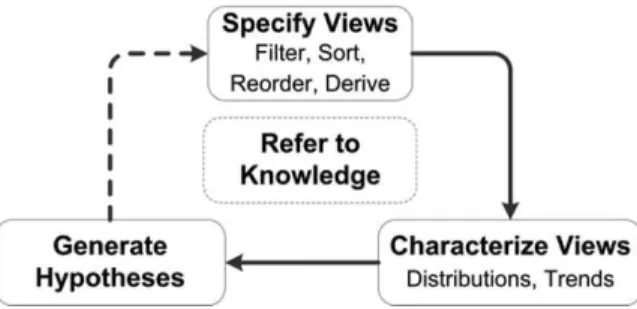
The objective of the next case study is to illustrate the process of using EcoDATE to gain insights into data and to generate hypotheses. Following her experience with EcoDATE and the analysis of the cone production data, the ecolo-gist was more aware of the exploration paths that she would take. From our observations, the ecologist followed a hypothesis generation pro-cess that can be summarized as three main tasks (Fig. 5): (1) specify visualization views(e.g., filter, sort, reorder, derive data), (2) characterize views (e.g., distribution patterns and temporal trends), and (3) gain insights and generate hypotheses. The process is highly iterative with multiple rounds of exploration, guided by discoveries in each round and by the ecological knowledge of the user.

Summary of information needs.—Exploring the stream chemistry data set, the ecologist wanted to investigate distribution and temporal patterns of multiple chemical properties within and across locations (e.g., watersheds) over time, and ulti-mately to make inferences about ecological

processes and events driving these patterns. Before the work sessions, she had examined temporal patterns of stream chemistry using statistical tools. Despite this prior knowledge, the multiple histogram views of the data facilitat-ed by EcoDATE helpfacilitat-ed her generate additional hypotheses based on the shapes of distributions of different chemical constituents. The visualization of the stream chemistry data is available at http:// purl.oclc.org/ecodate/chemistry.

Round 1 of hypothesis generation.—Starting with the default specification of the multiple histogram view (specify), the ecologist quickly noticed (char-acterize) (1) differences in numbers of samples by year and location, (2) differences in the shapes of distributions of the chemical properties over the years and from one property to another, and (3) a relatively large number of extreme values. Using her knowledge, the ecologist related the difference in record lengths (characterization 1) to the hypothesis that sampling must have been turned off and on intentionally at some watersheds (generate hypotheses). To confirm this hypothesis, she planned to access the sampling logs for more information. Further, the characterizations (2) and (3) prompted the ecologist to pursue these paths further, as described next.

Round 2 of hypothesis generation.—To compare the shapes of distributions of the chemical properties, the ecologist first used the discretiza-tion feature (Fig. 4) to specifyequal numbers of bins as well as equal numbers of observations in the extreme value bin (upper range bin) for each of the histograms of the corresponding chemical properties. She then found that distributions

varied among properties in the degree of skew (characterize) (Fig. 6). Specifically, the distribu-tions for silica (SI) and discharge (Q_AREA_MO) were similar to one another and differed from the distributions for nitrate-nitrogen (NO3-N) and suspended sediment (SSED).

From this characterization of the data, the ecologist referred to her knowledge and formu-lated several hypotheses, e.g., (1) extreme suspend-ed ssuspend-ediment output and nitrate-nitrogen output may occur under extreme storm events, when sediment and decomposed litter are entrained; (2) silica output is more dominated by chronic export, which is consistent with its origin from chemical weathering.

Additional rounds of hypothesis generation.— Following up on the hypotheses generated in Round 2, the ecologist rapidly completed addi-tional rounds of exploration. She specified the time-series line charts for the chemical properties of interest to investigate how the extreme values of the properties coincided over time. She subsetted the data to two specific locations (watersheds) and cross-compared their temporal trends of specific chemical properties. After each of the exploration rounds, the ecologist was able to bookmark the visualization state, take snap-shots of the visualization views, and save them along with her notes. In summary, within four one-hour work sessions, the ecologist completed ten rounds of data exploration, generating hypotheses that could be confirmed quickly as well as questions that prompted further analyses (inside or outside of theEcoDATE tool).

Case study summary.—Even though the ecolo-gist had prior knowledge of the stream chemistry data, EcoDATE nevertheless permitted in-depth analysis of the data that led to new insights, especially with respect to specification and characterization of multivariate distribution shapes using the interaction feature of discretiza-tion of bins. Although existing analysis tools such as spreadsheet programs also permit this kind of specification, the process would be cumbersome and time-consuming. We summarized the anal-ysis strategy in this case study as an iterative three-step process of specifying visualization views, characterizing views, and gaining insights while incorporating ecological knowledge and intuition (Fig. 5).

Fig. 5. The iterative process of hypothesis generation supported by EcoDATE. Each rectangle represents a task and each arrow represents a transition from one task to another. The task of involving knowledge in the center supplements all other tasks.

Forest structure data case study

While the stream chemistry case study aims to emphasize the hypothesis generation process supported by EcoDATE, this case study high-lights how EcoDATE helped another ecologist prepare data to upload into EcoDATE, construct the line charts, and gain insights into the forest structure data set.

Summary of information needs.—The ecologist user exploring the forest structure data was interested in temporal changes in species com-position as Douglas-fir forests of the Pacific Northwest transitioned from early to mid-suc-cession stages of development. Of particular interest were trends in density and basal area of shade-tolerant species such as western hemlock (Tsuga heterophylla), western redcedar (Thuja plicata), Pacific yew (Taxus brevifolia), and bigleaf maple (Acer macrophyllum) in relation to the dominant Douglas-fir trees across the eight study

locations. Therefore, the time-series line chart played an important role for this data set. Nevertheless, the ecologist also benefited from the multiple histogram views of the data when preparing line charts.

Preparing the data.—EcoDATE facilitated the preparation of the forest structure data in two ways. First, the tool allowed the ecologist to load and visualize the data quickly in three straight-forward steps: (1) upload data (e.g., comma-separated values file format), (2) configure data structure (e.g., specify types for each of the variables of interest), (3) optionally, add addi-tional metadata for each of the categorical variables (e.g., species common names to sup-plement species codes) (see the EcoDATE tutori-als at http://purl.oclc.org/ecodate/tutoritutori-als/). In this case it was important for the user to be able to upload multiple successive versions of data to EcoDATEbecause data have been collected from Fig. 6. Multiple histogram view of observations in the stream chemistry data sets. In this case, the ecologist was interested in the distribution patterns of total monthly streamflow (Q_AREA_MO, blue axis), total monthly suspended sediment outflow (SSED_OUT_MO, red axis), total monthly silica outflow (SI_OUT_MO, orange axis), and total monthly nitrate-nitrogen outflow (NO3N_OUT_MO, green axis).

many sites over many years and discoveries from the visualization may prompt the ecologist to re-consider, synthesize, and re-upload data. For example, the initial exploration only considered Douglas-fir and western hemlock. Subsequently, the ecologist expanded the data to include other shade-tolerant species and re-uploaded the data. Second, in addition to discretization of quan-titative variables,EcoDATEsupports grouping of categories in nominal and ordinal data variables using the multiple histogram views of the data (Table 4). The ecologist grouped shade-tolerant species into a single functional group for com-parison to Douglas-fir. The grouping process was exploratory in the sense that the ecologist was able to experiment iteratively with different combinations of species based on his ecological knowledge.

Constructing the line charts.—EcoDATE sup-ports creation of line charts for any ordinal variable (e.g., age, year) on the x-axis and any quantitative variable (e.g., tree density, basal area) on the y-axis. Note that based on the configuration of the data structure,EcoDATEcan detect the temporal variables at different resolu-tions and derive new temporal variables based on their combinations (e.g., YEAR and MONTH variables combined creates YEAR-MONTH). For the forest structure data, the ecologist favored AGE over YEAR as the x-axis, which facilitated comparisons of successional trends across the eight study locations, where each location was an average of 2–5 plots (Figs. 7, 8). The ecologist followed the same process of constructing line series for each of the data subsets of interest as described in the cone production case study. Fig. 7. Long-term trends in density (trees/ha) of (a) Douglas-fir, and (b) shade-tolerant species in Douglas-fir-dominated permanent plots in Oregon and Washington (n¼8 locations, 2–5 plots per location). Note different scales of y-axes.

Gaining insights.—Findings from the visualiza-tion underscore the importance of long-term data in tracking the response of forests and other ecosystems to disturbance agents and changes in the environment. The view in Fig. 7A helped the ecologist quickly assess the declining and con-verging trends in mean density of Douglas-fir across locations. Although this trend was not unexpected given knowledge of stand develop-ment (Oliver and Larson 1990, Franklin et al. 2002), the finding was interesting given the three-fold range in density (about 250 to over 800 trees/ ha) when the stands were about 55 years of age. Equally interesting was the variability in the timing of increases in the mean density of shade-tolerant species (Fig. 7B). Fig. 8A displays recent declines in Douglas-fir basal area at several

locations (GP, MH, OL, WI, WR). This prompted the ecologist to revisit the raw data on mortality assessments of individual trees at these locations. At two of the locations, GP and WR, the mortality data indicated that Douglas-fir bark beetles (Dendroctonus pseudotsugae) may have led to tree death. The beetle mortality occurred first at GP when the stand was 120 years old, and led to a pronounced but temporary decline in Douglas-fir basal area. The drop in Douglas-fir basal area there was accompanied by increases in both mean density and basal area of the shade-tolerant species, likely as a result of increased resources (e.g., light, nutrients, water) available to the understory trees. The ecologist also planned to share the visualization with an entomologist to gain insights on localized and Fig. 8. Long-term trends in basal area (m2/ha) of (a) Douglas-fir, and (b) shade-tolerant species, in Douglas-fir-dominated permanent plots in Oregon and Washington (n¼8 locations, 2–5 plots per location). Note different scales of y-axes.

regional outbreaks of Douglas-fir bark beetle. Case study summary.—This case study empha-sizes the reusability of EcoDATE (i.e., data upload and configuration) and how it aids the scientist in adapting to the pre-defined structure of the data. In this example,EcoDATEsupported the process of constructing and deriving visual-ization views–for example, automatic combina-tions of ordinal variables (e.g., month and year) derived new ordinal variables (e.g., month-year) for line charts. These features prove important to analysis of long-term ecological data since the data may get updated periodically over time and there exist multiple levels of data aggregation by various factors such as time (e.g., day, month, year), space (e.g., plot and stand), and species groups.

To summarize, the three case studies serve a primary purpose of assessing the utility of the EcoDATE tool in the context of its target users– three ecologists in this case–for exploring real world data sets in their normal working envi-ronment. The qualitative results show how use led to refinement of the tool and helped ecologists gain insights into their data and formulate new research questions. Our next step was to deploy the tool to a broader pool of ecologist users, starting with a working group at the 2012 LTER All Scientists Meeting as we describe next.

Working group at the LTER ASM 2012

We further evaluated an early version of the EcoDATE tool in a working group at the 2012 LTER All Scientists Meeting, a network-wide meeting of over 750 scientists and students for scientific discussions, plenary talks, working groups, and scientific posters (http://asm2012. lternet.edu/). The EcoDATE working group was an information exchange session focused on (1) how ecologists approach analysis of long-term ecological data, (2) how interactive visualization may help with the data exploration process, and (3) the pros and cons of the proposed EcoDATE tool. During the session, we demonstrated the application of EcoDATE using several long-term data sets, invited participants to experiment with the visualizations in focus-group settings, and obtained feedback via a survey. Fifteen partici-pants experimented with the tool and completed the survey: one professor, four LTER site

man-agers/information managers, five post-docs, and five graduate students.

The evaluation survey consisted of five Likert-style statements, in which participants were asked to indicate their level of agreement on a scale of one (Strongly Disagree) to five (Strongly Agree), and three open-ended questions. In spite of relatively short usage time (around 30 min-utes), most of the participants agreed that the tool is easy to use (L1 and L2) and they strongly liked using it (L4 and L5) (Fig. 9).

In addition to the Likert-style statements, the survey included the following three open-ended questions: (1) What aspect(s) of the tool did you like most? (2) What aspect(s) of the tool did you dislike most? And (3) if possible, how would you change the tool to improve it? Overall, many participants praised the tool for its interactivity, holistic view of multivariate data/histograms, and ability to share visualizations with others. Among interactive features, participants highly favored data subsetting/filtering (nine out of 15 participants). However, some found it difficult to compare the temporal trends across variables (i.e., align the time axes across different line chart views), and they suggested superimposed line chart with two y-axes (Isenberg and Bezerianos 2011), which is a feature we want to study for future work. Participants also expressed the wish to use the tool with their data. We responded to that request and equipped the current version of the tool with the data upload feature.

D

Although long-term ecological studies are essential for detecting changes in the environ-ment, understanding of these changes is limited by capacity for data analysis (Fig. 1). Data often accumulate faster than ecologists can analyze them, creating a bottleneck. Over time, hypoth-eses that guided establishment of a study may become irrelevant, and new hypotheses and new factors may emerge. Therefore, long-term studies require exploratory analysis to deal with grow-ing data and changgrow-ing scientific questions. Tools such as machine learning and statistics, which aim to simplify and automate data analysis, are of limited value for analysis of long-term ecological data because they assume well-defined and confirmatory tasks and hypotheses, such as

computing the correlation between two variables or predicting the occurrence of some specific ecological event. In this paper, we argue that interactive visualization provides a visual gate-way to long-term ecological data, allowing users to explore data directly and complementing further analyses using statistics or machine learning.

Development and evaluation of the EcoDATE tool reveals several different strategies used by ecologists to explore long-term ecological data. Target users of interactive visualization for long-term ecological data occupy a spectrum ranging from scientists who are interested in general ecological phenomena and may have little specific knowledge of the data to scientists who have collected the data and studied them intensively. Therefore, an interactive visualiza-tion tool must permit overview of data as well as exploration of a priori hypotheses and generation of new ones. The EcoDATE tool supports a

‘‘breadth-first’’exploration approach as demon-strated in the cone production data case study, in which the ecologist analyzed the data for the first time. In that case, the main analysis strategy followed the visual information-seeking mantra

‘‘overview first, zoom and filter, then details on demand’’ (Shneiderman 1996). On the other hand, the tool also facilitates ‘‘depth-first’’ anal-ysis, as demonstrated in the stream chemistry data and forest structure case studies, in which the ecologists had prior knowledge of the data. In these cases, the analysis followed a three-step process of specifying visualization views, char-acterizing views, and gaining insights (Fig. 5). A

visualization tool that facilitates open-ended exploration is essential to accommodate the varied analysis strategies used with long-term ecological data.

On a related note, a visualization tool is only part of a larger analysis process (Fig. 1). Although exploratory analysis of long-term data may help ecologists uncover interesting patterns in the data and essentially formulate new hypotheses, in many cases, interpretation and explanation of these patterns rely not only on the observed data but also the user’s knowledge and intuition. To confirm these hypotheses, ecologists may need to refine the hypotheses to make them ecologically sound and testable, collect addition-al data and metadata, and test the hypotheses with appropriate statistical techniques (Fig. 1).

Development and evaluation also suggests the potential for integration of the EcoDATE tool with other tools and archived data sets. We envision that visual-analysis tools such as Eco-DATE could become an add-on module in a workflow system or could take advantage of that framework for managing provenance or history of interactions (e.g., visualization states). Current workflow systems such as Kepler (Luda¨scher et al. 2006) lack support for interactive visualiza-tions and usability. Also, web-based interactive visualization tools could support more complex on-site data exploration within existing data repositories or portals such asEcoTrends(Servilla et al. 2008, Peters et al. 2011) and Clim-DB/Hydro-DB(Henshaw et al. 2006) where large collections of long-term ecological datasets are archived— especially for users seeking data from multiple Fig. 9. Boxplot of responses to each of five Likert-style statements. The participants were asked to indicate their level of agreement on a scale of 1 (Strongly Disagree) to 5 (Strongly Agree).

sites. EcoDATE, a web-based application, could be easily integrated into these portals. In addi-tion, sample visualizations could be presented to visitors to promote data analysis.

Design and use of EcoDATE also provides an insight into the evolution of long-term ecological data collection and analysis. The three data sets of interest were initiated several decades ago, and involve capital- and/or labor-intensive data collection at a limited number of pre-defined locations and times. Nowadays, long-term eco-logical data are increasingly being collected at fine temporal and spatial scales, at many sites, and possibly even at moving sites (e.g., tagged organisms) (e.g., Porter et al. 2005). For these data, visual analytics tools will need to accom-modate combinations of time, space, and multi-ple variables. As an exammulti-ple, while filtering supported by EcoDATE is limited to values of bins, we intend to investigate more expressive filtering based on natural language used by ecologists or on a structured query language (Heer et al. 2008a). The visualization community has shown considerable interest in techniques for spatio-temporal visualization or geovisualization (Andrienko and Andrienko 2006).

EcoDATE is now available to the public at http://purl.oclc.org/ecodate. We hope it will be utilized by ecologists, who will bring a variety of data sets and provide feedback and suggestions for improvements to the tool. In addition, we will analyze log data to identify dominant usage patterns and features and to understand how EcoDATE may play a role in shaping the scientists’ hypothesis generation strategies in the context of long-term ecological data.

Conclusions

In this work, we describe the design, imple-mentation, deployment, and evaluation of Eco-DATE, an interactive web-based visual-analysis tool designed for the analysis of long-term ecological data with a focus on distribution patterns and temporal trends. The tool combines information visualization techniques with chart types commonly used in ecology. EcoDATE was developed through a process of user-centered design in collaboration with long-term ecological research. Application of the EcoDATE tool to long-term ecological data sets on cone crop production, stream chemistry, and forest

struc-ture reveals that it facilitates overview, initial hypothesis testing, and hypothesis formulation in an open-ended framework. Ecologists’ initial evaluation of EcoDATEindicates that interactive visualization promotes discovery in ecology and reveals several alternative pathways ecologists pursue for analysis of long-term ecological data. This study demonstrates that collaboration be-tween ecologists and visualization researchers can potentially provide powerful tools for iden-tifying important ecological patterns and trends while supporting scientific collaboration. Visual analysis collaboration between visualization re-searchers and ecologists underscores a promising direction likely to benefit ecology as a discipline.

A

Funding for this project was provided by HJ Andrews LTER (NSF 0823380, 0218088, and 9632921), NSF grant ARC 0941748, the Ecosystem Informatics IGERT (NSF 0333257), and NSF IIS-0546881. The US Forest Service, Pacific Northwest Research Station has funded collection of much of the data used in this project. We would also like to acknowledge the leaders of the data collection projects: Jerry Franklin for the cone production study, Sherri Johnson for the stream chemistry study, Jerry Franklin, Tom Spies, Mark Harmon, and Rob Pabst for the forest structure study.

L

C

Acker, S. A., W. A. McKee, M. E. Harmon, and J. F. Franklin. 1998. Long-term research on forest dynamics in the Pacific Northwest: a network of permanent forest plots. Pages 93–106inF. Dallme-ier and J. A. Comiskey, editors. Forest biodiversity in North, Central, and South America and the Caribbean: Research and monitoring, 1995 May 23– 25. Man and the Biosphere Series 21. Parthenon, New York, New York, USA.

Aigner, W., S. Miksch, W. Muller, H. Schumann, and C. Tominski. 2007. Visualizing time-oriented data—A systematic view. Computers & Graphics 31:401– 409.

Andrienko, N., and G. Andrienko. 2006. Exploratory analysis of spatial and temporal data: a systematic approach. Springer, New York, New York, USA. Anscombe, F. J. 1973. Graphs in statistical analysis.

American Statistician 27:17–21.

Bowman, W. D., and T. R. Seastedt. 2001. Structure and function of an alpine ecosystem: Niwot Ridge, Colorado. Oxford University Press, New York, New York, USA.