Development and Characterisation of
Functionally Coated Steel as a Bipolar
Plate Material for Polymer Electrolyte
Membrane Fuel Cells
By
Tanveerkhan Shabbirahmedkhan Pathan
A thesis submitted to University College London for the degree of
Doctor of Philosophy
Electrochemical Innovation Lab
Department of Chemical Engineering,
Torrington Place, WC1E 7JE
May 2017
2
Declaration
I, Tanveerkhan Shabbirahmedkhan Pathan, confirm that the work presented
in this thesis is my own. Where information has been derived from other
sources, I confirm that this has been indicated in the thesis.
T.S.Pathan
3
Dedicated to the five men whose lives have influenced and shaped mine:
Rasulkhan Rahimkhan Pathan
Mohammedkhan Rahimkhan Pathan
Dr Habibkhan Rahimkhan Pathan
Ahmed Abdul Razak Shaikh
Acknowledgement
First of all, I would like to thank the Almighty Allah for His Mercy and for everything that He has blessed me with and for making me capable of
undertaking this PhD.
There are probably not enough words for me to thank Dr Paul R. Shearing, my PhD supervisor. He has shown immense patience and has always showed faith in me and motivated me to pursue the goal. He has trusted me when the performance was not at its best. I would like to extend my gratitude to him for accepting to work with me and providing me with continuous guidance, ideas and supervision during the period of my research. I am grateful that he went out of his way to apply for the Dean’s award to cover the international tuition fees for this PhD project. Beyond the PhD project, his character, his humility and his moral values have influenced me deeply and he has motivated me to improve myself as a researcher and more importantly as a human being.
I would like to thank Prof Daniel J.L. Brett who considered my application for a PhD at the Electrochemical Innovation Lab and first introduced me to Dr Shearing. His expertise on corrosion electrochemistry has been immensely useful in this thesis. I would like to thank Prof Brett for having his door open for quick unplanned chats that were extremely useful.
I would also like to thank Dr Patrick L. Cullen for his expertise on graphene deposition and the facilities at the Department of Physics and Astronomy at UCL. The electrophoretic deposition of graphene would not have been possible without his insight on obtaining graphene solutions.
I am deeply thankful to my industrial supervisor, Dr Christopher Mills without whom this project would not have had the industrial insight that was needed. I would also like to thank Dr Sivasambu Bohm at Tata Steel UK for helping me acquire the industrial funding for this project and materialising the collaboration between UCL and Tata Steel Europe. I would like to thank Dr John Collingham, who despite being senior manager and being so busy,
5
took interest in my project and helped every time an external publication approval was needed. The same gratitude goes towards my line manager Dr Sohail Hajatdoost for his time and discussions on this project and to Dr Samson Patole for his expert opinions during the monthly review meetings. I would also like to extend my thanks to Dr Maurice Jansen (Tata Steel NL) who has big input in the samples that are studied in this PhD. His fuel cell bipolar plate knowledge has helped me a lot in this project. I would also like to thank Dr Debbie Hammond and Dr Sreedhara Sarma for the support they have rendered.
I would like to thank my colleagues and friends at the EIL for creating a wonderful social atmosphere to work in. I would like to thank Tobias Neville for his in-depth discussions on corrosion and for the never ending support that was promptly available whenever I asked for. I would like to thank the post-doctoral researchers; Dr Quentin, Dr Ana, Dr Leon, Dr Francesco and the colleagues Josh and Alvin for their help and support during the analysis of my samples. I would like to thank my friends Vidal, Eric, Simon, Dami and Fabiola for their advice and the moral support in difficult times. Special thanks to Dr Jason Millichamp and Dr Tom Mason, for all the help and insight you have given me with my project. I am grateful to Mike and Simon and the admin team at the department for their help throughout my research. I would like to thank again, all my friends and colleagues at EIL for their help and support.
Finally, I would like to thank my parents for their continuous support and love that has made me what I am today. And as for my wife’s contributions are concerned, I don’t think any words are worthy enough to justify her sacrifices. A living example of selflessness, passion and love, and without her support; both moral and financial, the completion of this thesis may have been a lot more difficult. Thank you very much Farheen!
6
Abstract
Polymer Electrolyte Membrane Fuel Cells (PEMFCs) produce electricity with minimum environmental impact. The major hurdles in commercialisation of PEMFCs are the high commissioning and operation costs and the durability of the cell. A bipolar plate (BPP) is a key weight and cost determining component in PEMFC that undertakes significant performance-determining functions in the cell. Currently, stainless steel is used as a BPP in large number of commercial PEMFCs; however, corrosion within the harsh fuel cell operating environment remains a major concern. Further, the formation of passivation layers reduces the electrical conductivity and the overall performance.
The aim of the study is to develop and characterise functional coatings for different grades of steel, including mild steel for BPP applications. Compared to stainless steel, mild steel is low cost, but has poor corrosion properties, thereby requiring a coating. Mild steel with a proprietary coating was analysed with improved contact resistance and corrosion resistance under simulated fuel cell environment. Potentiodynamic, potentiostatic and accelerated corrosion tests have been used to analyse the coated mild steel and the results are compared with commercial SS 316L. In situ fuel cell results are reported using SS 316L and compared with graphite to demonstrate the significance of passive layer.
Graphene was deposited on different grades of steel owing to its excellent chemical and mechanical properties, high durability, excellent corrosion resistance and high electrical conductivity. This was achieved using chemical vapor deposition; with improved contact resistance and electrophoretic deposition; with improved corrosion resistance.
Finally, a novel method of corrosion analysis is presented using 3D x-ray computed tomography in an attempt to understand the sub-surface propagation of corrosion in coated samples.
7
This study results in better understanding of the corrosion phenomena in PEMFC environment and also provides coating options for reducing the cost of PEMFC operation whilst improving overall output.
8 Table of Contents Declaration ... 2 Acknowledgement ... 4 Abstract ... 6 Table of Contents ... 8 List of Figures ... 13 List of Tables ... 23 Nomenclature ... 25
Symbols and Variables ... 25
Abbreviations ... 27
1. Introduction ... 29
1.1. Overview ... 29
1.2. Fuel Cell ... 31
1.2.1. A Brief History of Fuel Cells ... 31
1.2.2. Types of Fuel Cells ... 35
1.2.3. Polymer Electrolyte Membrane Fuel Cell (PEMFC) ... 37
1.3. Fuel Cell Electrochemistry ... 39
1.3.1. Gibbs Free Energy ... 39
1.3.2. Effect of Concentration and Temperature on Reversible Voltage: Nernst Equation ... 40
1.3.3. Fuel Cell Irreversibility & Voltage Loss ... 41
1.3.3.1. Activation Losses ... 42
1.3.3.2. Ohmic Losses ... 43
1.3.3.3. Concentration Losses ... 44
1.4. Aims and Objectives ... 45
2. Literature Review: Metallic Bipolar Plates ... 50
2.1. Materials Used for Bipolar Plates ... 50
9
2.1.2. Coated Stainless Steel ... 62
2.1.2.1. Noble Metal Coatings ... 62
2.1.2.2. Titanium Nitride 𝑇𝑖𝑁 Coated BPPs ... 66
2.1.2.3. Chromium Nitride (𝐶𝑟𝑁 / 𝐶𝑟2𝑁) Coated BPPs ... 69
2.1.3. Mild Steel... 72
2.2. Carbon-Based Coatings for BPPs: Graphene ... 77
2.2.1. Bilayer, Trilayer and Few Layer Graphene ... 81
2.2.2. Methods for Obtaining Graphene ... 82
2.2.2.1. Mechanical Exfoliation ... 82
2.2.2.2. Chemical Exfoliation ... 83
2.2.2.3. Graphene from Graphene Oxide ... 84
2.2.2.4. Chemical Vapor Deposition (CVD) of Hydrocarbons on Metals 85 2.2.3. Photo-Thermal Chemical Vapor Deposition (PTCVD) of Graphene on Steel... 85
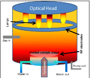
2.2.3.1. Apparatus ... 85
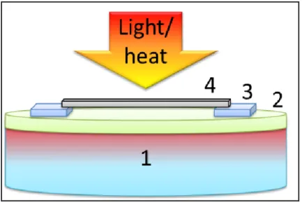
2.2.3.2. Process ... 87
2.2.4. Electrophoretic Deposition (EPD) ... 89
2.2.4.1. Electrophoretic Deposition of Graphene ... 90
2.2.5. Graphene Coated BPPs for PEMFC ... 91
2.3. Conclusions ... 94
3. Electrochemistry of Corrosion ... 97
3.1. Fundamentals of Corrosion... 97
3.1.1. Introduction to Corrosion ... 97
3.1.2. Types of Corrosion ... 98
3.1.2.1. Dry or Gaseous Corrosion ... 98
3.1.2.2. Aqueous Corrosion ... 99
3.1.2.3. Uniform Corrosion of Single Metal ... 102
3.1.2.4. Non-Uniform or Localised Corrosion ... 106
3.1.3. Summary ... 111
10
3.2.1. AC Methods: Electrochemical Impedance Spectroscopy (EIS) 112
3.2.1.1. Simple Circuit presentations98,99 ... 116
3.2.1.2. Fuel Cell Applications of EIS ... 119
3.2.2. DC Methods: Potentiodynamic Polarisation Technique ... 121
3.2.2.1. Corrosion Rate Measurements by Tafel Extrapolation 123 3.2.3. Summary ... 134
3.3. Conclusions ... 135
4. Testing Methodology ... 136
4.1. Electrochemical Test Methods ... 137
4.1.1. Interfacial Contact Resistance (ICR) Testing Methodology Using Electrochemical Impedance Spectroscopy (EIS)... 137
4.1.2. Corrosion Reaction Cell (AVESTA Cell)104 ... 140
4.1.3. Potentiodynamic Polarisation Tests ... 142
4.1.4. Potentiostatic Tests ... 142
4.1.5. Accelerated Corrosion Tests ... 143
4.1.6. In situ Fuel Cell Operation ... 143
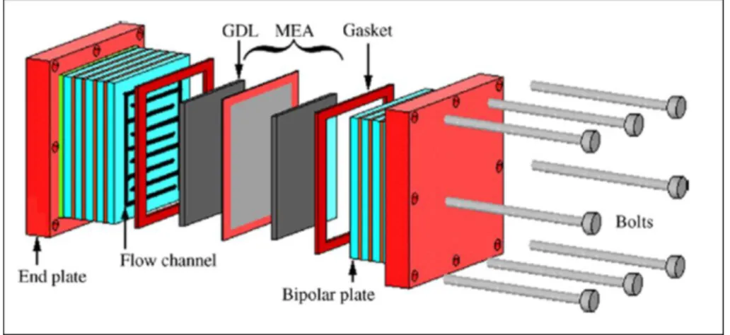
4.1.6.1. Fuel Cell Assembly ... 143
4.1.6.2. Methodology for Making MEAs ... 146
4.2. Surface Analysis ... 146
4.2.1. Scanning Electron Microscopy (SEM) ... 146
4.2.1.1. Application of SEM in Corrosion Studies ... 148
4.2.2. Atomic Force Microscopy (AFM) ... 150
4.2.2.1. Instrumentation ... 152
4.2.2.2. AFM Modes ... 153
4.2.2.3. Application of AFM ... 154
4.2.3. Raman Spectroscopy for 2D Carbon Compounds ... 156
4.2.3.1. The Raman Effect ... 156
4.2.3.2. Raman Spectroscopy of Graphene ... 159
4.2.4. 3D X-Ray Microtomography... 162
4.2.4.1. A Brief History of X-Ray Tomography ... 163
11
4.2.4.3. Lab Scale X-Ray Tomography ... 164
4.2.4.4. Application of X-Ray Tomography in Corrosion ... 165
5. Electrochemical Corrosion Analysis ... 170
5.1. ICR Test Results ... 171
5.2. Potentiodynamic Polarisation Results ... 173
5.3. Potentiostatic Tests ... 178
5.4. Accelerated Corrosion Tests ... 179
5.4.1. SEM Imaging ... 184
5.5. In situ Fuel Cell Test Results ... 189
5.6. Conclusions ... 193
6. Graphene Coatings for Steel ... 195
6.1. Photo-Thermal Chemical Vapor Deposition (PTCVD) of Graphene on Steel ... 195
6.1.1. ICR Test Results (Batch 1 with Catalyst Layer) ... 196
6.1.2. Potentiodynamic Polarisation Test Results (Batch 1 with Catalyst Layer) ... 198
6.1.3. Raman Analysis of Graphene Coating (Batch 1 with Catalyst Layer) 204 6.1.4. Post Corrosion SEM Imaging (Batch 1 with Catalyst Layer) 206 6.1.5. Batch 2 Graphene Coating without Catalyst Layer ... 209
6.1.5.1. ICR Test Results (Batch 2 without Catalyst Layer) ... 209
6.1.5.2. Potentiodynamic Polarisation Test Results (Batch 2 without Catalyst Layer) ... 211
6.1.6. Conclusions ... 215
6.2. Electrophoretic Deposition of Graphene ... 216
6.2.1. EPD Method ... 216
6.2.1.1. Graphite Intercalation Compounds ... 216
6.2.1.2. Colloidal Solution ... 218
6.2.1.3. EPD Set-up ... 218
6.2.2. EPD Results and Graphene Characterisation ... 220
12
6.2.2.2. EPD of Graphene using 50 𝑉 for 48 ℎ ... 221
6.2.2.3. EPD of Graphene using 1 𝑉 for 48 ℎ ... 223
6.2.3. ICR Results ... 227
6.2.4. Corrosion Test Results ... 229
6.2.5. Conclusions ... 230
7. 3D X-Ray Microtomography for Corrosion Analysis ... 231
7.1. Post-Corrosion X-Ray CT of Graphene Coated SS 316L ... 231
7.2. X-Ray CT of SS 316L Wires ... 234
7.2.1. Uncoated SS 316L Wire ... 236
7.2.2. Graphene Coated SS 316L Wire ... 242
7.3. Conclusions ... 247
8. Conclusions and Future Work ... 248
8.1. Conclusions ... 248
8.1.1. Electrochemical Corrosion Analysis ... 249
8.1.2. Graphene Coatings for Steel ... 250
8.1.3. 3D X-Ray Microtomography for Corrosion Analysis ... 251
8.2. Future Work ... 252
8.2.1. Metallic Coatings for Mild Steel ... 252
8.2.2. Graphene Coatings for Steel ... 252
8.2.3. 3D X-Ray Tomography of Coated Wire ... 254
Dissemination ... 255
Publications ... 255
Conference Presentations (Oral) ... 255
Conference Presentations (Poster) ... 256
Industrial Reports ... 256
13
List of Figures
Figure 1.1: 𝐶𝑂2 emissions from different sources from 1750 to 2010
(adapted from3) ... 30
Figure 1.2: General concept of a hydrogen-oxygen fuel cell (adapted from7) ... 32
Figure 1.3: Types of fuel cells and their reaction ions (adapted from4) ... 35
Figure 1.4: Schematic of a PEMFC (adapted from12) ... 38
Figure 1.5: Nernst voltage as a function of temperature ... 41
Figure 1.6: Effect of exchange current density on the activation losses (Curves calculated for various values of 𝑗𝑜 with 𝛼 = 0.5, 𝑛 = 2, 𝑎𝑛𝑑 𝑇 = 295 𝐾 (adapted from7) ... 42
Figure 1.7: Resistive (Ohmic) losses in a fuel cell 𝐴𝑆𝑅 = 0.15 Ω. 𝑐𝑚2 (adapted from4) ... 43
Figure 1.8: Concentration (mass transport) losses in a fuel cell (adapted from4) ... 44
Figure 1.9: Overall voltage losses in a fuel cell and the resulting polarisation curve (adapted from4) ... 45
Figure 1.10: Schematic of a PEM fuel cell stack connected in series (reprinted from15) ... 46
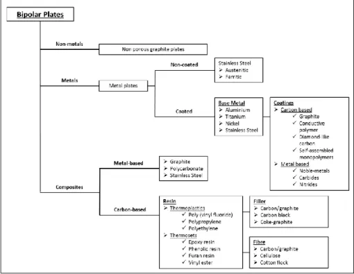
Figure 2.1: Classification of materials for BPPs used in PEM fuel cell (adapted from28) ... 54
Figure 2.2: Advantages and disadvantages of different BPP materials (adapted from16,29) ... 55
Figure 2.3: ICR values for different stainless steels and carbon paper at different compaction forces. The inset shows the ICR for different steels at a compaction force of 140 𝑁. 𝑐𝑚 − 2 (reprinted from26) ... 57
Figure 2.4: Potentiodynamic curves for SS 316L at 70 °C in 0.5𝑀 𝐻2𝑆𝑂4 bubbled with 𝐻2 or 𝑂2 (adapted from36) ... 60
Figure 2.5: A picture (left) and the schematic of the interfacial contact resistance measurement setup (adapted from41) ... 65
Figure 2.6: SEM micrograph showing a cross section of 𝑁𝑏/𝑆𝑆430/𝑁𝑏 layers (reprinted from42) ... 66
14
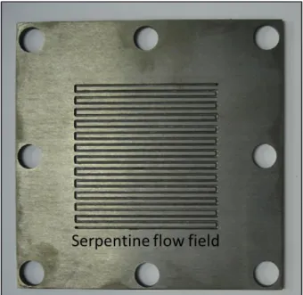
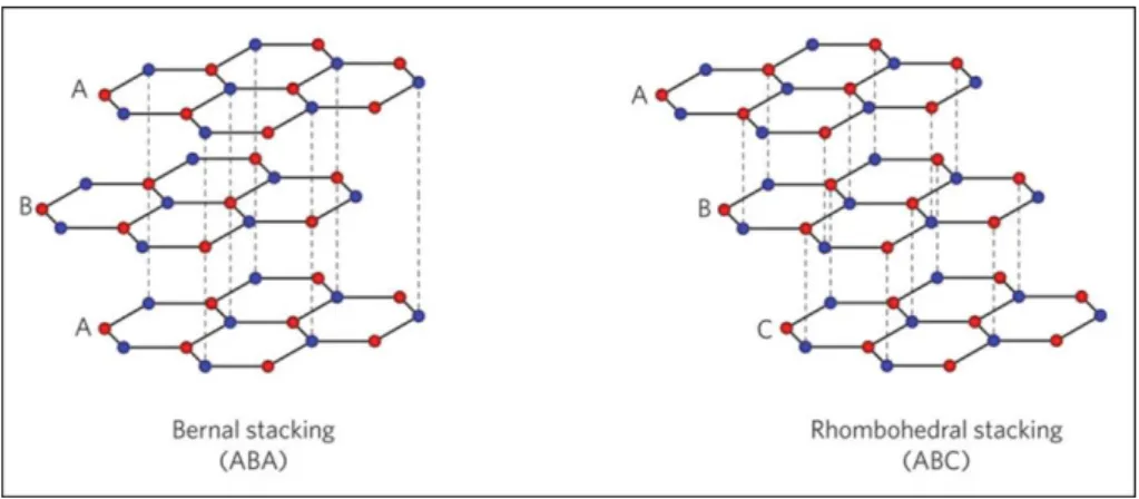
Figure 2.7: 𝑇𝑖𝑁 coated SS410: (a) 𝑇𝑖𝑁 coating surface (secondary electron image), (b) cross-sectional view of 𝑇𝑖𝑁 coating on SS 410 (secondary electron scatter), (c) cross-sectional view of 𝑇𝑖𝑁 coating on SS 410 (back-scattered electron image) (reprinted from46) ... 67 Figure 2.8: (a) Cross-sectional transition electron microscopy (TEM) image and (b) auger electron spectroscopy (AES) depth profile for L-446M stainless steel (adapted from55) ... 71 Figure 2.9: The 1045-R-𝐶𝑟(700-2) (rolling pre-treatment and chromized at 700 °C for 2 ℎ) BPP machined with a single serpentine flow field with an active surface area of 25 𝑐𝑚2 (adapted from60) ... 75 Figure 2.10: Graphite structure with individual graphene sheets stacked in AB fashion. The unit cell of graphite is shown in red lines (adapted from63) ... 78 Figure 2.11: The band structure of graphite with its Brillouin zone (adapted from63) ... 79 Figure 2.12: 𝝅 bands of graphene derived from the tight binding method (adapted from63) ... 80 Figure 2.13: AB-Bernal stacking and ABC Rhombohedral stacking in graphene (adapted from64) ... 82 Figure 2.14: Structural model of single layer graphite oxide (adapted from73) ... 84 Figure 2.15: Surrey University Nanosystems NT-1000 CVD system74 ... 86 Figure 2.16: Schematic of Surrey Nanosystems NT-1000 CVD system, showing the optical head, RF electrodes and stage cooling system74 ... 87 Figure 2.17: Positioning of the steel substrates on the cooling stage in the CVD chamber: (1) cooled sample stage, (2) silicon wafer, (3) silicon support pieces, (4) steel substrate ... 88 Figure 2.18: Schematic diagram of the two-electrode cell for electrophoretic deposition showing positively charged particles in suspension migrating towards the negative electrode (adapted from75) ... 89 Figure 2.19: Optical images of the samples and the corrosive electrolyte; SS 304 and Graphene/𝑁𝑖/SS304-900-4hr after 20 polarisation tests; (inset: an SEM image of the Graphene/𝑁𝑖/SS304-900-4hr sample with the red line outlining the metal grain boundary, the blue line outlining the graphene ripples, and the green area show the metal boundaries covered with a graphene film (adapted from85) ... 93
15
Figure 2.20: Raman spectra of the graphene-coated sample before (red curve) and after (blue curve) testing in the boiling simulated seawater (adapted from86) ... 94 Figure 3.1 :Galvanic / Daniel Cell (adapted from90) ... 101 Figure 3.2: Schematic representation of a corrosion reaction (adapted from88) ... 104 Figure 3.3: Potential-pH diagram of iron (adapted from92) ... 105 Figure 3.4: Differential aeration corrosion of steel under a droplet of water (adapted from95) ... 107 Figure 3.5: Crevice corrosion under a Type 316 bolt (adapted from94) .... 108 Figure 3.6: (a) Pitting corrosion reaction on breaching the passive layer on a stainless steel sample and (b) an example of pitting corrosion (adapted from96) ... 109 Figure 3.7: The impedance 𝑍 plotted as a planar vector using polar coordinates98 ... 116 Figure 3.8: A resistor in series with a capacitor (adapted from98,99) ... 116 Figure 3.9: A resistor in parallel with a capacitor (adapted from98,99) ... 117 Figure 3.10: A resistor in series with a constant phase element (adapted from98,99) ... 117 Figure 3.11: A resistor in parallel with a constant phase element (adapted from98,99) ... 118 Figure 3.12: A resistor in series with Warburg impedance (adapted from98,99) ... 118 Figure 3.13: A resistor in series with bounded Warburg impedance (adapted from98,99) ... 119 Figure 3.14: A resistor in series with a resistor and capacitor in parallel to each other (adapted from98,99) ... 120 Figure 3.15: A resistor in series with a resistor and constant phase element in parallel to each other (adapted from98,99) ... 120 Figure 3.16: Graph of the relationship between current and potential for a simple electrochemical reaction under activation control (adapted from90) ... 124 Figure 3.17: Electrode kinetics as expressed by the Butler–Volmer equation: (a) a symmetrical curve when 𝛼 = 0.5 and (b) an asymmetric curve when 𝛼 ≠ 0.5 (adapted from90) ... 125 Figure 3.18: Electrode kinetics as expressed by the Butler–Volmer equation, plotted in a logarithmic graph (adapted from90) ... 126
16
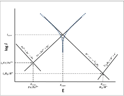
Figure 3.19: Evans diagram for actively corroding iron in an acid solution (adapted from90) ... 128 Figure 3.20: Potentiodynamic polarisation curve for SS 316L, in 1M
𝐻2𝑆𝑂4 + 2 ppm 𝐹 −ions purged with hydrogen at 80°C, at a scan rate of
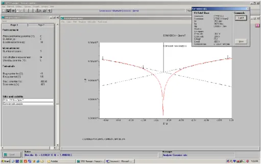
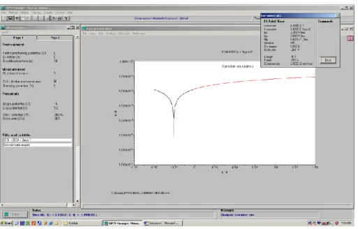
1 𝑚𝑉. 𝑠 − 1 ... 129 Figure 3.21: Portion of the Potentiodynamic polarisation curve near 𝐸𝑐𝑜𝑟𝑟 for mild steel sample, in 0.1M 𝐻2𝑆𝑂4 + 2 ppm 𝐹 −ions purged with air at 80°C, at a scan rate of 1 𝑚𝑉. 𝑠 − 1 ... 130 Figure 3.22: A screenshot of GPES software interface - Selection of Tafel region for extrapolation in order to calculate corrosion current density and hence corrosion rate ... 131 Figure 3.23: A screenshot of GPES software interface – Corrosion rate measurement by Tafel fitting after manual selection of the linear Tafel region ... 132 Figure 3.24: Demonstration of the Stern-Geary linear relationship near
𝐸𝑐𝑜𝑟𝑟 in the potentiodynamic polarisation curve for SS 316L, in 1M
𝐻2𝑆𝑂4 + 2 ppm 𝐹 −ions purged with hydrogen at 80°C, at a scan rate of
1 𝑚𝑉. 𝑠 − 1 ... 133 Figure 4.1: A schematic of the ICR testing equipment ... 138 Figure 4.2: ICR test apparatus ... 140 Figure 4.3: Schematic of the corrosion reaction cell (adapted from104) .... 141 Figure 4.4: Corrosion test apparatus ... 141 Figure 4.5: A pneumatic ram for housing a single cell fuel cell (adapted from106,107) ... 144 Figure 4.6: A schematic of the components of a single cell fuel cell (adapted from106,107) ... 145 Figure 4.7: A technical drawing for a graphite plate used as anode for fuel cell experiments(all dimensions are in 𝑚𝑚) (adapted from106,107) ... 145 Figure 4.8: SEM micrographs of A36 steel subjected to simulated (a) anode and (b) cathode conditions (bars = 50 µ𝑚) (adapted from108) ... 149 Figure 4.9: SEM micrographs of 𝑇𝑖 subjected to simulated (a and b) anode and (c and d) cathode conditions (bars = 50 µ𝑚) (adapted from108) ... 149 Figure 4.10: SEM images of SS 316L after corrosion: (a) potentiodynamic test with 𝐻2, (b) potentiodynamic test with 𝑂2, (c) potentiostatic test at
−0.1 𝑉 vs SCE with 𝐻2, and (d) potentiostatic test at 0.6 𝑉 vs SCE with 𝑂2 (bars = 10 µ𝑚) (reprinted from36) ... 150
17
Figure 4.11: Schematic of an AFM (adapted from113) ... 151 Figure 4.12: Scanning electron micrograph of an AFM tip and cantilever (bar = 20 𝜇𝑚) (adapted from112) ... 153 Figure 4.13: An AFM image of the surface of a CNT coating (adapted from114) ... 155 Figure 4.14: AFM images of carbon coated stainless steel (a) 5 µ𝑚2 and (b)
1 µ𝑚2 (adapted from115) ... 155 Figure 4.15: Schematic illustration of Raman and Rayleigh scattering and infrared absorption (adapted from116) ... 158 Figure 4.16: Lattice structure of graphene and the first brillouin zone (adapted from65) ... 160 Figure 4.17: Raman spectra of pristine and defect containing graphene (red and blue curves respectively); 𝜆 = 514.5 𝑛𝑚 (adapted from125) ... 161 Figure 4.18: (a) Comparison of the Raman spectra of graphene and graphite, measured at 514.5 𝑛𝑚. (b) Comparison of the 2D peaks in graphene and graphite (adapted from126) ... 161 Figure 4.19: (a and b) Evolution of the G peak as a function of the number of layers for 514 and 633 𝑛𝑚 excitations, and (c and d) evolution of the 2D peak as a function of the number of layers for 514 and 633 𝑛𝑚 excitations (adapted from126) ... 162 Figure 4.20: Schematic diagram of a lens-based X-ray CT system (reproduced from133) ... 164 Figure 4.21: Specimen surface of stainless steel reinforced by mortar reconstructed by X-ray tomography (reproduced from135) ... 166 Figure 4.22: Development of pitting corrosion at the bottom of the surface (reproduced from135) ... 167 Figure 4.23: (a) X-ray CT image of the surface of the sample and (b) the cross-section of the sample (reproduced from136) ... 168 Figure 4.24: X-ray CT image of steel rod (a) cross-sectional view, (b) detail of the cross-section, and (c) longitudinal 3D view (reproduced from137) .. 168 Figure 4.25: X-ray CT scans of the coupled multi-electrode array; (a) the entire array and (b) the selected electrodes (C2 and D2) (reproduced from137) ... 169 Figure 5.1: Resistance vs compression for SS 316L and functionally coated mild steel ... 172
18
Figure 5.2: Resistance vs compression for the different bare steel substrates ... 173 Figure 5.3: Potentiodynamic polarisation curves for the four bare substrates and functionally coated mild steel under air environment at 25 °C ... 174 Figure 5.4: Potentiodynamic polarisation curves for the four bare substrates and functionally coated mild steel under air environment at 80 °C ... 174 Figure 5.5: Potentiodynamic polarisation curves for the four bare substrates and functionally coated mild steel under hydrogen environment at 25 °C 175 Figure 5.6: Potentiodynamic polarisation curves for the four bare substrates and functionally coated mild steel under hydrogen environment at 80 °C 175 Figure 5.7: (a) Equivalent circuit used to fit the accelerated corrosion test data. 𝑅𝑒𝑙 is the resistance of the electrolyte, 𝑅𝑐𝑡 is the charge transfer resistance originating from the change in the surface of the working electrode and 𝐶𝑃𝐸 is the constant phase element for the working electrode. (b) gives an example of a data fit using this equivalent circuit ... 180 Figure 5.8: Electrochemical Impedance Spectra (symbols: EIS data and lines: fitted data) obtained for SS 316L under cathodic conditions (0.8 V at 23 °C in air)... 181 Figure 5.9: Change in polarisation resistance vs time for the fitted data, obtained for SS 316L under cathodic conditions (0.8 V at 23 °C in air) ... 182 Figure 5.10: Electrochemical Impedance Spectra (symbols: EIS data and lines: fitted data) obtained for SS 316L under cathodic conditions (0.8 V at 80 °C in air)... 182 Figure 5.11: Electrochemical Impedance Spectra (symbols: EIS data and lines: fitted data) obtained for SS 316L under anodic conditions (0.1 V at 23 °C in hydrogen) ... 183 Figure 5.12: Change in polarisation resistance with time for the fitted data, obtained for SS 316L under anodic conditions (0.1 V at 23 °C in hydrogen) ... 183 Figure 5.13: SEM images of SS 316L samples: (a) un-corroded, (b) air purged at 23 °C, (c) air purged at 80 °C, (d) hydrogen purged 23 °C, and (e) hydrogen purged 80 °C ... 184 Figure 5.14: SEM images of functionally coated mild steel samples: (a) non-corroded, (b) air purged at 23 °C, (c) air purged at 80 °C, and (d) hydrogen purged 23 °C ... 185 Figure 5.15: (a) SEM image of the functionally coated mild steel sample subjected to the accelerated corrosion test at 0.1 𝑉 vs RHE under a
19
hydrogen environment at 23 °C depicting pitting corrosion and coating failure, and (b) magnified image of the corrosion pit exposing the underlying mild steel ... 186 Figure 5.16: Electrochemical Impedance Spectra (symbols: EIS data and lines: fitted data) obtained for functionally coated mild steel under cathodic conditions (0.8 𝑉 at 23 °C in air) ... 187 Figure 5.17: Change in polarisation resistance with time for the fitted data, obtained for functionally coated mild steel under cathodic conditions (0.8 𝑉 at 23 °C in air) ... 187 Figure 5.18: Electrochemical Impedance Spectra (symbols: EIS data and lines: fitted data) obtained for functionally coated mild steel under cathodic conditions (0.8 𝑉 at 80 °C in air) ... 188 Figure 5.19: A schematic of SS 316L anode used to replace the graphite anode in the fuel cell ... 189 Figure 5.20: Polarisation curves for graphite/graphite and graphite/SS 316L fuel cells obtained at 80 °C ... 190 Figure 5.21: 100 ℎ fuel cell operation for graphite/graphite and graphite/SS 316L fuel cells obtained at 80°C ... 191 Figure 5.22: Optical images of (top) SS 316L and (bottom) multiple tokens of functionally coated mild steel after fuel cell operation... 192 Figure 5.23: Optical image of the contaminated MEA after use of the functionally coated mild steel BPP in in situ fuel cell operation ... 192 Figure 5.24: SEM image of the corroded holes in the functionally coated mild steel tokens ... 193 Figure 6.1: Resistance vs compression for different substrates coated with graphene with a 𝑁𝑖 catalyst layer ... 196 Figure 6.2: Potentiodynamic polarisation curves for the four substrates coated with graphene, using a 𝑁𝑖 catalyst layer, under air at 25 °C ... 199 Figure 6.3: Potentiodynamic polarisation curves for the four substrates coated with graphene, using a 𝑁𝑖 catalyst layer, under air at 80 °C ... 200 Figure 6.4: Potentiodynamic polarisation curves for the four substrates coated with graphene, using a 𝑁𝑖 catalyst layer, under hydrogen at 25 °C ... 202 Figure 6.5: Potentiodynamic polarisation curves for the four substrates coated with graphene, using a 𝑁𝑖 catalyst layer, under hydrogen at 80 °C ... 202
20
Figure 6.6: Potentiodynamic curves for SS 316L with and without a graphene coating at 80 °C under hydrogen ... 203 Figure 6.7: Raman spectra of different graphene coated samples ... 204 Figure 6.8: Raman spectra of graphene coated HILAN before and after the linear sweep corrosion scan ... 205 Figure 6.9: SEM Images of graphene coated samples, after the linear sweep corrosion scan, taken at the edge of the corroded area for (a) HILUMIN, (b) mild steel and (c) SS 316L. The left part in each image is the non-corroded graphene coating and the right part is the corroded area (bars = 200 µm) ... 207 Figure 6.10: SEM image of graphene coated SS 316L sample post corrosion scan, with coating damage and pin holes exposing bare material under the coating highlighted by the red boxes (bar = 200 µm) ... 207 Figure 6.11: A magnified SEM image of a hole in the graphene coating on the SS 316L sample (bar = 20 µm) ... 208 Figure 6.12: SEM image of the graphene coated SS 316L sample; (a) non corroded and (b) corroded areas showing corrosion under the coating as a result of the non-uniform graphene coverage (bar = 1µm) ... 208 Figure 6.13: Resistance vs compression for different substrates coated with graphene without a catalyst layer ... 210 Figure 6.14: Potentiodynamic polarisation curves for the four substrates coated with graphene without a catalyst layer under air at 25 °C ... 212 Figure 6.15: Potentiodynamic polarisation curves for the four substrates coated with graphene without a catalyst layer under air at 80 °C ... 212 Figure 6.16: Potentiodynamic polarisation curves for the four substrates coated with graphene without a catalyst layer under hydrogen at 25 °C . 213 Figure 6.17: Potentiodynamic polarisation curves for the four substrates coated with graphene without a catalyst layer under hydrogen at 80 °C . 214 Figure 6.18: Schematic diagram of the staging of graphite intercalates for stages 1 and 2, where the graphene planes are represented by connected open circles and the potassium layers are represented by the blue lines (adapted from145,146) ... 217 Figure 6.19: Schematic diagram for EPD of graphene from GIC suspension in NMP ... 220 Figure 6.20: Raman spectra of EPD graphene coated SS 316L sample using 50 𝑉 for 30 𝑚𝑖𝑛 with a 1 𝑚𝑔/𝑚𝐿 solution of GIC in NMP ... 221
21
Figure 6.21: Raman spectra of EPD graphene coated SS 316L sample using 50 𝑉 for 48 ℎ with a 3 𝑚𝑔/𝑚𝐿 solution of GIC in NMP ... 222 Figure 6.22: Optical image of EPD graphene coated SS 316L sample using
50 𝑉 for 48 ℎ with a 3 𝑚𝑔/𝑚𝐿 solution of GIC in NMP ... 222 Figure 6.23: Raman spectra of EPD graphene coated SS 316L sample using 1 𝑉 for 48 ℎ with a 3 𝑚𝑔/𝑚𝐿 solution of GIC in NMP ... 223 Figure 6.24: Optical image of EPD graphene coated SS 316L sample with a transparent graphene chunk visible on the substrate ... 224 Figure 6.25: AFM image (top) of EPD graphene coated SS 316L with the height profile (bottom) obtained on the black line ... 225 Figure 6.26: AFM image (top) of EPD graphene coated SS 316L zoomed in on the red box in Figure 6.25 with the height profile (bottom) obtained on the white line ... 226 Figure 6.27: AFM image (top) of EPD graphene coated SS 316L zoomed in on the red box in Figure 6.26 with the height profile (bottom) obtained on the white line ... 227 Figure 6.28: Resistance vs compression for uncoated and EPD graphene coated SS 316L substrate ... 228 Figure 6.29: Potentiodynamic polarisation curves for uncoated and EPD graphene coated SS 316L substrates under hydrogen at 80 °C... 229 Figure 7.1: X-ray CT image of graphene coated SS 316L token after linear sweep corrosion experiment (a) full volume rendering and (b) showing the corrosion products on the top surface ... 233 Figure 7.2: An XY-plane image (side view) of a graphene coated SS 316L token after a linear sweep corrosion experiment ... 233 Figure 7.3: An XZ-plane image (top view) of a graphene coated SS 316L token after a linear sweep corrosion experiment showing corrosion products and pits on the surface of the sample ... 234 Figure 7.4: Schematic representation of the triple phase boundary where the solid, liquid and gas phase combine to accelerate the corrosion reaction ... 235 Figure 7.5: Schematic representation of the modified bottom plate in the Avesta Cell, for attaching the wire from the bottom and eliminating the triple phase boundary ... 236 Figure 7.6:X-Ray CT image of a pristine SS 316L wire: (a) full volume rendering, (b) XZ-plane slices and (c) XY-plane ortho-slices ... 237
22
Figure 7.7: 3D volume rendering of a corroded SS 316L wire showing the texture on the surface of the wire as a result of general corrosion (left). A magnified tomograph of the corrosion pit on the surface of the wire (upper right) and the dimensions of the pit (lower right), formed as a result of pitting corrosion, are given. ... 238 Figure 7.8: 3D reconstruction of the pit by recreating surface from the data of the void. ... 239 Figure 7.9: 3D volume rendering of a corroded SS 316L wire showing the surface of the wire (left) and the XY-plane ortho-slices (right) depicting multiple pits on the wire surface. ... 240 Figure 7.10: 3D volume rendering of a corroded SS 316L wire showing the surface of the wire with multiple pits individually coloured for VSSA analysis ... 242 Figure 7.11:X-Ray CT image of an un-corroded graphene coated SS 316L wire: (a) full volume rendering, (b) XZ-plane slices and (c) XY-plane ortho-slices ... 243 Figure 7.12: Full volume rendering X-Ray CT image of graphene coated SS 316L wire corroded for 2 ℎ, showing different surfaces of the full wire... 244 Figure 7.13: Full volume rendering X-Ray CT image of graphene coated SS 316L wire corroded for 4 ℎ showing different surfaces of the full wire... 245 Figure 7.14: Full volume rendering X-Ray CT image of graphene coated SS 316L wire corroded for 12 ℎ showing different surfaces of the full wire .... 246 Figure 7.15: Comparison of the XY-plane ortho slices of graphene coated SS 316L wire corroded for (a) 2 ℎ, (b) 4 ℎ ,and (c) 12 ℎ ... 246 Figure 8.1: A schematic of DLC and graphene coating on steel to improve ICR and corrosion performance of steel ... 253 Figure 8.2: A schematic of epoxy resin covered steel wire for X-ray CT scans with the corroded exposed area ... 254
23
List of Tables
Table 1.1: A brief history of fuel cells (adapted from10,11) ... 33 Table 2.1: DOE technical targets for BPPs (adapted from21) ... 51 Table 2.2: Summary of PEM fuel cell BPP design requirements (adapted from14,16,22,23) ... 52 Table 2.3: A review of various SS samples used for BPP applications and the analysis tests conducted ... 61 Table 2.4: Chemical composition of the AISI 1045 steel (adapted from59) . 73 Table 2.5: The chemical composition of the experimental low-carbon steel AISI 102061 ... 76 Table 2.6: Typical CVD Process Parameters ... 89 Table 5.1: ICR values at 140 N cm-2 for bare substrates and functionally coated mild steel ... 171 Table 5.2: Corrosion current densities in terms of µ𝐴. 𝑐𝑚 − 2 under different conditions for the four bare substrates and functionally coated mild steel177 Table 5.3: Rate of corrosion in terms of mm per year under different conditions for the four bare substrates and functionally coated mild steel177 Table 5.4: Anodic and cathodic potentiostatic current response for SS 316L, mild steel and functionally coated mild steel ... 178 Table 5.5: Parameters used for fuel cell tests ... 190 Table 6.1: ICR values at 140 𝑁. 𝑐𝑚 − 2for the four uncoated and graphene with 𝑁𝑖 catalyst layer coated samples ... 197 Table 6.2: Rate of corrosion in terms of mm per year under air environment for the four uncoated and catalyst assisted graphene coated substrates 199 Table 6.3: Rate of corrosion in terms of mm per year under hydrogen environment for the four uncoated and catalyst assisted graphene coated substrates ... 201 Table 6.4: ICR values at 140 𝑁. 𝑐𝑚 − 2for the four substrates coated with graphene, with and without the 𝑁𝑖 catalyst layer ... 210 Table 6.5: Rate of corrosion (mm per year) under air for the four graphene coated substrates produced via catalysed and un-catalysed growth routes ... 211
24
Table 6.6: Rate of corrosion (mm per year) under hydrogen for the four graphene coated substrates via catalysed and un-catalysed growth routes ... 214 Table 6.7: Corrosion current and the rate of corrosion in terms of mm per year under hydrogen at 80 °C for uncoated and EPD graphene coated SS 316L ... 230 Table 7.1: List of parameters used for X-Ray CT experiments for a graphene coated SS 316L flat token ... 232 Table 7.2: Volume analysis of the major pit formed on the sample surface ... 239 Table 7.3: Volume analysis of the pits with a 1 % of total pit volume ... 241
25
Nomenclature
Symbols and Variables
Symbol Description
∆𝑔𝑓 Gibbs free energy (𝑘𝑗. 𝑚𝑜𝑙−1)
𝑛 Avogadro’s number (6.023 × 10²³)
𝑒 Charge of electron (1.602 × 10⁻¹⁹𝑐𝑜𝑢𝑙𝑜𝑚𝑏)
𝐹 Faraday constant (96485 𝐶)
𝐸 Energy or cell voltage (𝑉)
𝐸𝑜(𝐸 𝑟𝑒𝑣)
Nernst voltage or Standard-state reversible cell voltage (𝑉)
𝑅 Universal gas constant (8.314 𝐽. 𝑚𝑜𝑙−1. 𝐾−1)
𝑇 Absolute temperature (𝐾)
𝑎 Activity of the concerned species
𝐸𝑖𝑟𝑟𝑒𝑣 Irreversible voltage loss (𝑉)
𝜂𝑎𝑐𝑡 Activation overpotential (𝑉)
𝜂𝑜ℎ𝑚𝑖𝑐 Ohmic overpotential (𝑉)
𝜂𝑐𝑜𝑛𝑐 Concentration overpotential (𝑉)
𝛼
Charge transfer coefficient (for most reactions, 𝛼 ranges from 0.2 𝑡𝑜 0.5 and for symmetrical reactions, 𝛼 is 0.5)
𝑗 Current density (𝐴. 𝑐𝑚−2)
𝑗𝑜
Exchange current density for the reaction
(𝐴. 𝑐𝑚−2)
𝐴𝑆𝑅 Area specific resistance (Ω. 𝑐𝑚2)
𝑗𝐿 Limiting current density (𝐴. 𝑐𝑚−2)
𝐼𝐷 Raman intensity of D (disorder) peak for
graphene
𝐼𝐺 Raman intensity of G (graphitic) peak for
graphene
∅ Inner potential or Galvani potential
26
𝐽 Flux of reacting species (𝑚𝑜𝑙. 𝑐𝑚−2. 𝑠−1)
𝑉(𝑡) Instantaneous voltage (𝑉) at time 𝑡
𝑉𝑚 Maximum or peak value of voltage (𝑉)
𝜔 Angular frequency (𝑟𝑎𝑑𝑖𝑎𝑛𝑠)
𝑗(𝑡) Instantaneous current (𝐴) at time 𝑡
𝑗𝑚 Maximum or peak value of current (𝐴)
𝜃 Phase difference
𝐶 Capacitance
𝐿 Inductance
𝑍 (𝑗𝜔) or 𝑍 (𝜔) Impedance
𝑟 Rate of corrosion (usually 𝑚𝑚. 𝑦𝑒𝑎𝑟−1)
𝑀 Molecular weight of the corroding metal (𝑔. 𝑚𝑜𝑙−1)
𝜌 Density of metal (𝑔. 𝑐𝑚−3)
𝑖𝑐𝑜𝑟𝑟 Corrosion current density (𝐴. 𝑐𝑚−2)
𝑗𝑎 Anodic partial current density (𝐴. 𝑐𝑚−2)
𝑗𝑐 Cathodic partial current density (𝐴. 𝑐𝑚−2)
𝜂𝑎 Anodic overpotential
𝜂𝑐 Cathodic overpotential
𝑏𝑎= {2.303𝑅𝑇
(1 − 𝛼)𝑛𝐹} Anodic Tafel slope (𝑉𝑜𝑙𝑡 𝑝𝑒𝑟 𝑑𝑒𝑐𝑎𝑑𝑒) 𝑏𝑐= − {2.303𝑅𝑇 𝛼𝑛𝐹 } Cathodic Tafel slope (𝑉𝑜𝑙𝑡 𝑝𝑒𝑟 𝑑𝑒𝑐𝑎𝑑𝑒)
𝑅𝑝 Polarisation resistance (Ω) 𝐸𝑝 Energy of photon (𝑗𝑜𝑢𝑙𝑒𝑠) ℎ Planck’s constant (6.6256 × 10⁻³⁴𝑗𝑜𝑢𝑙𝑒. 𝑠𝑒𝑐) 𝑣𝑝 Frequency of photon (𝐻𝑧) 𝑐 Velocity of light (2.998 × 10⁻¹⁰𝑐𝑚. 𝑠𝑒𝑐−1) 𝜈̅ wavenumber (𝑐𝑚−1)
∆𝐸𝑚 Change in energy of molecule (𝑗𝑜𝑢𝑙𝑒𝑠)
𝑣𝑚 Frequency of molecule (𝐻𝑧)
𝑣𝑖 Frequency of incident photon (𝐻𝑧)
27
Abbreviations
2D Two dimensional 3D Three dimensional AC Alternating current
AES Auger Electron Spectroscopy AFC Alkaline Fuel Cell
AFM Atomic force microscope
AISI American Iron and Steel Institute
ASTM American Society for Testing and Materials BPP Bipolar plate
BSE Backscattered electron CPE Constant phase element CT Computed tomography CVD Chemical vapor deposition DC Direct current
DLC Diamond like carbon DMF Dimethylformamide DMFC Direct Methanol Fuel Cell
DOE United States Department of Energy EDM Electrical discharge mechanism EDS X-ray energy dispersive spectrometry EIS Electrochemical impedance spectroscopy EMF Electromotive Force
EPD Electrophoretic deposition
E-T Everhart-Thornley electron detector FLG Few layer graphene
GDL Gas diffusion layer
GIC Graphite intercalation compound
GO Graphene oxide
GO-EPD Graphene oxide electrophoretic deposition HOPG Highly oriented pyrolytic graphite
ICP/AAS Inductively coupled plasma / atomic absorption spectroscopy ICP/OES Inductively coupled plasma / optical emission spectrometry ICP-MS Inductively coupled plasma-mass spectrometry
28 ITO Indium tin oxide
LPR Linear polarisation resistance LSV Linear sweep voltammetry MCFC Molten Carbonate Fuel Cell MEA Membrane electrode assembly NMP 𝑁 −methyl-pyrrolidone
OCV or OCP Open Circuit Voltage or Open Circuit Potential PAFC Phosphoric Acid Fuel Cell
PEMFC Polymer Electrolyte Membrane Fuel Cell PGM Platinum group metal
PTCVD Photo-Thermal Chemical Vapor Deposition PVD Physical vapor deposition
RF Radio frequency
RHE Reversible hydrogen electrode SCE Saturated calomel electrode SE Secondary electron
SEM Scanning electron microscopy SOFC Solid Oxide Fuel Cell
SPM Scanning probe microscope SS Stainless Steel
STM Scanning tunnelling microscope TEM Transition electron microscopy VSSA Volume specific surface area XPS X-ray photoelectron spectroscopy XRD X-ray diffraction
29
1.
Introduction
A fuel cell is a type of an engine that electrochemically converts hydrogen fuel into electricity. Hydrogen presents a clean fuel option that can be produced abundantly and safely; in theory, an engine that burns pure hydrogen as a fuel produces almost no pollution. A brief history of the development of fuel cells is discussed, along with the types of fuel cells available. The Polymer Electrolyte Membrane Fuel Cell (PEMFC) is a type of fuel cell that has an ion-permeable polymer membrane as an electrolyte. Further, fuel cell electrochemistry and the working of PEMFC are discussed, as well as operating requirements for a range of applications. Finally, the aim and structure of the PhD thesis are discussed with the focus on a particular component of PEMFC; the bipolar plate.
1.1.
Overview
The impetus behind the success of the modern civilisation and the development of humanity is energy. Energy can be defined as the ability of a physical system to undertake work, may it be useful or otherwise and the efficiency of any system is then termed as the fraction of useful work out of the total work. Energy is available in a number of forms, such as kinetic energy, potential energy, heat, nuclear power, etc. The very existence of modern human society is predicated on operations such as agriculture, transportation, communication, and industrial production which are all based on the utilisation of different forms of energy. Traditionally, physical labour was the main source of energy, either from humans or animals, and then came the utilisation of fire, wind and water energies. The invention of steam engines then fuelled the industrial revolution. As the use of wood for fire could not keep up with the demand for energy, it led to the dawn of the use of fossil fuels and coal mining in the nineteenth century. The discovery of oil changed the way in which humans consumed fossil fuels for various energy requirements. For decades now, the major source of energy has been fossil fuels such as coal, natural gas or crude oil and today the majority of energy is still derived from these fossil fuels1.
30
The extensive use of these natural resources and the ignorance towards the consequences of their use, has led to a negative impact on the environment; including environmental pollution and extensive mining of natural resources. Energy demand and supply is the primary source of release of greenhouse gases2, and in particular, 𝐶𝑂2. Global fossil fuel 𝐶𝑂2 emissions have increased at a rapid rate in the last century and there is almost a tenfold increase in the last fifty years; this is evident from Figure 1.1 that was published by the United States Department of Energy in 20103.
Figure 1.1: 𝐶𝑂2emissions from different sources from 1750 to 2010 (adapted from3)
As a consequence, it is obvious that greenhouse gas emission, and the resultant effects of global warming, will directly impact on future energy production. Furthermore, most of the sources of energy that are used today are non-renewable; their extensive usage has led to the depletion in the amounts of fossil fuel that are available. The depletion of fossil fuels also poses a challenge for energy sustainability in future2. As a result of the depletion of fossil fuels and the emission of greenhouse gases from utilisation of these fuels, a need has arisen for a cleaner, greener and safer source of energy. In the last few decades, alternative and renewable sources of energy such as solar energy, wind energy, tidal energy, hydro energy, bio-fuels, geo-thermal energy, etc. have been explored or rediscovered. However, conventional energy sources, such as the petroleum-based products, have not been replaced completely because of
31
the fact that these alternative sources of energy are either not directly applicable for transportation purposes or there are hindrances in their applications including the power available from these sources, energy storage, infrastructure, costs, etc.
1.2.
Fuel Cell
Fuel cells are a promising alternative to combustion engines for application in the transportation sector4. A fuel cell can be defined as an electrochemical device that converts the chemical energy of the fuel directly into electrical energy5. In contrast to an internal combustion heat engine, which tend to have high energy loss due to the heat production and the mechanical work involved in the process, fuel cells produce electric current directly using oxygen and fuel. Fuel cells generate power with high efficiency as they are not limited by the conventional thermodynamic limitations of heat engines such as Carnot efficiency. In addition to this, as there is no thermal combustion involved, fuel cells produce power with minimum pollution and very low environmental impact. The remarkable difference, as compared to the internal combustion engine, is that electrical energy is produced instead of heat.
1.2.1.
A Brief History of Fuel Cells
The working of a fuel cell is similar to that of primary battery. However, the striking difference between the two can be explained in terms of the consumption of the fuel. In case of a battery, all the available chemical energy is stored within the battery and it can be described as an energy storage device. The battery stops producing electrical power when the reactants are consumed. However, a fuel cell is an energy conversion device that produces electrical power as long as the reactants (the fuel and the oxidant) are provided. In principle, fuel cells produce power continuously as long as the fuel is supplied6. The basic operation of a fuel cell can be depicted in Figure 1.2.
32
Figure 1.2: General concept of a hydrogen-oxygen fuel cell (adapted from7)
The discovery of the fuel cell operating principle is attributed to a Welsh lawyer-turned scientist, Sir William Robert Grove, in 18398. However, no real practical use was found for the technology for another century4,9, the first practical application of the fuel cell was in the United States space programme. The General Electric Company began developing fuel cells in the 1950s and was awarded the contract for the Gemini space mission in 1962. In the 1960s, improvements were made by incorporating Teflon in the catalyst layer directly adjacent to the electrolyte. Significant improvements were made in the technological developments in the early 1970s and onwards, including the application of a fully fluorinated Nafion® membrane as the membrane electrolyte. In 1993, Ballard Power Systems demonstrated fuel cell-powered buses. Significant research in the catalyst area was carried out by the Los Alamos National Laboratory and others9. By the end of the twentieth century, almost all car companies had demonstrated a fuel cell-powered vehicle with the efforts fuelled by the United States Department of Energy (DOE). Towards the onset of the twenty first century a new industry was born. The developments lead to the increase in the utilisation of active catalyst and at the same time reduced the amount of precious platinum metal needed. A number of fundamental technical breakthroughs have been achieved during the last two decades; however, there are still many challenges, such as cost reduction and improvement in durability whilst maintaining performance, which remain as
33
a barrier to the commercialisation of PEMFCs. Table 1.1 summarises the important breakthroughs achieved in the development of a fuel cell.
Table 1.1: A brief history of fuel cells (adapted from10,11)
1800 W.Nicholson & A.Carlisle describe the process of using electricity to “break” water
1839 Sir William Grove demonstrates fuel cell
1889
Separate teams: L.Mond & C.Langer / C.Wright & C.Thompson / L.Cailleteton & L.Colardeau performed various fuel cell experiments
1893 F.Ostwald describes the role of fuel cell components 1896 W.Jacques constructed a carbon battery
Early 1900s
E.Baur and students conducted experiments on high temperature devices
1959
Bacon demonstrates a practical 5 𝑘𝑊 fuel cell system
Harry Karl Ihrig fitted a modified 15 𝑘𝑊 Bacon cell to an Allis-Chalmers agricultural tractor
Allis-Chalmers went on to develop fuel cell powered forklift trucks, golf cart and submersible vessels in partnership with the US Air Force
1960s
Willard Thomas Grubb & Leonard Niedrach invented PEMFC technology at GE
The Grubb-Niedrach fuel cell was developed in cooperation with NASA and used in the Gemini space programme
International Fuel Cells (later UTC Power) developed a 1.5 𝑘𝑊 AFC for use in Apollo Space Missions, subsequently developed a 12 𝑘𝑊 AFC to provide on board power on all space shuttle flights
1970s
The oil crisis prompts development of alternative energy technologies
General Motors experimented with the hydrogen fuel cell powered Electrovan and although limited to demonstrations, it marked on of the earliest fuel cell electric vehicles
Shell involves in developing alcohol fuel cells
34 experimenting with FCEVs
Significant progress in the development of PAFC, including a
1 𝑀𝑊 unit developed by IFC
1980s
US Navy uses fuel cells in submarines
Ambitious conceptual designs for municipal utility power plant applications of up to 100 𝑀𝑊 output were published
1983 saw the beginning of fuel cell research by the Canadian company, Ballard
1990s
Large stationary fuel cells are developed for commercial and industrial locations with focus on PEMFC and SOFC
Early applications of PEMFC and DMFC including portable soldier-borne power, power for devices such as laptops and mobile phones
Advances in MCFC technology, particularly for large stationary applications sold by Fuel Cell Energy and MTU
Multiple fuel cell companies are listed on stock exchanges in the late 1990s
2000s
European Union, Canada, Japan, South Korea and the US are engaged in high profile fuel cell demonstration projects, particularly for stationary and transport fuel cells
Fuel cell buses are deployed in Europe, China and Australia
2007 Fuel cells begin to be sold commercially as stationary backup power units
2008 Honda launches the 100 𝑘𝑊 FCX Clarity fuel cell electric car
2009
Residential fuel cell micro-combined heat and power (micro CHP) units become commercially available in Japan
A number of portable fuel cell battery chargers sold Toshiba launches Dynario fuel cell battery charger 2011 Suzuki launches 2.5 𝑘𝑊 scooter in Europe
2013
IKEA opens the first hydrogen station for fuel cell forklift trucks in France
Toyota develops hydrogen fuel cell forklift prototype (Toyota Forklift)
2015 Sintropher project undertaken in the north west Europe for Hydrail (hydrogen rail) and trams
35 2016 Toyota launches the 114 𝑘𝑊 Mirai Present
date
Continuous research in a number of aspects of fuel cells to promote commercialisation for transportation and other niche applications
1.2.2.
Types of Fuel Cells
Fuel cells can be classified into different types on the basis of the electrolyte they use4,12 as shown in Figure 1.3.
Figure 1.3: Types of fuel cells and their reaction ions (adapted from4)
PEMFC use a very thin proton conductive membrane (e.g. perfluorosulphonated acid polymer), ideally less than 50 µ𝑚 thick as the electrolyte. A typical catalyst for PEMFC is platinum supported on carbon with a loading of about4 0.3 𝑚𝑔. 𝑐𝑚−2. The operating temperatures are in the range of 60 – 80 °C. PEMFC are a promising candidate for transportation applications, along with stationary power generation and portable power applications.
Alkaline Fuel Cell (AFC) use 85 𝑤𝑡% concentrated 𝐾𝑂𝐻 as an electrolyte for high temperature applications (250 °C) and 35 −
50 𝑤𝑡% for lower temperatures (<120 °C). 𝑁𝑖, 𝐴𝑔, metal oxides and noble metals are amongst the wide range of electrocatalysts that can be employed in AFC. However, the AFC is intolerant towards
36
carbon dioxide in either the fuel or the oxidant. These cells have been used in the Apollo space program and the Space Shuttles since the 1960s.
Phosphoric Acid Fuel Cell (PAFC) use phosphoric acid as the electrolyte. To retain the acid, usually, a SiC matrix is used and, as with PEMFC, platinum is the electrocatalysts in both the anode and cathode. Operating temperatures range between 150 and 200 °C. These are semi-commercially available in packages of 200 𝑘𝑊 for stationary electrical generation. Hundreds of units have been installed around the world.
Molten Carbonate Fuel Cell (MCFC) incorporate an electrolyte composed of a combination of alkali metal carbonates, retained in a ceramic matrix of 𝐿𝑖𝐴𝑙𝑂2. Operating temperatures lie between 600 to 700 °C, whereby the carbonates form a highly conductive molten salt. The carbonate ions provide the ion conduction. An advantage of using MCFC is that the high operating temperatures do not require a platinum group metal (PGM) catalyst. These are useful for stationary power generation.
Solid Oxide Fuel Cell (SOFC) use a solid, non-porous, metal oxide as the electrolyte which is usually a 𝑌2𝑂3 – stabilised 𝑂2 (𝑌𝑆𝑍). These fuel cells operate at a high temperature, ranging from 600 to 1000 °C, where the oxygen ions provide the ionic conductivity. Similar to MCFC, these do not require a PGM catalyst and are pre-commercially used for stationary power generation. However, smaller units are being developed for portable and auxiliary power in automobiles.
Direct Methanol (Alcohol) Fuel Cell (DMFC) is also sometimes referred to as a type of fuel cell which uses alcohol directly without reforming as a fuel. However, according to the classification using the type of electrolyte they use, DMFCs are essentially a type of polymer membrane fuel cell that uses methanol instead of hydrogen.
Due to the low operating temperatures, PEMFC have the advantage of quick start-up and, as the electrolyte is a solid membrane, offers resistance to gas crossover. PEMFCs have shown to be the most promising fuel cells to be developed for automobile applications and are used primarily for
37
transportation applications and some stationary applications. Due to their fast start-up time and favourable power-to-weight ratio, PEMFCs are particularly suitable for use in passenger vehicles, such as cars and buses.
For example, the 2008 Honda FCX Clarity and the 2016 Toyota Mirai are based on a hydrogen fuel cell. Some of the crucial properties of fuel cells that make them a beneficial source of energy are listed below4:
They promise a higher efficiency as compared to internal combustion heat engines.
They promise a low emission or even zero emission of greenhouse gases when operated on pure hydrogen.
The simplicity of operation is advantageous when it comes to commercialisation or mass production.
As there are no moving parts in the fuel cells, they offer a long life and resistance to wear and tear during long term operation.
Fuel cells operate quietly which makes them an attractive energy source for portable power supply, backup power and military applications.
Depending on the requirements, fuel cells can be made in a variety of sizes and weights, with power output ranging from microwatts to megawatts.
1.2.3.
Polymer Electrolyte Membrane Fuel Cell
(PEMFC)
PEM fuel cells operate at relatively low temperatures, around 80°C. Low-temperature operation allows them to start quickly and results in less wear on system components, resulting in better durability. However, it requires that a noble-metal catalyst (typically platinum) be used to separate the hydrogen's electrons and protons, adding to system cost. The platinum catalyst is also extremely sensitive to carbon monoxide poisoning, making it necessary to employ an additional reactor to reduce carbon monoxide in the fuel gas if the hydrogen is derived from a hydrocarbon fuel adding to the cost.
The overall basic reaction for the hydrogen/oxygen fuel cell can be written as:
38
𝟐𝑯𝟐+ 𝑶𝟐→ 𝟐𝑯𝟐𝑶 Equation 1.1
In order to understand the energy production, the two separate reactions can be explained as the anodic and the cathodic reactions. At the anode of an acidic PEMFC, hydrogen oxidises to produce protons (𝐻+) ions and electrons (𝑒−).
𝟐𝑯𝟐→ 𝟒𝑯++ 𝟒𝒆− Equation 1.2
At the cathode, oxygen reduces by reacting with the electrons to complete the other half reaction and produce oxygen anions (𝑂2−).
𝑶𝟐+ 𝟒𝒆−→ 𝟐𝑶𝟐− Equation 1.3
At the cathode, the protons and the anions combine to produce water.
𝟒𝑯++ 𝟐𝑶𝟐−→ 𝟐𝑯
𝟐𝑶 Equation 1.4
The electrons produced at the anode flow through an external circuit to the cathode and the protons flow through the electrolyte. The electrolyte must allow only the protons to pass through and not the electrons, hence they must then pass through the external circuit generating electricity. Figure 1.4 summarises these reactions and depicts the working principle of a single cell fuel cell.
39
1.3.
Fuel Cell Electrochemistry
As discussed, the overall reaction for PEMFC operation is written as:
𝑯𝟐+
𝟏
𝟐𝑶𝟐→ 𝑯𝟐𝑶 Equation 1.5
1.3.1.
Gibbs Free Energy
In the reaction in Equation 1.5, the product is one mole of 𝐻2𝑂 and the reactants are one mole of 𝐻2 and half a mole of 𝑂2. By definition13, the Gibbs free energy of formation is given by:
∆𝒈𝒇= ∆𝒈𝒇 𝒐𝒇 𝒑𝒓𝒐𝒅𝒖𝒄𝒕𝒔 − ∆𝒈𝒇 𝒐𝒇 𝒓𝒆𝒂𝒄𝒕𝒂𝒏𝒕𝒔
∆𝒈𝒇= (∆𝒈𝒇)𝑯𝟐𝑶− (∆𝒈𝒇)𝑯𝟐−𝟏
𝟐(∆𝒈𝒇)𝑶𝟐
Equation 1.6
The Gibbs free energy of formation is not constant and changes with the temperature and the phase of the reaction. The ∆𝑔𝑓 for the formation of one mole of water6 at 25 oC in liquid phase is −237.2 𝑘𝐽. 𝑚𝑜𝑙−1. Theoretically, if there are no other losses in the fuel cell, then all the Gibbs free energy can be converted into electrical energy. This can then be used to calculate the reversible voltage of a fuel cell.
In order to produce one molecule of water, two electrons are transferred to complete the reaction. Hence, for each mole of Hydrogen used,
2𝑛 electrons go through the circuit. If – 𝑒 is the charge of each electron, the charge that flow through the circuit is given by:
−𝟐𝒏𝒆 = −𝟐𝑭 𝒄𝒐𝒖𝒍𝒐𝒎𝒃𝒔 Equation 1.7
Where 𝑛 = Avogadro’s number (6.023 × 10²³), 𝑒 = charge of electron
(1.602 × 10⁻¹⁹) 𝑐𝑜𝑢𝑙𝑜𝑚𝑏, 𝐹 = Faraday constant (6.023 × 1023) ×
(1.602 × 10−19) = 96485 𝐶 .
If 𝐸 can be defined as the voltage of the fuel cell, the electrical work done can be defined as:
40
𝑬𝒍𝒆𝒄𝒕𝒓𝒊𝒄𝒂𝒍 𝒘𝒐𝒓𝒌 𝒅𝒐𝒏𝒆 = 𝒄𝒉𝒂𝒓𝒈𝒆 × 𝒗𝒐𝒍𝒕𝒂𝒈𝒆
= −𝟐𝑭𝑬 𝒋𝒐𝒖𝒍𝒆𝒔 Equation 1.8
Therefore, as explained earlier, given that there is no energy lost; this electrical work done would be equal to the Gibbs free energy released.
∆𝒈𝒇= −𝟐𝑭𝑬 Equation 1.9
Thus,
𝑬 =−∆𝒈𝒇
𝟐𝑭 Equation 1.10
Consequently, this fundamental equation gives the electromotive force (EMF), i.e. the reversible open circuit voltage (OCV) or open circuit potential (OCPof the hydrogen fuel cell. For example, for a fuel cell operating under standard conditions with ∆𝑔𝑓 = −237.2 𝑘𝑗. 𝑚𝑜𝑙−1
𝑬 = 𝟐𝟑𝟕𝟐𝟎𝟎
𝟐 × 𝟗𝟔𝟒𝟖𝟓= 𝟏. 𝟐𝟐𝟗 𝑽 Equation 1.11
1.3.2.
Effect of Concentration and Temperature on
Reversible Voltage: Nernst Equation
Taking into consideration the effect of temperature and the concentrations of the reactants, the resulting voltage (Nernst Voltage) is given by the Nernst equation:
𝑬 = 𝑬𝒐−𝑹𝑻
𝒏𝑭𝒍𝒏
𝒂𝑯𝟐𝑶
𝒂𝑯𝟐. 𝒂𝑶𝟎.𝟓𝟐 Equation 1.12
Where 𝐸 = Actual cell voltage (𝑉), 𝐸𝑜 = Standard-state reversible cell voltage (𝑉), 𝑅 = Universal gas constant (8.314 𝐽. 𝑚𝑜𝑙−1. 𝐾−1), 𝑇 = Absolute temperature (𝐾), 𝑛 = Number of electrons, and 𝑎 = Activity of the concerned species.
Taking into consideration the effects of temperature and the concentrations of the reactants, the resulting Nernst voltage under standard conditions can be calculated using the Nernst Equation 1.12 as follows:
41 𝑬 = 𝟏. 𝟐𝟐𝟗 −𝟖. 𝟑𝟏𝟒 × 𝟐𝟗𝟖 𝟐 × 𝟗𝟔𝟒𝟖𝟓 𝒍𝒏 𝟏 𝟏 × 𝟎. 𝟐𝟏𝟎.𝟓 = 𝟏. 𝟐𝟏𝟗 𝑽 Equation 1.13
Theoretically, the fuel cell is more efficient at lower temperatures as demonstrated in Figure 1.5. However, in practice, this does not hold true due to kinetic limitations.
Figure 1.5: Nernst voltage as a function of temperature
1.3.3.
Fuel Cell Irreversibility & Voltage Loss
The actual open circuit voltage of a fuel cell is lower than the derived theoretical estimate. The voltage losses that occur as the irreversible cell voltage or the overpotential can be attributed to three main causes: (i) Activation losses, (ii) Ohmic losses and (iii) Mass transport losses. The operating cell voltage can be represented as a sum of losses deducted from the theoretical reversible fuel cell voltage as defined by the Nernst equation.
𝑬 = 𝑬𝒓𝒆𝒗− 𝑬𝒊𝒓𝒓𝒆𝒗 = 𝑬𝒐− 𝜼
𝒂𝒄𝒕− 𝜼𝒐𝒉𝒎𝒊𝒄− 𝜼𝒄𝒐𝒏𝒄
42
Where 𝐸𝑖𝑟𝑟𝑒𝑣 = Irreversible voltage loss (𝑉), 𝜂𝑎𝑐𝑡= Activation overpotential
(𝑉), 𝜂𝑜ℎ𝑚𝑖𝑐= Ohmic overpotential (𝑉) and 𝜂𝑐𝑜𝑛𝑐 = Concentration overpotential (𝑉).
1.3.3.1.
Activation Losses
Activation overvoltage is the most important cause of voltage drop in low temperature fuel cell operations. These losses are caused by the reactions that occur at the electrode surfaces, a fraction of the voltage that is generated is lost in driving the chemical reaction that transfers the electrons from and to the electrodes. The effect of the exchange current density on the activation loss can be explained using Figure 1.6. The activation losses are inversely proportional to the exchange current densities.
Figure 1.6: Effect of exchange current density on the activation losses (Curves calculated for various values of 𝑗𝑜 with 𝛼 = 0.5, 𝑛 = 2, 𝑎𝑛𝑑 𝑇 =
295 𝐾 (adapted from7)
The amount of voltage drop is related to the current densities by the following equation.
𝜼𝒂𝒄𝒕= 𝑹𝑻
43
Where: 𝛼 = Charge transfer coefficient (for most reactions, 𝛼 ranges from
0.2 𝑡𝑜 0.5 and for symmetrical reactions, 𝛼 is 0.5), 𝑗 = Current density
(𝐴. 𝑐𝑚−2) and 𝑗
𝑜 = Exchange current density for the reaction.(𝐴. 𝑐𝑚−2).
1.3.3.2.
Ohmic Losses
The Ohmic losses can be seen through the full current range and are observed as a result of electrical resistance between the electrode-electrolyte and the resistance to the flow of electrons or ions in the electrolyte. The extent of the voltage loss is directly proportional to the current and is given by the equation:
𝜼𝒐𝒉𝒎𝒊𝒄= 𝒋. (𝑨𝑺𝑹𝒐𝒉𝒎𝒊𝒄) Equation 1.16 Where: 𝐴𝑆𝑅 = Area specific resistance (Ω. 𝑐𝑚2).
The effect of Ohmic loss on the overall cell potential can be seen in Figure 1.7.
Figure 1.7: Resistive (Ohmic) losses in a fuel cell (𝐴𝑆𝑅 = 0.15 Ω. 𝑐𝑚2) (adapted from4)