Relational Data Pre-Processing Techniques
for Improved Securities Fraud Detection
Andrew Fast, Lisa Friedland, Marc Maier
Brian Taylor, David Jensen
Department of Computer Science University of Massachusetts Amherst
Amherst MA 01003-9264 USA
[afast, lfriedl, maier, btaylor, jensen]
@cs.umass.edu
Henry G. Goldberg,John Komoroske
National Association of Securities Dealers 1725 K Street NW
Washington, DC 20006-1516 USA
[henry.goldberg,
john.komoroske]@nasd.com
ABSTRACT
Commercial datasets are often large, relational and dynamic. They contain many records of people, places, things and events and their interactions over time. Such datasets are rarely structured appropriately for important knowledge discovery tasks, and they often contain variables whose meaning changes across different subsets of the data. We describe how these challenges were addressed in a collaborative analysis project undertaken by the University of Massachusetts Amherst and the National Association of Securities Dealers (NASD). We describe several methods for data pre-processing that we applied to transform a large, dynamic, and relational dataset describing nearly the entirety of the U.S. securities industry, and we show how these methods made the dataset suitable for learning statistical relational models. To better utilize social structure, we first applied known consolidation and link formation techniques to associate individuals with branch office locations. In addition, we developed an innovative technique to infer professional associations by exploiting dynamic employment histories. Finally, we applied normalization techniques to create a suitable class label that adjusts for spatial, temporal, and other heterogeneity within the data. We show how these pre-processing techniques combine to provide the necessary foundation for learning high-performing statistical models of fraudulent activity.
Categories and Subject Descriptors
H.2.8 [Database Management]: Database Applications – Data Mining; I.2.6 [Artificial Intelligence]: Learning
General Terms
Algorithms, Measurement, Design, Experimentation.
Keywords
Fraud detection, data pre-processing, statistical relational learning, normalization, relational probability trees.
1.
INTRODUCTION
The National Association of Securities Dealers (NASD) is charged with overseeing and regulating over 5,000 securities firms in the United States. One primary aim of the NASD is to prevent and discover securities fraud and other forms of misconduct by member firms and their employees, called registered representatives, or reps. With over 659,000 reps currently employed, it is imperative for NASD to direct its limited regulatory resources towards the parties most likely to engage in risky behavior in the future. It is generally believed by experts at the NASD and others that fraud happens among small, interconnected groups of individuals [2]. Due to the large numbers of potential interactions between reps, timely identification of persons and groups of interest is a sizeable challenge for NASD regulators. This work is joint effort between researchers at the University of Massachusetts Amherst (UMass) and staff at the NASD to identify effective, automated methods for detecting these high-risk entities to aid NASD in their regulatory efforts.
The securities fraud domain, along with other similar domains, presents many challenges to knowledge discovery practitioners. The NASD dataset is large, containing historical records on over 3.4 million reps, 360,000 branches and over 25,000 firms. These entities also have many rich interactions over time as reps change jobs, move among branches and firms, and branches and firms change ownership. In addition, the background rate of misconduct varies over time and geography.
In this paper we describe our techniques to address each of the challenges presented by the NASD dataset. These techniques allow the transformation from raw data to high-performing models that are useful for detecting high-risk individuals. First, we utilized standard consolidation and link formation techniques as described by Goldberg and Senator [4] to infer branch entities from rep employment records. Using the inferred branch entities, we created a new technique for identifying groups of reps, which we call tribes. Tribes are groups of reps that move from branch to Permission to make digital or hard copies of all or part of this work for
personal or classroom use is granted without fee provided that copies are not made or distributed for profit or commercial advantage and that copies bear this notice and the full citation on the first page. To copy otherwise, or republish, to post on servers or to redistribute to lists, requires prior specific permission and/or a fee.
KDD’07, August 12–15, 2007, San Jose, California, USA. Copyright 2004 ACM 1-58113-000-0/00/0004…$5.00.
branch together over time. Finally, we addressed the variability in background rate by creating a normalized class label.
While the results of the data pre-processing techniques (e.g., tribes) are frequently interesting and useful in their own right, we believe their true utility lies in the integration of these various technologies to form a foundation for learning understandable and effective models for detection of securities fraud. Without this foundation of data pre-processing techniques, any analyses of large, dynamic datasets such as the NASD data run the risk of being ineffective and potentially impossible. The models we present can be used by NASD examiners to rank the risk of future misconduct by reps and branches, and these models have the added benefit of providing a means to evaluate the efficacy of our data pre-processing techniques.
In the following sections, we describe the regulatory mission of NASD and provide more details about our task and approaches. In the final section, we demonstrate the utility of our preprocessing approaches for fraud detection in complex, relational data.
2.
BACKGROUND
2.1
NASD’s Regulatory Mission
NASD is the primary private-sector regulator of the securities industry in the United States. It is currently responsible for overseeing the activities of more than 5,000 brokerage firms, 170,000 branch offices and 659,000 registered individuals. Since 1939, NASD has worked under the oversight of the U.S. Securities and Exchange Commission (SEC) to regulate all securities firms (called broker-dealers) that conduct business with the public. Currently, NASD employs a staff of over 2,500 employees situated in offices across the country and has an annual operating budget of more than $500 million.
NASD is responsible for maintaining rules that guide all phases of the business for each member, starting with the testing, registration, and licensing of prospective broker-dealers and individuals. NASD is also responsible for the surveillance, examination, and enforcement of regulatory compliance among firms. Broker-dealers that are not in compliance with NASD regulations are subject to discipline in the form of a bar or suspension from the industry, a fine, or possibly other enforcement action. In addition, NASD offers opportunities for both professional training and investor education.
In order to ensure compliance among its members, NASD utilizes two types of examinations. The first, called a cycle examination, happens on a routine basis. The second type of examination, called examination for cause, is performed in response to complaints or for other reasons. Examinations require significant time and personnel resources and are critical for ensuring the integrity of the markets and safeguarding investors. Using both types of examinations, NASD strives for the early discovery of securities violations that can prevent serious harm and lead to the timely punishment of offending parties and swift recovery of ill-gotten funds. In addition, examinations can serve to prevent future violations by emphasizing the presence of regulatory oversight.
It is imperative for NASD to identify the highest-risk branches and reps so that examiner resources can be appropriately allocated. NASD examiners currently utilize a number of different methods to identify these high-risk entities. Often these
approaches involve examining the history of regulatory or financial problems or an individual rep or branch. Due to dynamics of the marketplace and the inherent difficulty of predicting future violations, NASD is continually seeking new methods for focusing resources and identifying high-risk entities.
2.2
The Central Registration Depository
The Central Registration Depository ® (CRD) is a collection of records regarding all federally registered firms and individuals, including those registered by the SEC, NASD, the states, and other authorized regulators such as the New York Stock Exchange. This depository includes key pieces of regulatory data such as ownership and business location for firms, and employment histories for individuals. Although the information in CRD is entirely self-reported, errors, inaccuracies or missing reports can trigger regulatory action by NASD. Since 1981, when the CRD was first created, records on around 3.4 million individuals, 360,000 branches and 25,000 firms have been added to the database.
Some of the critical pieces of information for NASD’s regulatory mission are records of any disciplinary actions, typically called disclosures, filed on particular individuals. These disclosures can encompass any non-compliant actions including regulatory, criminal, or other civil judicial action. In addition, disclosures can also be in regards to customer complaints or termination agreements between firms and individual reps. Additional disclosures cover any past financial hazards an individual rep might have had such as bankruptcies, bond denials, and liens. The disclosure information found in the CRD is one of the primary sources of data on past behavior that NASD uses to assess future risk and focus their regulatory examinations to greatest effect. In addition to disclosures filed by NASD, the Broker Check System also contains disciplinary information from the SEC, state regulators, New York Stock Exchange, the FBI, and any self-reported disclosures from the firms themselves. Disclosure information for individual brokers is freely available to the public through NASD’s BrokerCheck system1.
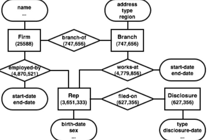
Our final analysis utilized data from the CRD for firms, branches, reps and disclosures. The compete entity-relation diagram is shown in Figure 1 along with counts for each entity appearing in our view of the database.
Figure 1: The entity-relation diagram for the CRD data.
3.
TASK DESCRIPTION
The primary goal of this work is to develop statistical models that combine patterns of past behavior, social structure among reps and firms, and the current risk environment to identify branches and reps that are at high-risk for future misconduct. To account for the dynamic nature of this process our models are designed to predict risk for the near future, given past information. This closely matches the scenario faced by NASD. Risk is broadly construed and could encompass any behavior that is potentially harmful to a member firm or to NASD as a whole.
The best available indicators of risk are the disclosure histories for reps and branches. NASD experts provided us with a weighting scheme for different disclosure types. Serious disclosures such as regulatory actions were assigned high weight while less serious disclosures such as customer complaints are given less weight. Since many disclosures with low weight may be as indicative of future misconduct as one disclosure with high weight, we combine all the disclosure types into a risk score for both reps and branches.
In a previous collaboration between UMass and NASD, it was shown that the social structure among reps was useful for detecting serious misconduct [7]. To better assess the strength of this influence among reps, this past work was limited to firms with fewer than 15 reps. In our current work, we seek to model firms of all sizes. Since the largest firms can employ hundreds if not thousands of reps, it is necessary to identify the meaningful small-scale social relations among many other incidental connections within firms. To provide the small-scale social structure we are seeking, we target two particular relations: (1) branch office affiliations and (2) tribes. Each firm typically spreads its business across many different branch locations. The branch locations must be reported to NASD; however, until recently firms were not required to report branch affiliations for their reps. To identify branch affiliations we utilized a standard consolidation and link formation technique [4] to link reps based on address reported in their employment records. More details about our approach can be found in Section 4. Due to their dynamic nature, tribes do not match standard data pre-processing techniques. We developed a novel technique to find tribes by assessing the significance of overlap in job histories between two reps. This technique is described in Section 5.
Because market conditions and corporate cultures vary widely across time and geography, it is imperative to adjust our risk measures to accurately reflect the risk environment in a particular branch or for a particular rep. For example, when the market is tight, firms may be under greater pressure to meet or surpass their goals. This pressure may manifest itself in an increased willingness to push the limits of misconduct. We show in Section 6 how normalization utilizing demographic and historical information can be used to account for variations in the risk environment.
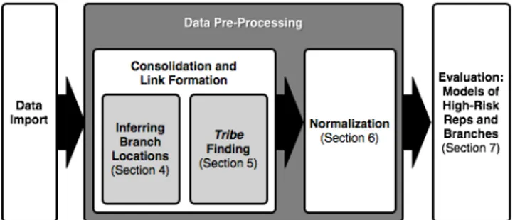
To be of use to NASD, the risk dimensions of past behavior, social structure, and risk environment must be combined into an interpretable statistical model that captures the interactions between these effects. We utilize a relational probability tree (RPT) for this purpose [6]. Along with identifying high-risk entities, we can use these models to evaluate the efficacy of our data-preprocessing techniques. The details of the RPT and results of our evaluation are described in Section 7. A graphical representation of this process is shown in Figure 2.
Figure 2: Graphical representation of the knowledge discovery process (with pointers to relevant paper sections).
4.
INFERRING BRANCH LOCATIONS
Since firms are often too large to develop an accurate view of the social relationships between brokers, we sought to link reps though employment at branch offices within each firm. There were no explicit connections between reps and branches included in the data. Each employment record for a rep, however, contained a self-reported address of employment. Unfortunately, since the addresses are self-reported, there were very few exact matches to known branch addresses.
To get a ‘fuzzy’ match between reps and branches, we used an algorithm based on Levenshtein string edit distance to determine the similarity between two addresses [10]. This algorithm assigns one point for each addition of a letter, subtraction of letter, or substitution of a letter between the two text strings. Since there can be many different ways to score points (e.g., a subtraction in the middle of a word could also be counted as a substitution), the string edit distance is the minimum possible score between two strings.
We considered addresses in two parts: (1) the street address and (2) city, state, zip. As might be expected, there are a variety of ways to express standard street address components. ‘North’ may become ‘N’, ‘N.’ or even ‘NO’. A branch that is located on ‘First Street’ may have employees that report their address as ‘1st Street’, ‘First St.,’ ‘1st St.’ etc. In order to account for these variations in street address, we started with the basic string edit distance and subtracted the difference in length for the two strings, effectively discounting the effect of abbreviations. We then divided the score by the minimum string length. The resulting score measured the percentage of characters that varied from one string to the second.
Because the city-state-zip strings have fewer common abbreviations, we chose not to subtract the difference in string length in this case. The intuition behind this is that any error in city, state, or zip code is probably a significant mismatch and should count for more. However, if the street address is identical but the city, state and zip are only slightly different then we would also like to match these addresses. To determine a final score we added the street score to the city score. If the final score was below our threshold of 0.28, then the addresses were a match. The threshold was chosen to minimize the number of false positives, i.e., branches that were truly different branches but that are grouped together by the algorithm.Examples of this approach are shown inTable 1
.
Using a threshold of 0.28, we were able to successfully match 70% (~3.35 million) of the employment records to recorded branches. The remaining 30% (~1.43 million) of employment records could not be matched to existing branches. A few
possible causes for this include branches that have moved locations over time, reps that report a home address or other non-branch address, data entry errors, or possibly multiple addresses for the same location. In many cases there were many records with the same unmatched address. Using these unique addresses (as identified by our string matching algorithm), we inferred the existence of a branch at that address. We call these branches inferred branches. We then used our matching algorithm to match the remaining 30% of the records. There were 431,895 branches recorded in the branch table. To those we added 315,761 inferred branches, for a total of 747,656 branches. Of the 315,761 inferred branches, 158,438 have a single employee.
Table 1: Example branch address matches produced by our modified string edit distance algorithm.
Successful Matches From Algorithm (True Positives) 201 E. Main St., Washington, IN, 47501
201 E. Main St. Ste. 305, Washington, IN, 47501 201 E Main Street Suite 305, Washington, IN, 47501 Incorrect Non-Matches (False Negatives) 110 Wall Street , NEW YORK, NY, 10005 110 Wall Street , NEW YORK CITY, NY, 10005 110 Wall Street , 22ND FLOOR NEW YORK, NY, 10005 110 Wall Street , NY, NY, 10005
Correct Non-Matches (True Negatives) 110 Wall Street , MANHATTAN, NY 10005 110 Wall Street , BROOKLYN, NY, 10005 110 Wall Street , BOCA RATON, FL, 33432
5.
IDENTIFYING TRIBES
In addition to the social structure provided by branch associations, we can utilize the dynamic nature of the data to identify other relations between reps. NASD experts have long suspected the existence of a pattern of behavior among reps where a group of high-risk reps, called tribes, will move together from branch office to branch office seeking ‘greener pastures’ to continue their joint activities, which may include perpetrating fraud. We developed a method to discover such tribes by identifying small groups that move together anomalously across multiple jobs. Reps can share multiple jobs by chance, due to firm and branch acquisitions and typical movement between firms and branches in the same geographic region. We wish to factor out these common trends to identify groups that stay together intentionally, sharing sequences of jobs that are unlikely to arise by chance.
To estimate the risk of the tribes we identify, we will use the risk scores on reps described in Section 6. Of course, low-risk reps can also move together in groups; a group of friends might recruit one another as they find better jobs in the industry. We expect a high-quality set of identified tribes to be homogeneous with respect to their risk scores, containing either mostly high-risk reps or mostly low-risk reps.
For our purposes, a tribe is a group of reps that have significantly similar job sequences within the industry. The tribe finding algorithm is described in more detail in a separate paper [3], but an overview follows. We enumerate all pairs of reps in the database that have ever worked together, and for each pair, we record the jobs where they have intersected. Then, our task is to decide which pairs are interesting—ideally, to distinguish which reps are choosing to be at the same jobs, versus which reps just happen to intersect in their careers. Once we determine these
significant pairs, we connect them to form tribes. The reps in a significant pair, plus any other reps connected to them through such pairs, are considered a tribe.
We use a probabilistic model to decide which pairs are interesting (i.e., significant) under a null hypothesis of reps moving independently. The key idea of the model is this: Some industry patterns are common, whether because they reflect typical career sequences, or else because whole branches may open, close, merge, or be bought. From the data, we estimate a model describing this background pattern of normal movement. For each pair of branches, it computes the percentage of reps that worked at one branch that eventually worked at the other branch as well. The employment data confirms that there are strong such trends among branches: most small branches (90%), and many large ones (30%), have some destination at which a majority of their employees later work.
To score a pair of reps, we look at the sequence of jobs they share and calculate the likelihood of that sequence according to the model. We set a cutoff, depending on how many tribes we want to produce, and all pairs with scores beyond the cutoff are rated significant.
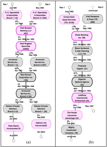
Since the real-world employment data has many instances of reps holding multiple jobs simultaneously, as well as gaps in employment records, the model was designed to handle these situations. It allows for situations where reps in a pair take any number of different jobs, then come back together. The model ignores employment durations and dates. Note that in computing probabilities, all that matters is the ordered sequence of jobs. We validated the tribes we identified using risk scores of reps and zip codes of branches. We found that the set of reps that are in tribes is strongly enriched for high risk scores: for a set of tribes containing 1600 reps, the average risk score is 8.0, compared to a global average of 0.7. Pairs of reps that are rated significant are more likely to move geographically together than other pairs that overlap by chance: they work in jobs in an average of 2.85 different zip codes, whereas the average among all candidate pairs is 1.90. Finally, the tribes are homogenous for disclosure scores. The variance within each tribe is low (i.e., each tribe is homogenous), and the variance among (average) tribe scores is high (i.e., some tribes have high scores, while some have low). We established this by permuting the assignment of the reps within tribes, estimating p< 0.001 for both measures above. Figure 3 displays the career histories of two potential tribes. Each of these tribes consists of a single pair of reps. The tribe in Figure 3(a) was scored as highly significant, while the tribe in Figure 3(b), even though it has a long history together, appears unremarkable and was scored as not significant. It is fortuitous that the brokers' start dates match, since the model does not take timing information into account. In the significant case, we interpret the synchronized movements as evidence that the brokers are coordinating their job changes. However, for the case rated insignificant, it is more likely that these transitions are sudden mass movements. As it turns out, the brokers from the significant pair have disclosure scores of 18 and 24, respectively, primarily since in April 1996 they were both fired (disclosures show an Internal Review and a Termination for each). One of the brokers from the non-significant pair has no disclosures, while the other was fired in 1997 for "diversion of profitable trades to personal" and received a score of 12 for this. In these figures, the names of the firms have been anonymized.
Figure 3: Two examples of overlapping job histories indicative of tribes. (a) An example of a significant overlap in job histories (low background probability). (b) Example of non-significant overlap (high background probability). Names of firms have been anonymized. Firm sizes are in parentheses. Edge labels display transition percentages and start dates. Bold edges indicate both reps changing employment at the same time.
Tribes can be useful for improving fraud detection in two ways. First, the tribes themselves, along with the corresponding risk scores, can direct NASD examiners towards groups of reps that merit investigation. It may also be possible to identify similarities among the tribes and identify possible tribes before branch movement is initiated. Second, due to the homogeneity of the risk scores within a tribe, we would like to incorporate these tribe relations into a combined model of risk as described in Section 7. We conducted a preliminary experiment to assess the value of using tribes to predict the risk scores of reps. First, we generated a large set of tribes, containing over 33,000 reps, by adjusting the significance threshold to be quite liberal. We converted the tribes into an attribute on reps by computing, for each rep, the average risk score of the other members of its tribe including past history up to but not including the current year. Then we constructed two training sets of reps. The first contained a mixture of reps with and without tribe attributes and the second contained only reps with defined tribe attributes. Both training sets were constructed such that half of the reps had a high risk-score and the other half had a low risk score. The scores of simple predictive rules using only the tribe attribute are shown in Table 2. They confirm that
the tribes contain predictive information. Section 7 contains more information about the modeling process.
Table 2: Using tribes to predict risk. Default Mixture Only Tribes
Accuracy 0.50 0.62 0.67
Area Under ROC 0.50 0.65 0.69
6.
NORMALIZED RISK SCORES
In order to derive a measure of risk for reps and branches, we rely heavily on disclosure information. Disclosures are a useful indicator of risk since they document and encapsulate past questionable behavior of reps. Individuals that have engaged in fraudulent activity in the past are more likely to exhibit similar behavior in the future than those with a clean history. Similarly, branches that employ reps with high risk should be deemed risky themselves. In other words, if many high-risk reps work at the same branch, then that branch might be more likely to be a source of fraudulent activity in the future.
We developed a strategy to aggregate this information into a useful statistic and used this statistic to assign an appropriate normalized class label to reps and branches. Disclosures are not distributed evenly among reps; they are highly variable. Disclosures are never filed on the vast majority of reps while some reps have many disclosures. Additionally, the frequency with which disclosures occur varies across time, geography, and types of branches. As a result, we partitioned the set of reps and branches into categories based on these three attributes and computed a risk score on reps and branches normalized by their respective category.
6.1
Normalization Categories
6.1.1
Normalization over Time
The first normalization category is temporal—by year. We limited the period under consideration to the years 1995 to 2005. This range was selected because we are mostly concerned with the immediate past, and because NASD has initiated much more comprehensive oversight and data collection. Note that 2006 is not considered since we only have partial data for that year. Figure 4 illustrates the variability of disclosures by year and justifies the need for temporal normalization. The distribution is bimodal with peaks during 1996-1997 and 2002.
Figure 4: Disclosure rates by year
6.1.2
Normalization over Geography
The second category for normalization is geographical location. We partitioned branches into ten geographical regions based on postal code. The first digit of a postal code represents a group of U.S. states that designates a population region. In the event that a branch lacks this information, we assign the branch to a geographical location by taking the majority vote from the branch’s employees’ addresses. Figure 5 depicts a map of the United States color-coded by our geographical categories. These location boundaries provide relatively equal numbers of branches within each geographical category. Note that since reps can work for multiple branches simultaneously, it is possible for a rep to appear in more than one location.
Figure 5: Zip-code regions.
6.1.3
Normalization over Branch Demographics
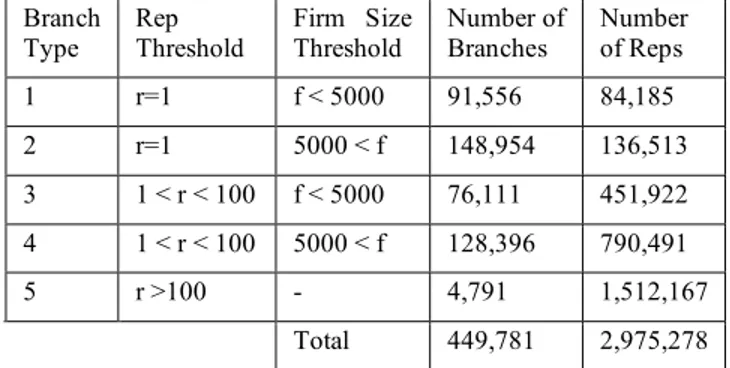
The third and final normalization category identifies types of branches. We considered two distinguishing features of branches: the size of the branch and the size of the branch’s firm (where size denotes the number of employed reps). The size of a branch/firm is the total number of unique individuals employed at the branch/firm within the period 1995-2005. We constructed partitions on these two dimensions that group branches according to size. Table 3 presents the branch typology along with the density of each class. Type 1 branches have a single rep associated with firms that employ no more than five thousand individuals. Type 2 comprises branches with a single rep for larger firms (more than five thousand reps). Types 3 and 4 contain medium-sized branches (between two and one hundred employed reps), and type 5 encompasses all remaining large branches (employing greater than one hundred reps).
Table 3: Description of Demographic Categories for Branches Branch
Type Rep Threshold Firm Size Threshold Number of Branches Number of Reps
1 r=1 f < 5000 91,556 84,185 2 r=1 5000 < f 148,954 136,513 3 1 < r < 100 f < 5000 76,111 451,922 4 1 < r < 100 5000 < f 128,396 790,491 5 r >100 - 4,791 1,512,167 Total 449,781 2,975,278
We have data on a total of 449,781 branches (both actual and inferred) that were open during our time frame, and the number of branches within each type varies. Additionally for all branch types, we have a total of 2,329,113 distinct individuals that were employed in our time frame (see Table 3). Since reps can work for multiple branches simultaneously, it is possible for the same individual to appear under multiple branch types. This accounts for the larger number appearing in Table 3. We found that roughly 28% of the employee count between 1995-2005 is attributable to multiple employments. We address the problem of attributing disclosures of reps that work several jobs simultaneously below.
6.2
Computing Risk Scores
With the normalization attributes and categories defined, we then attributed disclosures to reps and branches. First, we assigned a weight to each disclosure type based on their relative severity. Regulatory action and termination disclosures are deemed the worst type of disclosure while a judgment lien is ignored entirely. Thus, our measure of risk is a disclosure score on reps and branches. For reps, this is simply the sum of the weights of each disclosure attributed to the rep in a given year.
Next, we assigned each branch to its appropriate normalization bin based on its branch type and location. Then, for each bin, we computed the disclosure score of each branch and rep as described above. This effectively gives us distributions of rep disclosure scores and branch disclosure scores (averaged over employed reps) for each of our normalized categories of individual entities. Because an individual rep can work for multiple branches concurrently, it is important to describe how we handle multi-branch employment of reps. For reps, we assign the score in its entirety, unless multiple branches are categorized into the same bin. For branches, we designate fractional disclosure scores to each branch. This prevents so-called “bad” reps from concealing their activity by working for many branches.
Finally, we constructed a binary class label identifying entities as “high-risk” based on the normalized disclosure score. We compared the score of each entity to its expected distribution based on its normalization bin. Reps or branches were identified as being “high-risk” (positive class label) if they satisfied the following two criteria simultaneously:
1. The score was at least in the 95th percentile of all reps/branches within the category.
2. The score was above the median for all reps/branches with a non-zero score within the category.
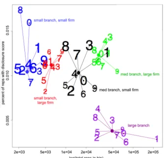
These two criteria ensure that the rep or branch is among the worst of all similar entities, but in order to limit the number, we required that they be worse than half of those entities with a non-zero score. However, if fewer than 5% of the reps in a category have scores above the median, we assign all the reps with scores above the median to the high-risk group. The remaining reps and branches were assigned a “low-risk” label (negative class label). We present data for the normalized results of reps in 2005 in . When looking at this figure, each number represents one of the normalized bins. The value of the number indicates the bin’s geographical location, the color of the number represents the branch type associated with the bin, and the size of the number is indicative of median non-zero disclosure score for the bin. The position of each number is the log of the total number of reps in the bin against the percent of reps with the disclosure score.
Figure 6: This demonstrates the need for normalized class labels by showing the variability of the disclosure scores on reps across branch demographics and regions. The larger plotted numerals indicate bins with higher median scores.
As an example, the 8 in the upper-left corner of represents the bin of small branches–small firms within the 8th geographical location. This number’s size is roughly average amongst the other numbers indicating that the median of the disclosure score for this bin is roughly average overall. This bin also has the highest percentage of reps with a disclosure score.
7.
MODELING RISK
The purpose of the evaluation described in this section is two-fold. We would like to demonstrate that we can automatically learn interpretable models of high-risk entities and we would like to demonstrate the effectiveness of our data processing approaches. We demonstrate the former by showing models automatically learned from data and demonstrate the latter by comparing our models to models learned for non-normalized class labels. This analysis was performed using PROXIMITY2, an open-source system for relational knowledge discovery designed and implemented by the Knowledge Discovery Laboratory in the Department of Computer Science at the University of Massachusetts Amherst.
7.1
The Relational Probability Tree
We utilized the relational probability tree (RPT) algorithm to learn models of high-risk reps and branches [6]. The RPT is designed to automatically construct and search over possible aggregations of heterogeneous training data. In general, instances drawn from relational data violate the independent and identically distributed (i.i.d) assumption common to most non-relational knowledge discovery techniques. The RPT applies standard aggregations COUNT, AVERAGE, MODE, etc. to effectively “propositionalize” data before selecting features to be included in the model. To find the best feature, the RPT algorithm searches over values and thresholds for each aggregator. For example, if
2 http://kdl.cs.umass.edu/proximity
we are aggregating over disclosures filed on reps then we might consider a feature such as COUNT(Disclosure.type=Bankruptcy) > 1 where the type and number of disclosure is determined by the algorithm.
The RPT is a type of probability estimation tree for relational data [8]. A probability estimation tree is similar to a classification tree, however the leaves contain a probability distribution rather than a class label assignment. Tree-based representations are often chosen for ease of interpretation and extracting meaningful rules for future use. During the training phase, the RPT algorithm learns the probability distributions for each leaf and the features for each node in the tree. These tree models can then be applied to unseen test data to determine the performance of the algorithm.
7.2
Methodology
The class label we chose for our evaluation is the normalized class label described in Section 6. As inputs, we use the attributes and structure of related entities in the network along with the intrinsic attributes on the rep or branch being evaluated. Since we are interested in predicting future behavior, our model uses information up to the present year to predict class labels that are the normalized class label in the next year. For example, our training collection consists of reps and branches that were active in 2003 and 2004. We include past information up to and including 2003 as input to our model to predict high-risk status in 2004. The testing collection follows a similar protocol but for the years 2004 and 2005. The past information includes the class label from previous years.
To generate the pool of instances from which to draw our training and test sets, we utilized the QGRAPH language implemented in PROXIMITY. QGRAPH is a graphical query language designed especially for querying large network datasets [1]. The queries used to gather instances from the database for both reps and branches are shown in Figure 7 and Figure 8, respectively. Each query returns a portion of the entire data graph called a subgraph. These subgraphs define the extent of related entities that are will considered by the RPT when creating features. For reps, we queried for only the rep themselves, their current branch affiliation, past branch affiliations (if any), and any disclosure history. For branches, we queried for the branch itself and all reps currently working at that branch and their work history (past branches and disclosures).
By definition, our normalized class label can only occur on at most 5% of the reps or branches in a given bin. To avoid any floor effects due to such a high default accuracy, we created samples that contained all of the positive instances returned by our query and undersampled the negative class so that the sample contained an equal number of positive and negative instances. Provost and Fawcett show that this procedure does not significantly affect the rankings produced by the learned model [9]. Therefore, we will evaluate our models primarily using the area under the ROC curve (AUC) metric. In order to maintain disjoint training and test sets, we removed any positive instance from the test set that also appeared in the training set. Negatives were also sampled in such a way as to avoid overlap between training and test.
Figure 7: QGraph query for reps. This query returns all reps working at a branch in the year, t, that branch, any past branches they have also worked at, and any past disclosures filed on the rep.
Figure 8: QGraph query for branches. This query returns all branches active in the given year t, all reps working at that branch during that time, any past branches those reps have worked at, and any past disclosures filed on the rep.
7.3
Empirical Evaluation
In order to assess the effect of normalization on our models, we considered two different class labels. The first class label is the normalized class label described in Section 6. We also considered a non-normalized class label that was based the top 5% of reps or branches without considering branch type and region. In addition, for each class label we considered two types of training sets for a total of four experiments each for branches and reps. We learned a single model trained on the combination of all the bins for both the normalized and non-normalized class label. We also learned a set of stratified models that were trained on each bin individually. Each of the RPTs was given attributes on reps (e.g., age, sex), branches, and disclosures (e.g., disclosure_type) as input. As described in Section 5, reps that were a part of a tribe had an additional attribute describing the average disclosure score of the other reps in the tribe. Although the tribe attributes are predictive of risk, none of these attributes were chosen in any of the models. We attribute this to the relative sparseness of tribes in the entire data. Tribes are definitely useful as a local pattern, but are not sufficiently strong to contribute to global models.
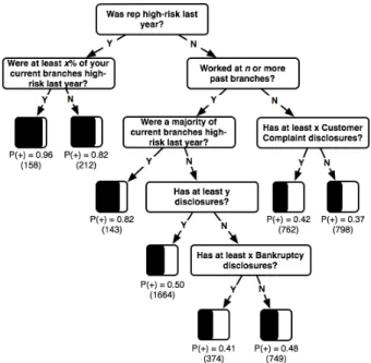
Examples of the best performing tree models for branches and reps are shown in Figure 9 and Figure 10, respectively. The features selected in these trees include the past values of the class label and attributes on related entities such as disclosures and past branches. Specific thresholds and values have been removed to avoid revealing sensitive information. The branch model was learned using the normalized class label and the rep model was learned using the non-normalized class label.
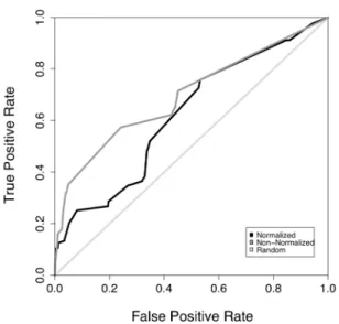
ROC curves are shown in Figure 11 and Figure 12. The performance of each of the models is summarized in Table 4. The ROC curves for normalized and non-normalized class labels were
generated by bagging the prediction of five models learned on cross-validation samples from the entire original data. The stratified models were combined from model learned on each bin individually. The stratified models perform worse than either of the models learned across the entire data. The lack of calibration between the predicted probabilities of models learned on different bins would account for the poor showing on AUC when compared to models learned on the entire data set. Unfortunately, accuracy (ACC) scores also suffer with models learned on individual bins. We attribute this effect to the reduction in sample size resulting from the stratification. Most bins have only a few positive instances, making it difficult to learn a model that generalizes well to the test sample.
Figure 9: Example branch model demonstrating the structure and types of features learned using the normalized class label.
Actual threshold values have been removed.
Figure 10: Example rep model demonstrating the structure and types of features learned using the non-normalized class
Figure 11: Normalized and non-normalized ROC curves for reps. Normalized AUC: 0.63 Non-Normalized AUC: 0.69
Table 4: Summary of Model Performance
Branch Rep
Full Stratified Full Stratified Normalized 0.76 0.57 0.63 0.55 AUC Non-normalized 0.68 0.56 0.69 0.58 Normalized 0.69 0.56 0.59 0.60 ACC Non-normalized 0.62 0.57 0.71 0.62 The highest-risk branches according to the non-normalized class labels are single person branches with a small number of disclosures. This means that some branches with relatively minor disclosure problems are ranked very highly by the non-normalized disclosure score. Other branches, perhaps with a larger number of serious disclosures but also with a larger number of reps, are pushed further down the list due the average disclosure score being low. This is the ideal situation for normalization and our normalized class label is designed to capture this concept. The branches with serious disclosures should fall near the top of their respective bin and branches with only minor disclosures should fall near the bottom of their bins. Assuming there are clear differences between the high-risk and low-risk branches, the normalized class label allows for a higher performing model. In contrast, modeling the non-normalized class label for reps produces higher performing models. Since each rep is responsible for their disclosures, there is no need to average over multiple entities. Under these conditions, the high-risk reps, regardless of bin, should have high disclosure scores and be the most probable to have future serious disclosures. The effect of normalization in this case was to exclude reps that should have been high-risk based on raw disclosure score but did not receive a positive normalized class label because they were below the 95th percentile in their bin.
Figure 12: Normalized and non-normalized ROC curves for branches. Normalized AUC: 0.76 Non-Normalized AUC: 0.68 An interesting approach to consider for normalization in the future is to have a dynamic threshold for each bin. Rather than taking the top 5% of each bin, it would be possible to take a percentage based on the overall number of disclosures appearing in that bin. For example, since disclosures are more prevalent in the smaller branches we should include a larger percentage of small branches as “high-risk” when creating normalized class labels. By varying thresholds in this way, each bin receives the same weight in the normalized class label as it carries in the original data. This may lead to improvements in modeling high-risk individuals and branches.
8.
DISCUSSION
As our results from the previous section showed, past behavior, social structure, and normalized risk assessments can be used as a foundation from which to learn high performing models from data automatically. As our learned models showed, past behavior is a strong indicator of future risk. Features aggregating past normalized disclosure scores, past disclosures, and past branch history are prominent parts of the learned models.
The creation of social structure was also useful in the modeling process. The branch entities created using consolidation and link formation techniques were foundational components in each of the aspects of our work. Despite not being chosen as a feature in our learned models, the groups of reps we identified as tribes intrigued the experts at NASD.
Based on the results of our experiments, normalization should be used with care. Normalized class labels aided in the identification of high-risk branches and should be considered as a data pre-processing technique in the future. As we saw with the rep models, creating a normalized class label did not always improve the performance of the models. There is also the potential to increase the variance of the model when sample size is small as we saw with our stratified models.
For efficiency reasons, we only considered a limited attribute set as input to the models. In the future we would like to expand the attribute set to include richer information about reps and branches that may improve fraud detection. Also, we would like to explore more ways (in addition to tribes) that are able to utilize the
temporal structure present in the data. One major consideration for future research is performing collective inference with branch and rep models to better utilize the current estimates of risk to improve over all model performance.
9.
ACKNOWLEDGMENTS
From UMass, we thank Agustin Schapira for his technical assistance, Cynthia Loiselle for her writing and editing tips, and Jennifer Neville for advice on modeling. From NASD, we thank George Walz, Dipak Thakker, Lowell Cooper, and many others for their availability, insight, and subject matter expertise. This effort is supported by the National Association of Securities Dealers through a research contract with the University of Massachusetts and the Central Intelligence Agency, the National Security Agency and National Science Foundation under NSF grant #IIS-0326249. The U.S. Government is authorized to reproduce and distribute reprints for governmental purposes notwithstanding any copyright notation hereon. The views and conclusions contained herein are those of the authors and should not be interpreted as necessarily representing the official policies or endorsements either expressed or implied, of the National Association of Securities Dealers, the Central Intelligence Agency, the National Security Agency, National Science Foundation, or the U.S. Government.
Portions of this analysis were conducted using Proximity, an open-source software environment developed by the Knowledge Discovery Laboratory at the University of Massachusetts Amherst (http://kdl.cs.umass.edu/proximity/).
10.
REFERENCES
[1] H. Blau, N. Immerman, and D. Jensen. A visual language for querying and updating graphs. Technical Report 2002-37, University of Massachusetts, 2002.
[2] C. Cortes, D. Pregibon, and C. Volinsky. Communities of interest. Lecture Notes in Computer Science, 2189:105 , 2001.
[3] Friedland, L., and Jensen, D. Finding tribes: Identifying close-knit individuals from employment patterns.
Submitted to Proceedings of the 13th ACM SIGKDD
International Conference on Knowledge Discovery and Data Mining (2007).
[4] H. G. Goldberg and T. E. Senator. Restructuring databases for knowledge discovery by consolidation and link formation. In Proceedings of the First International Conference on Knowledge Discovery and Data Mining, 1995.
[5] D. Jensen and J. Neville. Autocorrelation and linkage cause bias in evaluation of relational learners. In 12th International Conference on Inductive Logic Programming, 2002. [6] J. Neville, D. Jensen, L. Friedland, and M. Hay. Learning
relational probability trees. In Proceedings of the 9th ACM SIGKDD International Conference on Knowledge Discovery and Data Mining., 2003.
[7] J. Neville, O. Simsek, D. Jensen, J. Komoroske, K. Palmer, and H. Goldberg. Using relational knowledge discovery to prevent securities fraud. In Proceedings of the 11th ACM SIGKDD International Conference on Knowledge Discovery and Data Mining, 2005.
[8] F. Provost and P. Domingos. Tree induction of probability-based ranking. Machine Learning Journal, 52(3), 2002. [9] F. Provost and T. Fawcett. Analysis and visualization of
classifier performance comparison under imprecise class and cost distributions. In Proceedings of the 3rd International Conference on Knowledge Discovery and Data Mining, 1997.
[10]Wikipedia. Levenshtein distance — wikipedia, the free encyclopedia, 2006.