Improving Data Locality in Distributed Processing of Multi-Channel Remote Sensing Data with Potentially Large Stencils

(1)

INSTITUT F ¨

UR INFORMATIK

DER LUDWIG–MAXIMILIANS–UNIVERSIT ¨AT M ¨UNCHEN

Masterarbeit

Improving Data Locality in

Distributed Processing of

Multi-Channel Remote Sensing

Data with Potentially Large

Stencils

(2)

(3)

INSTITUT F ¨

UR INFORMATIK

DER LUDWIG–MAXIMILIANS–UNIVERSIT ¨AT M ¨UNCHEN

Masterarbeit

Improving Data Locality in

Distributed Processing of

Multi-Channel Remote Sensing

Data with Potentially Large

Stencils

Philipp Patrick Posovszky

Aufgabensteller: Prof. Dr. Dieter Kranzlm¨uller Betreuer: Pascal Jungblut

Roger Kowalewski Marc J¨ager (DLR e.V.) Abgabetermin: 06. February 2020

(4)

(5)

Hiermit versichere ich, dass ich die vorliegende Masterarbeit selbst¨andig verfasst und keine anderen als die angegebenen Quellen und Hilfsmittel verwendet habe.

M¨unchen, den 06. Februar 2020

. . . .

(6)

(7)

Abstract

Distributing a multi-channel remote sensing data processing with potentially large stencils is a difficult challenge. The goal of this master thesis was to evaluate and investigate the performance impacts of such a processing on a distributed system and if it is possible to improve the total execution time by exploiting data locality or memory alignments. The thesis also gives a brief overview of the actual state of the art in remote sensing distributed data processing and points out why distributed computing will become more important for it in the future. For the experimental part of this thesis an application to process huge arrays on a distributed system was implemented withDASH, a C++ Template Library for Distributed Data Structures with Support for Hierarchical Locality for High Performance Computing and Data-Driven Science. On the basis of the first results an optimization model was developed which has the goal to reduce network traffic while initializing a distributed data structure and executing computations on it with potentially large stencils. Furthermore, a software to estimate the memory layouts with the least network communication cost for a given multi-channel remote sensing data processing workflow was implemented. The results of this optimization were executed and evaluated afterwards. The results show that it is possible to improve the initialization speed of a large image by considering thebrick locality

by 25%. The optimization model also generate valid decisions for the initialization of the

PGAS memory layouts. However, for a real implementation the optimization model has to be modified to reflect implementation-dependent sources of overhead. This thesis presented some approaches towards solving challenges of the distributed computing world that can be used for real-world remote sensing imaging applications and contributed towards solving the challenges of the modernBig Data world for future scientific data exploitation.

(8)

(9)

1 Introduction

Remote Sensing (RS)imagery provides an important source of information about our planet e.g. allowing to monitor traffic of ships in the ocean or detect oil spilling [Vel16], to identify damage on buildings after earth quakes [YIL+13], to detect deformation and seismic activity of volcanoes [JDT+15], and to generate Digital Elevation Models (DEM) of the Earth [ZMB+_{16]. These applications emphasize the huge significance of} _RS _{imagery in business,} society and research today.

The information required for these applications is provided by spaceborne as well as air-borne systems which generate a large amount of data on a daily basis. In total more than 200 orbital senors on weather satellites, space telescopes, and observation orbiters capture remote sensing data of the Earth [MWW+_{15]. An example for such a system are the} satel-lites from theCopernicus Sentinel-2 mission from theEuropeanSpaceAgency (ESA) whose optical sensors cover the whole Earth every 5 days. The data collected between 2015 and December 2018 accumulates to a total of 6.7 petabytes (PB) which are structured in more than 13 million products [Sen18]. The sheer volume of the sensor data is a great challen in terms of storage, management, processing and analysis a challenge. TheGerman Aerospace

Center (DLR) approached these challenges in itsTanDEM-X mission by a fully automated

process that achieved to generate a DEM of the Earth out of more than 500,000 data sets [ZMB+16].

This illustrates that the processing of RS imagery can be defined as a Big Data task. Because the term Big Data is relatively new and there is no exact definition, this work will refer to it using the 4 V’s definition: Volume, Variety, Velocity, Value [HJ13]. The increasing

volume of data caused by more and more satellite missions that provide a growing variety

ofRS imagery with increasingvelocitycan be used for greatervalue applications [HSHH15]. Table 1.1 lists exemplary volumes and velocities of current satellite missions.

Because of the growth in data volume and the increasing amount of observing spaceborne and airborne missions, it seems valid to define RS as a Big Data discipline. It covers all of the 4 V’s of Big Data: (1) A large volume of data from the global missions. (2) A variety of data from different sensors. (3) An increasing value of the data for emerging businesses. (4) A high velocity of the data transfer from the sensors to the scientists. The latter is especially boosted by the change from a traditional order-request producing mode to an on-line data-triggered producing mode, which allows the scientist to have real time data access [MWW+14]. Handling the 4 V’s is a challenging task that requires modern hardware systems, high-performance data management approaches and efficient processing algorithms.

The Microwaves and Radar Institute (HR) of the DLR in Oberpfaffenhofen with its

TerraSAR-X/TanDEM-Xmission and additional airborne platforms is one of the main

play-ers in generating and processing a large amount of Synthetic Apreature Radar (SAR) RS

data. Figure 1.1 illustrates a data sets generated by a SAR sensor and the multi-temporal dimensionality. These data becomes increasingly extensive as new sensors and systems are developed. With more channels as well as a higher resolution of the imagery, the data vol-ume will likely exceed more than 1 terabyte (TB) per data set in the future. Handling such

(12)

Satellites Velocity Volumes Volumes Year (Mbps) (GB/Day) (TB/Year) HJ-1B 60.00 57 20.32 2015 HJ-1A 120.00 114 40.64 2015 [...] [...] [...] [...] [...] LANDSAT5 85.00 28.02 9.99 2015 RADARSAT-2 105.00 57.68 20.56 2015 LANDSAT8 440.00 241.70 86.16 2015 TanDEM-X* 40.00 140.00 50.00 2018 SENTINEL-2 2933.00 4124.53 1470.17 2018 Total 30143 4620 1648

Table 1.1: Satellite data center: the volume and velocity of RS data [MWW+15], [Sen18], (*Projected based on [RMW+18])

large data sets is a challenge in itself.

Figure 1.1: The dimensionality of the multi-temporalRS data.

Current techniques used to process and analyzeRS data are time consuming and expensive in terms of computational costs and related infrastructure [Vel16]. Because of optimizations of the execution time, theInput/Output (I/O)times become critical factors for the economic and scientific value of the processed data. This is particularly important for applications where a time-criticality is a requirement, such as the monitoring of the soil moisture of farmland for finding places to irrigate or oil spills to hunt the polluting ships.

Parallel programming promises a significant speedup of the processing in data-intensiveRS

(13)

1.1 Task and Definition of Goals the computational costs to distributed systems for a faster execution of the algorithms. Nev-ertheless, the required handling of multilevel hierarchies and increasingly complex distributed systems turned out to be difficult and error-prone [MWW+14]. A variety of frameworks on the market exist which proclaim to solve the issue to handle complex implementations with

MPI, such as UPC [UPC05], Titanium [YSP+98], Chapel [CCZ07] and DASH [FFK16]. These frameworks provide an abstraction layer taking care of e.g. data synchronization to simplify the algorithm development. The possible speedup of existingRS algorithms using parallel programming combined with the simplified development using a MPI abstraction framework makes the investigation of a respective solution a worthwhile project.

1.1 Task and Definition of Goals

DLR’s Microwaves and Radar Institute investigates new approaches for the processing of raw SAR data and high level products in a reliable and fast way. One of the goals is to speedup the processing time to be able to produce more and faster high level products on a big scale, like the DEM from the TanDEM-X mission [ZMB+16]. The respective RS imagery is processed requiring large stencil operations, see for a definition in Section 3.3 in Chapter 3. In the RS image processing such stencils are required to solve dependencies between several pixels in the image, e.g. to focus the image. These operations are similar to normal image processing operations like a smoothing filters, but with a way more larger extent in the stencil dimensions. Normally the stencils are in a rectangular shape. These large stencils make it difficult to parallelize the processing of the algorithm because of the data synchronization between the different nodes in the distributed system.

This work evaluates the improvement of the data locality and the data layout in a dis-tributed environment for the processing with potentially large stencils in order to reduce the communication overhead. Therefore the impact of large stencils on the communication and network saturation is analyzed and possible hardware bottlenecks in terms of network capacity and disk I/O are identified. Furthermore, a possible distribution of the data on disk aligned to theDASH patterns is investigated. At the end of the work the new approach towards optimize network traffic of the processing queue of a multi-channelRS data process-ing with prior knowledge of the stencils is evaluated. The goal is to minimize the network traffic with exploiting the locality on disk and the data layout in memory with respect to the given processing task.

1.2 Structure

The remainder of this work is structured as follows: Chapter 2 introduces the theoretical background of this work. It covers an introduction to the basics of SAR data and the processing of multi-channel data. Furthermore, a small excerpt of the current state of the art in distributed computing of RS data is summarized.

Based on this, chapter 3 defines the problem investigated in this work as well as the structure of the data used throughout this work. In addition the Portal Global Address

Space (PGAS) High Performance Computing (HPC) programming models are described

together with an introduction to theDASH framework for parallel computing.

Chapter 4 covers the optimization approach of this work. An overview over optimization strategy and the cost calculations are given. The chapter also describes the foundations of

(14)

the approach and the resulting implemented software. The software is split in one part for creating an execution plan, written in Python, and another part for processing the images, written in C++. The results of the evaluation experiments are presented and discussed in chapter 5. Afterwards, a short envision of a potential SAR HPC Processing Python API based on DASH is shown in chapter 6. The work is concluded in chapter 7.

(15)

2 Processing of Large Scale Multi-Channel

Remote Sensing Data

Multi channel data sets have become important in many fields of science. The mankind is developing better methods to measure physic abilities with increasing rapidity and so also the data sets are growing in dimensionality and size, see Figure 1.1. Especially the earth observation scientists were able to increasing the data amount in the last decades with more and cheaper satellites. Handling this amount of data is a huge challenge. In the next section an overview about the challenges in working with a large amount of RS data is given. In the follow section the physical limits of processing on new hardware developments is shown. The chapter concludes with the introduction of the distributed computing concept for RS

image processing.

2.1 Remote Sensing Images and Processing Images

In the last years various new approaches to handle RS data on distributed systems where initiated resulting in growing research in the field of RS Big Data. Many scientists are working on solutions for theRS Big Data issues that allow future researchers to successfully analyze the huge amount of availableRS data. In addition to that, large companies generate new businesses out of the emerging data and invest in research for mastering the mountain of data. With the open access policy ofESA’s Copernicus mission data, Google join the stage with its cloud platformGoogle Earth Engine which provides a platform with simple abstract access to the data and globally distributed computer centers in the background [GHD+17]. One of the first results on a global scale is an urban footprint layer generated from hundred of thousands of Landsat and Sentinel-1 scenes on the Google Earth Engine cloud platform [GM ¨U+17]. In the future these data and the developed processing techniques will be useful in various kinds of applications with great value for humankind. For example it will be possible to monitor the growth of a field with satellite images [LSBBH11], measure the soil moisture to enhance the yield of harvest [BAZ12], or monitor the environmental pollution of the ocean by ships in real time [Vel16].

The overview paper “Remote sensing big data computing: Challenges and opportuni-ties“[MWW+15] points out that the fieldRS Big Data leads to five main research issues:

• Efficient management of the large data volumes.

• Loading and distribution ofRS data.

• Irregular data access on parallel file systems.

• Complex dependencies between task and data.

(16)

In the remainder of this section the five research issues are described in more detail and some examples for solutions are given.

2.1.1 Efficient Management of the Large Data Volumes

Managing the rapidly growing amount of RS data is a difficult challenge especially as new globally distributed data centers arise resulting in the first and second issue. First, the data centers should have easily accessible systems, so that scientists can query the metadata and order/process data in a fast way. This in combination with the multi dimensionality of RS

data, see Figure 1.1, makes storing and accessing distributed RS data complex. Second, the synchronization between data centers or the transfer of the data to the scientist’s processing resources takes a lot of time. In the best case the data would be processed directly on the storing location which results in a data center which have to provide storage and computing power together. Provide storage, computing power and the common infrastructure together with the concepts to store the data efficient and manage them is expensively and can only be achieved by large players.

2.1.2 Loading and Distribution of RS Data

The computation of each pixel usually depends on a large amount of pixels in the neigh-borhood or data from another spectral band, see Section 3.6. Through this dependencies it is not easily possible to decompose the data in several data chunks and computed inde-pendently. If the data is distributed to many nodes and the low-level MPI is used, this could result in repeated calling of MPI send/receive communication which results in a sig-nificant performance decline. This is a main concern in this thesis and is deeper described in Section 3.7.

2.1.3 Irregular Data Access on Parallel File Systems

The complex dependencies between tasks and data. An example therefore is scientist uses data from a radar satellite and an optical satellite from different data centers, or just pro-cesses a time series, so the data still have to transfer and be accessible in a fast way on the localfilesystems (FS) [MWW+_{15]. This is addressed in [WMZ}+_{15], accessing multiple} files could be a performance issue for a parallel file systems, likeGeneralpurposefilesystem

(GPFS) from IBM [IBM19], which are used in modern environments and are often opti-mized for contiguous file access. [WMZ+_{15] shows one promising approach towards solving} the I/O issue is the use of a modified OrangeFS file system with application-aware data layout policies for RS image processing. A 20 to 30 percent I/O performance improvement was obtained, mainly by segmenting the RS image into multiple bricks and use a Hilbert Curve to distribute them on the I/O servers. The data inside the brick was ordered with Z-order curves.

2.1.4 Complex Dependencies between Tasks and Data

To solve specific research tasks the fusion of many different data set is necessary, e.g. in RS

to generate a image it have to be geo-referenced to the correct position of the earths surface which requires several other data sets, like the airplane flight trajectory/satellite orbit data. Also the results from a specific task could be depend on other task, which could be make

(17)

2.2 Hardware Limitations the whole processing chain quite complicated. [SBL+17] shows examples for solving the dependencies between different data and reduce the complexity with a data-cube.

2.1.5 Efficient and Productive Programming of RS Applications on Distributed Systems

The efficient and productive programming of RS applications on distributed systems de-pends on all four previous mentioned research issues. (1) Without an easy way to integrate data access in the to developed applications it is not possible to process data in a fast way. (2) Decompose the data in several chunks, process these data on a distributed system with thousand of nodes and summarize the results is much more complicated than just process everything on one single node. (3) the common file systems are not aligned to the irregular data access. (4) data fusion of distributed data on top results in a complicated data handling and fusion. Another problem is the different system architectures that exist today: from personal computers and servers to huge clustered servers and supercomputers, each with its own challenges. [PDCK11] investigates the trend in RS distributed computing to use retired personal computers with an MPI-based application to distribute the work showing that in such heterogeneous platforms additional considerations twoards load balancing are necessary. The article also compares applications for such a personal computer cluster with applications written for Graphical Processing Unit (GPU) or Field Programmable Gate

Array (FPGA) systems [PDCK11]. This different architectures of processors must also be

considered in terms of their ability to efficiently process distributed remote sensing data. In the paper “High performance GPU computing based approaches for oil spill detection from multi-temporal remote sensing data“[BDK+17] a significant speedup was demonstrated by using MPI with 64 cores for attribute computations. But still this was far away from prov-ing real scalability of these effects on huge High Performance Computing (HPC) systems. Generally speaking, a good scalability means e.g. that more speed is achieved when using more resources, for a more detailed definition see [Bon00]. At best, the amount of resources added correlates to the increase in speedup, but this is not achievable in the real world due toAmdahl’s Law, see Section 5.2.2.

All this together makes it difficult to implement efficient programming for distributed processing of distributed RS data. But this does not only apply to RS images distributed processing, most of the points are also applicable to Big data in general.

2.2 Hardware Limitations

Powerful computer systems are needed to process the large amount ofRS data. Today there are different kinds of computers, e.g. with up to 24 cores per CPU and up to 1 TB RAM [Int19], file systems up to exabyte and fast network interconnections. They are usually all structured according to the same scheme: “The von Neumann Computer Model“shown in Figure 2.1. This scheme consists of theCentral ProcessingUnits (CPU), the memory, and the devices for I/O. These components are connected using theSystem bus consisting of a

Address bus,Data bus and Control bus [von93].

CPU’s became more powerful in each technology iteration of the last decades. In the last 40 years the performance of microchips increased by the factor of 10,000 since 1978, see Figure 2.2. This development led to the postulation of the two laws: (1) The Dennard Scaling postulates the possibility to keep the current/voltage dropping and maintain the

(18)

Figure 2.1: Schema of von Neumann Computer Model

dependability between integrated circuits. (2) Moore’s Law predicts the doubling of the number of transistors per chip every year. But the performance increase per generation is falling with each new development. The flattening of the performance increase curve in the last 15 years visualizes the end of the two laws. Around 2004 the Dennard Scaling ended and more recently in 2011 theMoore’s Law has been shown to be no longer valid [HP11]. At this point more and more CPUs with parallel cores come to the market and start to bring a further performance boost, but only if the application is developed for parallel execution.

Figure 2.2: Growth in processor performance over 40 years [HP11]

The main concern is theI/Osubsystem for processingRS data, see Seciton 2.1.2 about the research issues. Modern cluster file systems likeGPFS[IBM19] allow to manage theoretically more than 633,825 yottabytes of data. So the main aspect limiting the size of the FS are the

(19)

2.3 Distributed Computing financial resources available to invest in the infrastructure. This could be quite expensive even though the cost-to-disk-space ratio has been continuously improved in the last years. But not only the size matters, but also the way to manage and access the data. As already mentioned in the previous section this could become a problem with processing RS data sets which use irregular data access patterns and are large in size itself. Even if continuous reading/writing provides good results, irregular data access can be slow and thus a potential showstopper for scaling up. Also the network interconnection is a limiting factor. First of all the delay/latency while accessing data over a network is much slower than accessing a local solid-state disk directly, because of the communication through the hardware stack from the

Processor to theI/O Subsystemover theI/O Device to another system and back again takes long then access the localI/O Device. The communication over the network with the other system could exceed the available resources, which quickly ends in a bottleneck. Adapting the network structure to cope with these problems has proven to be very costly.

As previously described it is no longer possible to rely only on hardware enhancements in the microchip architecture of general purpose systems to speed up throughput in general. One solution to gain more speedup is the development of a domain-specific architecture

that is optimized for a specific RS task. This approach promises a system that is highly efficient in processing specific RS task but does not scale to arbitrary tasks. This makes such an specific architecture expensive and maintenance intensive [HP11]. Another approach twoards an optimized processing speed is the focus on code optimization in general. This is particularly cost-intensive in terms of time, personal resources and still does not solve the problem of hardware limitations.

The DLR’s Microwaves and Radar Institute is currently using powerful servers for data intensive processing. These servers are equipped with a large amount of memory allowing to process extensive RS data sets. But to deal with the amount of data generated from the new technology digital beam forming SAR (DBFSAR) [ABA+17] system, even bigger data sets need to be handled which will start to exceed the local memory of a single node. Distributing the processing algorithms to a variety of nodes is not trivial because most of the algorithms in the institute were developed for single node processing. The scientists currently start working on parallel solutions but there is sill limited experience on this topic yet. One exception is a newly developed software that processes data via theSPARK [Apa20] framework, but an infrastructure to unleash the true potential of the SPARK framework was still not put into production.

Another solution is to use other new processing paradigms like distributed/high perfor-mance computing. In the following thesis the focus is to overcome hardware limitations with distributing the problem solution. The focus is on the improvement of data locality per processing node in the data initialization phase and improving the memory locality of the

PGAS memory space.

2.3 Distributed Computing

Distributed computing combines the resources of multiple nodes to solve a computational task. Therefore the task is divided in smaller chunks which are processed on multiple partic-ipating nodes at the same time. The workflow is managed by a server node which distributes the work chunks to client nodes which process the work packages and return the result back to the server [BCPS13]. In Figure 2.3 a simplified schema of the described work process is

(20)

shown. A master node receives a list of tasks and distributes the tasks to the available nodes for computing. After all tasks were finished the intermediate results are all communicated back to the master and then merged to a final result. The master may use a database to store the progress or intermediate results.

Figure 2.3: Simple abstract schema of a task distribution on distributed system with four nodes.

In the last decades a variety of cluster-based HPC systems appeared. One of the first projects heading towards the exploitation of clusters in RS was theNEX system of NASA, with 16 identical personal computers, with 100 MHz CPU clock speed, which are connected over Ethernet hubs to form a network [LGP+11]. This so calledBeowoulf cluster was able process its task in half of the time compared to single node processing. Today exist systems with hundred thousands of cores, like the SuperMUC-NG at the Leibniz-Rechenzentrum

in Munich which consists of 311,040 compute cores with 719 TB memory, and a peak

performance of 26.9 PetaFlops/s in the High Performance LINPACK benchmark [Rec19]. With this amount of computational power it reached the 9th place in the world ranking of

HPC systems, at the time of June 2019 [Pro19].

These cluster-basedHPC systems are often used for the processing of complex scientific data: Scientists use them to simulate the behavior of their models. Astrophysics use it to simulate the fusion of neutron stars or super novas. Chemistry and material scientists use HPC for research in quantum matter or the simulation of oxidation processes on sur-faces. Earth, climate and environmental scientists simulate the world climate or develop new weather forecast algorithms. Most of these simulations are computationally expen-sive, but some of them are also starting to become I/O intensive as well. One example is from the paper [BKBB18] the 4-D urban mapping project computed on the HPC system of the Leibniz-Rechenzentrum in Munich which already uses RS SAR products from the

TerraSAR-X satellite mission of DLR.

The general benefits of a distributed computing approach compared to a parallel appli-cation on a single node are: more resources and more possibilities to achieve scalability, better reliability, data sharing and combining heterogeneous systems. Thus benefits are at the expense of challenging system development, as mentioned in the previous section. It is technically easy to add more nodes to the system in order to increase the processing speed. But in practice, the parallel efficiency drops with the increase of CPUs, obeying theAmdahl’s law, see Section 5.2.2. One reason for this is the communication demand between the nodes while solving the computation, called the communication overhead of the algorithm. The amount of communication overhead is strongly related to the algorithm itself, problem size, number of participating cores/nodes, and data distribution. With every core that is added

(21)

2.3 Distributed Computing to the system, the amount of work per node and the part of problem it holds locally on memory is decreasing and can be solved faster. But at the same time, especially in the case of multi-channel RS image processing with a potentially large stencil, the communication overhead drastically increases, because of more dependencies to neighbor cells on a remote node. This problem is detailed in section 3.

As theRS data sets get bigger and bigger, the I/O operations will start to become a big part in the total execution time in distributed systems. To this day, most of the petascale supercomputers worldwide are not good at loading or transferring this huge amount of data. A reason for this is that locality optimization in the data storage architecture has been no main concern for such supercomputers in the past [MWW+15]. As a novel approach the

Leibniz-RechenzentruminMunichstart in 2020 aDataScienceStorage (DSS) which should solve the demands and requirements of data intensive science [Rec19].

Distributed computing is important for the processing of the growing RS data sets. A major limitation today is that current HPC systems are not designed for the high I/O

load that this type of data causes. This thesis studies an approach to account for these limitations by using the I/O of a local node and optimize the data distribution to fit to the PGAS memory layout. This should reduces the communication overhead so that the system scales better when used with multiple nodes. As a result, the use of aBeowulf cluster consisting of old personal computers or of different servers with different CPUs could become feasible for RS data processing in the HR Institute.

(22)

(23)

3 Distributed RS Image Processing

Achieving linear scale up in speed and processing is a difficult challenge. It depends on various factors, e.g. on the used algorithms, problem size, amount of processors, data layout, cache sizes and so on. The following section gives a more detailed description of our problem. It is followed by the technical background and description of the used framework.

3.1 Problem Statement

The goal is to investigate what are the effects of decompose a RS image and process them afterwards with potentially large stencils. Effects in terms of network, image reading speed from local hard drives and overall processing speed. The reason for using distributed com-puting is for a large data set with more than 1 TB, systems using aNon-Uniform Memory

Access (NUMA) architecture [BFS89] are at their limits in terms of computational

per-formance and Random Address Memory (RAM) utilization. Most of the common nodes today, such as theXeon Gold 6142 [Int19], are limited by aRAM capacity of 1 TB. Planned future releases will allow up to 4 TB. But even if the problem fits into the RAM of a single node, only a rather small number of cores can work on the data thus limiting the processing efficiency. Distributed or parallel computing could solve this issue by allowing many individual nodes to participate in the processing by sharing their resources. But with this kind of processing other problems arise. We have three key issues while transferring or writing a program for distributed or parallel computing: (1) Existing programs using a variety of computation types,structures to solve problems and this is not easy to transfer to an uniform approach. (2) The variability of the computational resources has to be addressed because the nodes could have a dissimilar amount of load or different computational capa-bilities. (3) The communication overhead has to be taken into account because inter-node communication over network is slower than inter-machine communication via the internal bus [Bok87].

For this thesis the focus is set on the third issue while using distributed computing. The first issue is mainly a problem for migrating existing applications to distributed computing. The dissimilarity in load and computational capabilities will only be a problem if there are competitive calculations in parallel or if one node is much slower. The communication overhead occurs when the processing on the nodes is not independent and intermediate results have to be exchanged to other participating nodes. This could be of particular interest forRS data operations with a huge dependency to neighborhoods using potentially large stencils on large arrays, as described in detail in the next section.

One way to minimize the communication over the network in the initializing step could be to increase the locality of data in the local storage such its aligned to thePGAS memory layout such that the demand of following processing steps with different stencils is satisfied at its best. This means in the best case, each node holds the data which are supposed to be in its part of the PGAS memory layout while the processing directly on it’s local disk, rather than loading it over network.

(24)

3.2 Data Description

The SAR data sets are structured similar to an ordinary optical image. The whole image consists of a two dimensional pixel array. Each pixel is defined by its positionx, yand a value

n for a specific physical property, e.g. the color in the case of an optical image. However, in a SAR image n specifies a complex number that represents the amplitude and phase of the electromagnetic wave. In an optical image n often consists out of multiple values that specify the position of the appropriate color in a color space, e.g. the RGB color space is defined by three channels for the light intensity of red, green and blue. A DBFSAR image also can have up to 60 channels per image and more [ABA+17]. If we assume a image with 100,000·25,000 pixels and one pixel being represented by a 8 Byte complex number, which is common for aSAR image, with 60 different channels, the resulting size is 18.62 GB. Each of these channels could be processed separately and combined for different kinds of high level products. RS images normally contains a stack of metadata, e.g for a airboren system the

flight trajectory. For this thesis the metadata are not considered.

For loading the data on different nodes in parallel they have to be segmented into bricks, like in the Figures 3.1 and 3.5 shown. There the whole image is segmented in regular quadratic blocks, called a data brick. Its also possible to segment the bricks line or column wise, to match with the later described DASH patterns. The position of the brick could be encoded with the x, y coordinate of the upper left and lower right coordinate. Each data brick will be distributed to a local FS of a participating node. A boost in I/O while reading/writing on the local disk of a single node in comparison to a parallel file system is expected. The reason is, at a certain point either the parallel file system, in particular the server, will not be able to handle moreI/O request or the speed of the network interconnect becomes a bottleneck.

In chapter 5 evaluation experiments will be performed. Instead of generating the workload with realSAR data and algorithms, artificially generated grayscale images for the input and for the processing step a smoothing algorithm for simulating the workload of potential large stencil algorithms is used, see section 4.5.2. Real DBFSAR algorithms are not used in this thesis, because of they are not available in a compatible programming language for distributed computing, like C++, right now. Another requirement is the image width and height have to be divisible by powers of two.

Despite the approach with distributed solutions it would also possible for a large image to segment it in a lot of independent smaller images and stitch them back together after the processing. However, this generates a lot of more computational overhead and complexity for the whole processing.

3.3 Stencil Computation

Following [SSPP11], stencil operations are defined as: The neighborhood is commonly de-fined by a rectangle. A simple example for such a stencil operation is to add up all cells in the neighborhood and divide them by the total count to get the mean value of the neighbor-hood. A similar calculation is used by smoothing filters in image processing. In RS image processing, and the radar signal processing in particular, the neighborhood of an update cell often becomes extremely large which leads to a problem with communication overhead over multiple nodes, as stated earlier. Also, keeping all necessary cells in the cache of the CPU

(25)

3.3 Stencil Computation

Figure 3.1: ASAR image segmented in 20 data bricks with a size of 2048·2048 pixels each.

for a single cell update will become difficult. Furthermore, as these kind of operations are of low arithmetic intensity, they hardly benefit from repeated access pattern on already loaded cache lines. This could, depending on the domain and stencil extents, generate a lot of cache misses which limits the total throughput to the node [SSPP11]. The performance of the real execution time of a stencils can become relevant for compare the different possible PGAS

layouts and estimate costs for them.

Figure 3.2 shows an exemplary stencil operation for a 5·5 array. On the center pixel a stencil is applied, which smooths the array by calculating the mean of the 3·3 neighborhood as described earlier. The resulting mean value for the center pixel in the example is 15. The requirement in this thesis for the stencil extents is to be odd, otherwise it’s not possible to have a center pixel. This is not true for radar signal processing, there are also even-sized stencils common.

(26)

3.4 DASH - a PGAS Framework

The following introduction to the DASH framework is mainly based on “DASH: A C++

PGAS Library for Distributed Data Structures and Parallel Algorithms“ [FFK16].

A partitioned global address space approach allows each participating nodes to have a global view on the data structure, e.g. an 2D array, inside and globally shared memory. Each node participate with a part of it’s local memory to the globally shared memory. This (PGAS) memory space is distributed to all nodes and can be adapted by certain patterns in the layout. Thus, the application can benefit from a large shared memory, but additionally with the possibility to control the memory layout (global or on local level) to the demands of high performance and scalability [YBC+_{07]. The possibility to control the memory layout is} a key factor for this thesis. In the following, a rough overview overPGAS approaches on the market and more details about theDASH concept are given. Next toDASH there are several otherPGAS approaches on the market, likeUPC [UPC05],Titanium [YSP+_{98], and}_Chapel [CCZ07]. But they all come as a new language, and thus with a compiler, which means a complete new ecosystem. Usually, this requires to train developers for the new language, which leads to high costs and only a few organizations can afford this. Also, it is unsure if the compiler developers continue their work and can give support in the future [FFK16]. With release ofC++11 [ISO12] and its introduced powerful abstraction mechanism for a generic, expressive and highly optimized library, many projects started to use C++11, like UPC++

[ZKD+14], Kokkos [ETS14], RAJA [HK14], and also DASH [FFK16]. Like mentioned in

Section 2.2 and Section 2.3, remote accessing and sharing memory becomes more important in distributed systems. For current and future large-scale systemsPGAS is widely considered as a promising approach. The DASH framework uses a one-sided communication model, which is based onMPI-3 Remote Memory Access (RMA) features and is the basis for the runtime system of DASH, called theDASH RunTime (DART).DASH itself is implemented as aC++ template library. In this way there is no requirement for a custom (pre-)compiler infrastructure, this is called a compiler-freePGAS [SKF18].

This thesis follows [FF16] in the use of terminology when referring toDASH features:

• unit: single CPU core which contributes storage and processing resources.

• teams: several units can be organized in hierarchical teams.

• patterns: partition the global memory of an array into blocks and map them to a

specific unit.

We have decided to use theDASH framework for testing theHPC ability of our experiment and to prove our hypothesis about improving locality on the disk while initializing a PGAS

data array and optimized the memory layout for processing of multi-channel remote sensing data with potentially large stencils.

3.5 Patterns in DASH

The features of the DASH library can be used in order to improve the data locality and avoid communication overhead. The DASH library allows to use different variants of data distribution patterns for the shared PGAS memory which can be configured by specific parameters, e.g. parameters are the array size in the dimensions, the amount of used units,

(27)

3.5 Patterns in DASH see Listing 3.1. This patterns define how the global PGAS view is build up of the memory of all units. For each dimension it is possible to choose from CYCLIC, BLOCK-CYCLIC,

TILEDandBLOCKEDpattern. If there is more than one dimension and a pattern is already

chosen, it is also possible to specifyNONE for the remaining dimensions. Listing 3.1 shows the instantiation of a NONE BLOCKED pattern. The amount of units is chosen by the

mpirun call and inside the implementations the maximum amount of units is used. It is

possible to group up the units in different teams and create a distributed array only for this team, but this feature is not used in this thesis. Per default the units are assigned to the given nodes using a round robin manner, though direct unit mapping is also possible. The version ofDASH used in this thesis does not support overlapping memory areas at the edges, so that edge areas are automatically synchronized. In the next release of DASH this feature will be usable.

Listing 3.1: Instantiation of NONE BLOCKED DASH pattern d a s h :: T e a m S p e c <2 > ts (1 , d a s h :: s i z e ( ) ) ;

d a s h :: D i s t r i b u t i o n S p e c <2 > ds ( d a s h :: NONE , d a s h :: B L O C K E D ); d a s h :: S i z e S p e c <2 > ss ( e x t e n t _ x , e x t e n t _ y );

d a s h :: Pattern <2 > p a t t e r n ( ss , ds , ts );

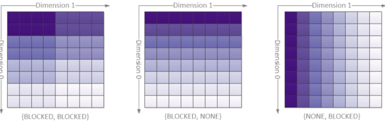
So it is possible for the application developer to specify a data distribution which achieves a high data locality in the initialization phase and communication avoidance in the processing phase, depending on the chosen pattern and stencils. Examples for the different layouts is shown in the Figure 3.3. Each color shade represents an unit, the units can be placed on independent nodes. In the following thesis we use the abbreviation B for BLOCKED and

N forNONE. As a synonme for pattern also layout can be used. Distribution could be used in both context, the brick on the disk or die blocks in the memory.

Figure 3.3: DifferentDASH patterns with 8units on a segmented image in 8·8 bricks. Each color shade represents a block on an different unit.

(28)

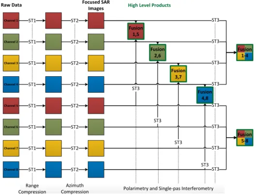
3.6 Multi-channel RS Processing Workflow

The processing of SAR or multi-channel RS images is comparable to classical image pro-cessing, just with more channels and bigger stencils. In Figure 3.4 an exemplary workflow for multi-channelRS processing with eight different channels is illustrated. Transformations that only apply to a single channel are depicted on the left side of the figure. A high level product processing step combining different channels is shown on the right side of the figure. At the end of this exemplary workflow, six high level products are generated. An example for such a product is depicted in the background of Figure 3.1.

ST2 ST1 ST2 ST2 ST3 ST3 ST3 ST3 Fusion 5-8 ST2 ST2 ST2 ST2 ST3 ST3 ST3 ST3 Fusion 1,5 ST3 Fusion 2,6 ST3 Fusion 3,7 ST3 Fusion 4,8 ST3 Channel 1 Channel 2 Channel 3 Channel 4 Channel 5 Channel 6 Channel 7 Channel 8 ST1 ST1 ST2 ST1 ST1 ST1 ST1 ST1

High Level Products

Focused SAR Images Raw Data Range Compression Azimuth

Compression Polarimetry and Single-pas Interferometry

Fusion 1-4

Figure 3.4: Multi-channelRS processing workflow

The arrows in the Figure 3.4 represent computations on the image. These computations are distinguished in computations on a single channel, calledTransformation (T), and com-binations of various channels, called Fusion (F). The transformation step preprocesses the channel in order to e.g. obtain equally illuminated scenes or focus the image in each dimen-sion. Latter is needed to account for antenna movements along the flight track of airborne

SAR systems. Fusion tasks combine different channels to generate high level products, like interferometric or polarimetric products. After each computation step the nodes have to write the intermediate results back to disk to keep them for follow-up processing. Trans-formations often use stencils with a big size in one of the dimensions (see ST1/ST2 in Figure 3.5), e.g. to compensate the proper motion the airplane in the process of focusing the

(29)

3.6 Multi-channel RS Processing Workflow stencils of Fusion operations are more square like, as depicted byST3 in Figure 3.5. General the size of the fusion stencils is by a factor of 10 smaller compared to the other stencils which could have extents up to more than 1000 pixels in width or height. In contrast to the small stencils in classical image processing with e.g. sharpener filters with stencil sizes of 3·3 or 5·5, the stencils in RS image processing could become significantly larger.

Figure 3.5: Different stencil operations: (ST1) with high extent in dimension 1, (ST2) stencil with high extent in dimension 0 and (ST3) stencil with small and similar extent in both dimensions. Color shade represent a unit.

(30)

3.7 Brick and Data Locality

The localities are distinguished between initializing the data from the hard disk into PGAS

memory, calledbrick in this context, and during processing in RAM, calledblock in this con-text. Abrick represents the data on the local disk as ann·mpixel array. Ablock represents an area in RAM of a unit. From this we distinguished between to locality concepts,brick locality andblock locality.

Brick locality is defined as the amount ofbricks which are stored on the node which will holds theblock in its local memory after the initialization.

Block locality is defined as the amount of pixel which have not to be moved to another node while switching between to layouts.

In both locality definitions there is no network transfer necessary for initializing the data or switching the memory layout. In the Figure 3.6 an simplified example for brick locality

is shown. A image is decomposed in 8·8 bricks and distributed to eight nodes and each node stores tow rows of bricks. Also it is assumed each node handle the execution of one

units, so each node is responsible for loading eight bricks. If the bricks are now initialized into an DASH array with the BB pattern, a 50% brick locality is achieved. Using a BN

pattern matches the storage pattern, which is row wise on the nodes, thus increasing the brick locality to 100%. The other way around with a NB layout, results in only 12.5%

brick locality. The bricks which are local stored on the node disk are highlighted red in the Figure 3.6. With a higher brick locality factor less bricks have to be copied to another

unit, which result in less network load. If the memory DASH pattern exactly matches the storage brick pattern, then there will be no remote calls at all and the system can read all memory from the fast local disks. With no remote calls the totalI/O speed will be no longer depending on the total throughput of the network and storage infrastructure. Instead the accumulated disk speed of all nodes is the maximum I/O which can be achieved. If brick locality is decreasing, the network will be again also an factor to consider.

Figure 3.6: Visualization of an image segmented in 8·8 bricks loaded into aBB,BN andNB

patterns inDASH using eightunits. The different block colors shades correspond to the differentunits and the brick number corresponds to the respective node. Red highlighted brick numbers are locally available on the disk.

Multi-state processing pipelines may benefit from a switch in theDASH layout between individual processing stages. The amount of traffic generated by switch the layout and processing on a aligned stencils could be less then the traffic is processing with an unaligned

(31)

3.7 Brick and Data Locality stencil.In the Figure 3.7 an simplified example for block locality is shown. Given a DASH

array with aBB pattern consist out of 8·8 bricks. If a layout switch is assumed to a BN

pattern 50% block locality is achieved. The other way around, for the NB pattern 12.5% is achieved. In contrast to in thebrick locality example, some units have no data in it’s local memory at all. While switch a layout the network decreases with a higher block locality, because less data have to be communicated to otherunits.

Figure 3.7: Visualization of an image segmented in 8·8 and already loaded into aDASH array with BB pattern. The different block colors shades and numbers correspondent to the different units/nodes. Red highlighted brick numbers are available in the local memory.

(32)

(33)

4 Optimization Model for Data Locality

The aim is to minimize the total volume of inter-node communication. For this purpose it is necessary to consider the amount of communication that is required to initialize the bricks into the memory as well as the amount of communication due to stencils processing. This can be achieved by aligning the brick distribution on the nodes to theDASH memory layout in the initialization step and additionally align the memory layout to the used stencils.

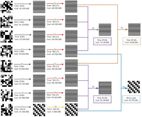
A processing chain is divided into multiple steps as described in Section 3.6 (Fig.3.4). At the beginning the data is read into the local memory from single bricks which are distributed over all nodes. As a starting point, a random block distribution of the raw data over all nodes is assumed. After this, a processing step is done and followed by an intermediate output phase, which writes data back into bricks on the local disk. This is repeated until the high level product is completed. For delivering the product, each unit writes the data from its local memory to its local disk. The intermediate products should be saved in the used layout, like BB, NB or BN and is distribution over all participating nodes after each processing step. For further improvement of the brick locality, A redundancy brick storing strategy on the system is considered For this, the samebricks are placed on different nodes, similar to theHadoop File System [Apa19]. The file space usage increases depending on the redundancy factor.

The symbols used in the remainder of this chapter are described in detail in appendix

Symbols.

4.1 Parameter Definition

Before starting with detailed description of the optimization model a brief overview over the parameters is given. Figure 4.1 shows on the left side the segmentation of an image in 4·4 data bricks. On the right side of the Figure the corresponding pixel space is shown. The color of the bricks illustrate the owning node. In this example, the blue brickb11 lies in the memory of the local node while the orange, green, and violet bricks are stored on remote nodes. Also the data is already initialized to a BB pattern with 4 units which result in 2·2 blocks in the global memory, each block is mapped to one unit. The memory layout borders of each node are shown in blue, orange, green, and violet color. On the right side a zoomed view of the 8·8 center pixels is given. From the perspective of the blue local node, all pixels which are not in its local memory are annotated as remote pixels rp and all local pixels withlp. The pixels on the borders which are necessary to update the local cells near the border are annotated as cp for communication pixel, the whole area is called the halo

area. In this example a 3·3 stencil is used, which results in a area of 1 pixel around each block, visualized with the yellow margin around the blue block. This halo represents the communication overhead for this unit for the exemplary stencil operation.

(34)

lp lp lp lp lp lp cp rp lp lp lp lp lp lp cp rp lp lp lp lp lp lp cp rp lp lp lp lp lp lp cp rp lp lp lp lp lp cp rp cp cp cp cp cp cp cp rp rp rp rp rp rp rp rp rp rp rp rp rp rp rp rp rp

b

00

b

01

b

02

b

03

b

10

b

12

b

13

b

20

b

21

b

22

b

23

b

30

b

31

b

32

b

33

b

11 u Stencil (x,y)

Figure 4.1: Schema of image segmentation into bricks on the left side and example for a single stencil operation on the right side.

4.2 Surface-to-volume and height-to-width Ratio

The communication overhead for theBB layout is strongly coupled on the decomposition of the units with respect to the extents on the memory, see Figure 4.4. With the surface-to-volumeratio the coupling of the dimension in relation to the stencil extents can be expressed. Thesurface-to-volume ratio is defined as: surface of the blockS (surface) divided by the amount of pixel of a block V (volume). S is calculated from the geometric surface of the rectangle of the block whileV is calculated from the geometric volume. With an increase of

units the amount of pixel per block (volume) decreases while the necessary communication (surface) increases.

A similar metric is the height-to-width ratioR_H/W for stencils with a large extent in only one of the dimensions, e.g. ST2 orST3 is interesting.

The height-to-width Ratio RH/W is defined as: height H of the rectangle of the block

divided by the widthW. Depending one the stencils we would expect lower communication overhead for a small RH/W << 1 with a large stencil extent in the first dimension and a

largeRH/W >>1 with a large stencil extent in the second dimension.

For the given processing problem with a 2Darray described in section 3.6 (Figure Fig. 3.3) theBB,BN and NB patterns have the best ratios and should therefore result in a reduced stencil communication overhead, see table 4.1. The stencil communication overhead for BB DASH pattern is strongly depending on how well theunits can be factorized in two numbers. In the best case the number of units u is square allowing to choose a pattern with √u in each dimension. The worst case is a prime count ofunits which results in a pattern with 1·u

(35)

4.3 Costfunction

aTILED(5) TILED(5) pattern. Contrary to the prior assumption, this pattern generates a

1 : 1RS/V andRH/W. It will still not be chosen as a fitting pattern because if larger tiles are

assumed, the same volume as theBB layout is possible, but a more complicate data order in the localDASH array will result. Because a unit may have multiple tiles in its local array, so the local array cannot be assumed as ax·y large slice of the complete image anymore.

Units Layout Surface Volume RS/V RH/W

8 BB 48 128 ₁₆5 1₂

8 BN 72 128 ₁₆9 1₈

8 NB 72 128 ₁₆9 8₁

8 TILED(5) TILED(5) 16 16 1 1

Table 4.1: R_S/V and R_H/W for the given examples. [B = BLOCKED, N = NONE]

4.3 Costfunction

For an optimization a cost is necessary, this chapter describes how the cost for the network communication is calculated. At the end, there is a cost value which estimates how many pixels have to be communicated over the network, for switching between two distributions or for loading data from local disk into theDASH array.

The cost is calculated on the basis of pixel. As the basis the brick distribution on disk and on the other hand the block distribution in the memory defined by theDASH pattern is used. Thebrick distribution is a mapping of allbricks with their coordinates to the node where it’s stored. In the algorithm this is represented as a simple bitmap, see Figure 4.2. The memory blocks are also represented as a simple bitmap. The memory blocks are depending on the amount ofunits and chosen pattern, as shown in Figures 3.3.

Figure 4.2: Random data distribution on 8 nodes. Each shade of gray represents an assigned node.

For the calculation of the cost the given brick distributiondstart (e.g. Fig. 4.2) is used as

a start point and the difference in the pixel location to the next block distribution dnext in

memory is calculated. Additionally the communication overhead of the stencilSOis added. The cost calculation is based on the brick distribution on the disk, and on the block

(36)

mapping of all bricks with their coordinates to the node where they are stored. In the algorithm this is represented as a bitmap as shown in Figure 4.2. The data distribution represents the memory layout in the PGAS depending on the amount of units and chosen pattern as depicted in Figure 3.3. This is represented as a bitmap as well. For the calculation of the cost the given data distribution d is used as a starting point and the difference in the pixel location to the next data distribution dnext is calculated. Additionally the

communication overheadSOis added. The result is a value which represents all pixels which have to be communicated over the network while switching between two distributions.

The remainder of his section describes the cost calculation step by step: At the start, the total amount of the existing pixels in the distribution, called pixel count P C of the given image, is calculated. The image extents in each dimension extx and exty are derived from

the distribution:

P C(d)=extx·exty (4.1)

Furthermore the local pixel count LP C(d, dnext) for the next data distribution dnext is

defined by the amount of pixels which can be read locally from disk or are in the local memory space of theDASH unit. All other pixels have to be transferred over the network or initialized by another unit. Thus the LP C is the sum of all pixels where the node location is equal in both distributions:

LP C(d, dnext) = extx−1 X i=0 exty−1 X j=0 ( 1 ifd[i][j] =dnext[i][j] 0 else (4.2)

The communication overhead of a layout SOdistribution(d, s) calculates the pixels which

have to be touched by the algorithm over the network while executing. This part is also affected by the extents in each dimension sextx/sexty of the stencilsswhich are used. The

communication overhead depends on theDASH pattern as well. It is assumed, that at every

unit border a network communication will happen. Even though this is not true for units

on the same node, it simplifies the calculation and should not have a significant impact on the result.

The communication overhead forBN andNB DASH pattern,COBN(d, s) andCOBN(d, s),

are calculated similarly: The amount of units u minus 1 gives the border count, this mul-tiplied by the total image extents (extx and exty) of the split and the halo area results in

the total amount of pixel which have to be communicated. The halo area is derived from the stencil extents in the corresponding direction. The halo extent around each block is

sextx−1

2 /

sexty−1

2 . At each border the communication occurs in both directions, so we have to multiply the result by two resulting in the Equations 4.3 and 4.4:

SOBN(d, s)=(u−1)·extx·( sextx−1 2 ·2) (4.3) SON B(d, s)=(u−1)·exty·( sexty−1 2 ·2) (4.4)

This was the calculation for theBN andNB. For theBB layout the calculation is different. Like before it is necessary to calculate the amount of borders in the dimensionxandy. This is done by first finding the amount ofunits distributed in each dimension. DASH is using a prime factorization to split theunits in each dimension. After having the amount of blocks

(37)

4.3 Costfunction in each dimension, the borders can be calculated like above on the other layouts. Now the border count in each dimension rows/columnscan be multiplied by the total image extent

extx/exty times the halo area. The halo has to be calculated like before, resulting in the

following Equation 4.5: SOBB(d, s)=(coulmns−1)·exty·( sexty−1 2 ·2) + (rows−1)·extx·( sextx−1 2 ·2) (4.5) For the final cost functions the pixel countP C(d) is subtracted from the local pixel count

LP C(dnext) of the given data distribution dnext. As a result we have all pixels which have

to be transferred over the network during the input phase or all pixels which have to be transferred for switching the data distribution in memory between two processing stages with different stencils.

The communication overheadSO(d, dnext, s) depends on the given data distributiond, the

next data distributiondnext and the stencilswhich will be used. At the end, the total cost

of the given brick from a given data distribution to a next data distribution with the given stencil can be calculated with the Equation 4.6:

Ctrans(d, dnext, s)=P C(d)−LP C(d)+SO(d, dnext, s) (4.6)

This only holds for transformations from one distribution to another. As described in Section 3.6 fusion of multiple distributions are also possible. For this the different start-ing distributions d1, ..., di have to be considered which should be fused in the same next

distributiondnext. The total cost is calculated with Equation 4.7:

Cf usion(d1..n, dnext, s)=Ctrans(d1, dnext, s) +...+Ctrans(di, dnext, s) (4.7)

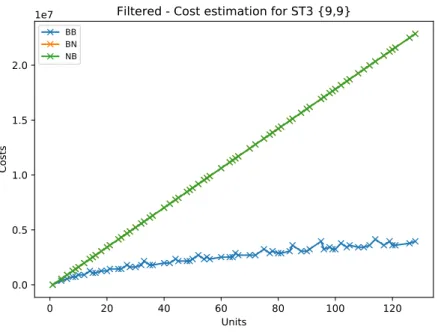
In Figure 4.3 the communication overhead of eachDASH pattern with increasing amount of units is shown with the three different stencils described in Table 5.3. Like mentioned earlier, every time theunits are a prime number the BB layout behaves like the NB layout, i.e. SOBB(d, s) =SON B(d, s).

Trough factorization of the numbers ofunits the derived equation becomes volatile. This violate behavior correlate to the R_S/V, R_H/W, see Figure 4.4. Therefore, the quantity of possible input units is limited in order to reduce the volatile behavior of the equation. If

units withRH/W > 1₄ are filtered out, only blocks with a more homogeneous ratio between

height and width remain which leads to a better R_S/V. In other words, the coefficient of variationvis minimized. A low coefficient of variation indicates a less volatile function. The variation without a filter isv_{nof ilter}2 = 0.96 whereas the variation using the described filter is reduced tov2_{nof ilter}= 0.42. From this it can be assumed that the best case for the count of

units is a square number. A square number on a square image will haveRH/W = 1.0. This

should result in the best performance for theBB pattern with an identical stencil inx and

y. A prime number ofunits should never be chosen, because in this case theBB layout will generate aunit decomposition with 1·u and this is similar to theNB layout. In Figure 4.5 the filtered function for ST3 is shown.

Figure 4.3 shows that the communication overhead over the network for ST1 with BN

pattern andST2 withNB pattern is 0. The reason for this is that there is no communication in the dimension which contains borders, so the calculation per unit is independent from other units.

(38)

Figure 4.3: SO(d, s) for the different patterns withST1,ST2 andST3. Assumed 100% brick locality while initialization. Right side the layout examples with the stencils to show alignment. Bottom plot: BN=NB.

0

20

40

60

80

100

120 Units/Cores

0.0

0.5

1.0

1.5

2.0

2.5 Costs

1e8

Estimation of cost devlopment for BB

ST(101,1) ST(1,101) ST(101,101)

(39)

4.3 Costfunction 0 20 40 60 80 100 120 Units 0.0 0.5 1.0 1.5 2.0 Costs

1e7

Filtered - Cost estimation for ST3 {9,9}

BB BN NB

Figure 4.5: FilteredSO(d, s) for the differentunits withST3. Assumed 100% brick locality while initialization. BN=NB.

(40)

4.4 Optimization Model

A given data distributiondoptis optimal if minimum of pixels is transferred over the network

for processing next distributiondnext with a given stencil s:

dopt=argmind∈{dA,dB,dC,dD,...}(C(d, dnext, s)) (4.8)

The next distributiondnext could be either of aBB,BN, orNB pattern. The initialization

phase should faster if more local bricks are available, so it should be useful to change the node order or manipulate theunit mapping to achieve a higher locality, or useunit pinning of the MPI framework. But this will result in a large amount of permutations, N it is N! and this already becomes large with a few nodes. For searching the global minimum it is no longer possible to calculate every solution in a reasonable time frame. In this problem space, other strategies have to be used. To reduce the permutations we can try to head for a local minimum. One strategy could be to just switch the first node with another and calculate if the locality is increasing for the patterns. If such a combination is found, we look at the second node and try to find again a combination with locality increase. This is repeated until each node is used for a search or as a change partner. At the end we only have to check n(n₂−1) permutations. But before putting effort into strategy, it is important to know if the effort to find this strategy will pay off. It is important to know how big the impact of inputting none local bricks vs. local bricks on the total performance of all processing steps is. Another possibility for optimization is to vary the amount ofunits, e.g. to gain a better RS/V and RH/W but this will result in a new initialization phase. One

advantage of not manipulating theunits is the ability to keep the data in memory and just change the patterns while processing. Anyway, writing back the intermediate results is a requirement for the RS processing to keep intermediate results for reuse in the future. So a new initialization phase could be possible, but only if the effect of a better ratio with less

units results in a performance gain and this have to be proofed in the experiments.

4.5 Optimization and Worker Software

The following section is a short overview of the implementation of the software framework for testing the optimization concept from the previous Chapter 3. The complete software stack is split in two layers. On the first layer is the Locality Optimizer for Remote Sensing Data, a Python program which analyzes the multi-channel SAR processing workflow and generates tasks as an output. The second software component is theRemote Sensing Image Distribute and Processor and is responsible for executing these tasks and is described in Section 4.5.2.

4.5.1 Locality Optimizer for Remote Sensing Data

For the implementation the Python version 3.7 created withAnacondaon anUbuntu 18.04.03 LTS operating system is used. The developed program’s task is to find the optimal distri-bution to speed up the given workflow for multi-channel remote sensing, see Figure 3.4. The input for the Locality Optimizer for Remote Sensing Data is a processing graph with multi-ple channel transformations and channel fusions at the end. Each fusion and transformation defines a stencil for the operation and uses a smoothing filter for workload simulation. After

Improving Data Locality in Distributed Processing of Multi-Channel Remote Sensing Data with Potentially Large Stencils

INSTITUT F ¨

UR INFORMATIK

Masterarbeit

Improving Data Locality in

Distributed Processing of

Multi-Channel Remote Sensing

Data with Potentially Large

Stencils

INSTITUT F ¨

UR INFORMATIK

Masterarbeit

Improving Data Locality in

Distributed Processing of

Multi-Channel Remote Sensing

Data with Potentially Large

Stencils

Philipp Patrick Posovszky

Contents

1 Introduction

1.1 Task and Definition of Goals

1.2 Structure

2 Processing of Large Scale Multi-Channel

Remote Sensing Data

2.1 Remote Sensing Images and Processing Images

2.2 Hardware Limitations

2.3 Distributed Computing

3 Distributed RS Image Processing

3.1 Problem Statement

3.2 Data Description

3.3 Stencil Computation

3.4 DASH - a PGAS Framework

3.5 Patterns in DASH

3.6 Multi-channel RS Processing Workflow

3.7 Brick and Data Locality

4 Optimization Model for Data Locality

4.1 Parameter Definition

b

b

b

b

b

b

b

b

b

b

b

b

b

b

b

b

4.2 Surface-to-volume and height-to-width Ratio

4.3 Costfunction

0

20

40

60

80

100

120

Units/Cores

0.0

0.5

1.0

1.5

2.0

2.5

Costs

1e8

Estimation of cost devlopment for BB

Filtered - Cost estimation for ST3 {9,9}

4.4 Optimization Model

4.5 Optimization and Worker Software