(will be inserted by the editor)
µ
JADE: Adaptive Differential Evolution with a Small Population
Craig Brown · Yaochu Jin · Matthew Leach · Martin Hodgson
Received: date / Accepted: date
Abstract This paper proposes a new differential evolution (DE) algorithm for unconstrained continuous optimisation problems, termedµJADE, that uses a small or ‘micro’ (µ) population. The main contribution of the proposed DE is a new mutation operator, ‘current-by-rand-to-pbest.’ With a population size less than 10,µJADE is able to solve some classical multimodal benchmark problems of 30 and 100 di-mensions as reliably as some state-of-the-art DE algorithms using conventionally sized populations. The algorithm also compares favourably to other small population DE variants and classical DE.
Keywords Micro differential evolution·Small Population· External Archive·JADE
1 Introduction
Differential Evolution (DE) (Storn and Price, 1997) is a deriva-tive free, population-based global optimisation algorithm. This work was funded by Bosch Thermotechnology Ltd. and the Engi-neering and Physical Sciences Research Council (EPSRC) UK.
C. Brown·M. Hodgson Bosch Thermotechnology Ltd. Worcester, Worcestershire, WR4 9SW, UK E-mail: [email protected] Y. Jin Department of Computing University of Surrey
Guildford, Surrey, GU2 7XH, UK E-mail: [email protected]
M.Leach
Centre for Environmental Strategy
Faculty of Engineering and Physical Sciences University of Surrey
Guildford, Surrey, GU2 7XH, UK E-mail: [email protected]
Its advantages are ease of use, ease of implementation and fast convergence. DE has enjoyed success in a range of ap-plications such as bioprocess optimisation and urban energy management among many more (Das and Suganthan, 2011). DE can also be used for on-line optimisation tasks aris-ing in control, notably nonlinear model predictive control (NMPC) (Yu et al, 2008). For DE to be practical as an opti-miser for NMPC, attention must be paid to the number of function evaluations that occur between time steps, espe-cially if the cost function is expensive to evaluate.
When applying DE to on-line optimisation problems, such as NMPC, it can be necessary to re-evaluate the pop-ulation if the optima move with time (Mendes and Mohais, 2005). Unfortunately, population based optimisation algo-rithms such as DE require large populations; the recomme-nded population sizeNPfor DE given a problem ofD di-mensions generally ranges from 2Dto 40D(Ronkkonen et al, 2005). For real-time use the computational cost of an itera-tion or populaitera-tion re-evaluaitera-tion could be restrictively large. Workarounds normally involve re-evaluating a subset of the population rather than the population in entirety. However, this approach may ignore promising search directions de-pending on how abruptly the fitness surface changes—it is desirable to re-evaluate the entire population between time steps.
For control applications, reliability of the optimisation is important: a poor solution could result in unacceptable plant behaviour. It is known that DE (typically) converges more quickly with smaller populations than with larger pop-ulations but at the cost of reduced reliability (Mallipeddi and Suganthan, 2008). However, the feasibility of using DE in embedded systems is improved by using small popula-tions—the memory requirement is reduced.
In view of the above considerations, µJADE is intro-duced. The idea is to acquire reliability comparable to that
of state-of-the-art DE but using a much smaller population than is commonly practised.
The rest of the paper is structured as follows. Firstly, an overview of classical DE, JADE (Zhang and Sanderson, 2009b) and Rcr-JADE (Gong et al, 2014) is given. Litera-ture relating to the use of small populations in DE is also reviewed.
Secondly, usingRcr-JADE as a foundation, µJADE is introduced. The modifications are described in Section 3 and the complete pseudocode is given in Algorithm 2.
Finally, µJADE is compared to three DE variants de-signed for small populations using a fixed small population size. It is then compared to 2 state-of-the-art DE algorithms that use a conventionally sized population:Rcr-JADE-s4 and FSADE (Sharma et al, 2014), as well as classical DE. Per-formance is compared in terms of function evaluations and success rate on some classical benchmarks at 30 dimensions. In addition,µJADE is compared toRcr-JADE-s4 at 100 di-mensions.
2 Related Work
This section is an overview of the original DE algorithm, its variants designed for small populations and a description of the adaptive DE variants JADE andRcr-JADE, on which µJADE is based.
2.1 Differential Evolution (DE)
DE is a method of solving optimisation problems of the form:
Minimise f(xxx), xxx∈ℜD (1)
whereDis the dimensionality of the optimisation problem andxxx= [x1,x2, ...,xd]T is the vector of decision variables. Each variablexjsatisfies a boundary constraint:
Lj≤xj≤Uj, j=1,2, ...,D, LLL∈ℜD, UUU∈ℜD (2) whereLjandUjare the lower and upper bound ofxj respec-tively.
There are 4 stages to DE. Firstly, a set of candidate so-lutions is created (initialisation). This set is called the popu-lation. Secondly, an operator is applied to each individual or target vector to create a mutant vector (mutation). Thirdly, another operator is applied to the target vector and the mu-tant vector to give a trial vector (crossover). Finally, a se-lection operation is used to determine which trial and target vectors are used in the next population. The last 3 stages are repeated until a satisfactory solution is found—each repeti-tion is called a generarepeti-tion.
2.1.1 Initialisation
Initially the populationP={xxx1,xxx2, ...,xxxNP}is generated ran-domly. The i’th vectorxxxi∈Pis initialised as follows:
xi,j=Lj+rand(0,1) (Uj−Lj) (3)
where rand(0,1) is drawn from a uniform distribution in (0,1),i=1,2, ...NPand j=1,2, ...,D.
2.1.2 Mutation
A mutation operator is applied to each target vectorxxxi. The classical mutation operator denoted DE/rand/1 is as follows:
vvvi=xxxa+F(xxxb−xxxc) (4)
wherei,a,b,c∈ {1,2, ...,NP}andi6=a6=b6=c.
Often it is important that the bounds of the problem aren’t violated by the mutation operation. One scheme for ensuring this is given in Zhang and Sanderson (2009b):
vi,j= (Lj+xi,j) 2 ifvi,j<Lj (Uj+xi,j) 2 ifvi,j>Uj vi,jotherwise (5) 2.1.3 Crossover
Following mutation, a crossover operator is applied to each target vectorxxxiand its associated mutant vectorvvvito give a trial vectoruuui. A popular crossover operator is the binomial crossover: ui,j= ( vi,j if OR(rand(0,1)<CR,j=jrand) xi,j otherwise (6)
whereCR∈[0,1]and jrand∈ {1,2, ...,D}and is randomly selected.
2.1.4 Selection
Finally, the selection operation replaces members of the pop-ulation with the corresponding trial vector if the trial vector has a better fitness.
xxxi=
(
uuui if f(uuui)<f(xxxi)
xxxi otherwise
(7)
wheref(xxx)is the objective function to be optimised. An alternative approach is to replace the target vector with the trial vector if the trial vector has a better or equal fit-ness. In the case that the population lies entirely on a plateau it keeps moving as long as the population is not identical.
This is useful for small populations where firstly, this sce-nario is more likely and secondly, the number of possible outcomes per mutation and target vector is smaller (moving the population creates new mutation possibilities even if it does not improve the fitness). Contrast this to the former se-lection method where the population will remain stationary on a plateau unless a fitness improvement can be made—the number of possible trial vectors is relatively limited. This in-creases the risk of stagnation (Lampinen and Zelinka, 2000).
xxxi= ( u u ui if f(uuui)≤f(xxxi) xxxi otherwise (8) 2.2 Small populations in DE
Mallipeddi and Suganthan (2008) carried out a study of the effects of population size on DE using 2 mutation opera-tors, DE/best/1 and DE/rand to best/2, withNPranging from 2Dto 10D. They concluded that smaller populations with greedy mutation strategies converge quickly but are more likely to stagnate or converge prematurely. Conversely, a large population with an exploratory mutation operator sig-nificantly reduces the probability of this happening at the cost of slower convergence.
Ren et al (2010) developed a new mutation operator for smaller population sizes in DE. They were able to solve some 30 dimensional test problems using a population size as low as 5. They added a random disturbance to DE/rand/ 1/bin:
vvvi=xxxa+F(xxxb−xxxc+rand(−1,1)δδδ) (9) where rand(−1,1)generates a random number in the inter-val (-1,1) andδδδis a function of the fraction of the population
IRthat improves at each generation:
δ δδ(IR) = δ δδ η ifIR<0.2 δ δδ η ifIR>0.2 δ δδ otherwise (10)
whereδδδ is initialised as follows:
δj=α(Uj−Lj) (11)
whereα is a constant.
Brest and Mauˇcec (2011) made use of the different be-haviour of small and large populations with different muta-tion operators in their jDEl-scop algorithm. The algorithm uses an adaptive population size, adaptive Fi andCRi and an ensemble of mutation and crossover strategies. Using a
starting population size of 100, they were able to consis-tently solve some benchmark functions atD=200,D=500 andD=1000. Some other adaptive population schemes are given in Teo (2006), Teng et al (2009), Wang and Zhao (2013), Yang et al (2013), Zhao et al (2014) and Choi and Ahn (2014).
Fajfar et al (2012) investigated population sizes as low as 10 for a set ofD=30 benchmark problems. They combined random perturbation of the trial vector (Equation 12) with a new selection operation (Algorithm 1) to improve the formance of DE/rand/1/bin, with the improvement of per-formance most pronounced at low population sizes. The se-lection operation works by allowing each trial vector to be compared to each target vector and to the first half of the population sequentially. If the fitness function is improved compared to the population vector, that vector is replaced by the trial vector and the selection process is restarted for the next target vector.
ui,j=
(
Lj+rand(0,1)×(Uj−Lj) if rand(0,1)≤0.005
ui,j otherwise
(12)
Algorithm 1:Selection operation of Fajfar et al (2012) 1 iff(uuui)<f(xxxi)then 2 c=i 3 else 4 c=−1 5 forp=1toNP2 do 6 iff(uuui)<f(xxxp)then 7 c=p 8 exit loop 9 ifc6=−1then 10 xxxc=uuui
Salehinejad et al (2014) increased the diversity of the population in small population DE by vectorising the scal-ing factor,Fi. Rather thanFi being a scalar for each target vector,FFFiis a vector of length D and each element is drawn from a uniform distribution in (0.1, 1.5) for each population member. The mutation becomes:
vvvi,j=xxxa,j+Fi,j(xxxb,j−xxxc,j) (13) wherej=1,2, ...,D.
In summary, the literature indicates that the performance of DE at small populations can be improved using the right modifications. Perturbation appears an important theme. Im-proving the number of possible trial vectors is also impor-tant—Salehinejad et al (2014) achieved this by randomising
the scaling factor for each individual and each dimension. The main difficulty in using small populations in DE is over-coming their limited exploration ability. Selection may also be an important area of enquiry that has received little atten-tion in the literature so far (Fajfar et al, 2011).
A distinct but related field in DE is compact DE (cDE) (Mininno et al, 2011). In cDE, the population is replaced by a statistical representation whose memory requirement is equivalent to a population of 4 individuals regardless of the dimensionality of the problem, though the search behaves as if the population were larger due to the randomised creation of individuals at each iteration. Compact DE is not investi-gated here—the emphasis of this paper is on using DE with small non-virtual populations.
2.3 JADE: Adaptive Differential Evolution
Zhang and Sanderson (2009b) introduced an adaptive DE variant called JADE with an optional external archive for conventionally sized populations. The archive contains pre-vious population members that had been replaced by a trial vector. The relevance of the archive to small populations is that there will be a larger set of possible outcomes for a given trial vector as if the population were larger—a higher num-ber of possible trial outcomes lowers the risk of the popula-tion stagnating (Lampinen and Zelinka, 2000). The mutapopula-tion operator for JADE, denoted DE/current-to-pbest/1, without an external archive is:
vvvi=xxxi+Fi(xxxbestp −xxxi) +Fi(xxxa−xxxb) (14) wherexxxpbest is randomly chosen from the top 100p% pop-ulation members. The mutation for JADE with an external archive is:
vvvi=xxxi+Fi(xxxbestp −xxxi) +Fi(xxxa−xxx˜b) (15) where ˜xxxb is randomly chosen fromP∪A. The effect is to improve the diversity of the population.
Alternatively, DE/rand-to-pbest/1, introduced by Zhang and Sanderson (2009a), is:
vvvi=xxxa+Fi(xxxpbest−xxxa) +Fi(xxxb−xxxc) (16) and with archive:
vvvi=xxxa+Fi(xxxpbest−xxxa) +Fi(xxxb−xxx˜c) (17) where ˜xxxcis randomly chosen fromP∪A.
Following the mutation step, JADE uses the binomial crossover operator given in Equation 6 and the selection op-eration given in Equation 7.
In JADE,Fi andCRi are randomly generated at the be-ginning of each generation according to:
CRi=randni(µCR,0.1); (18)
Fi=randci(µF,0.1); (19)
whereCRiis drawn from a normal distribution of meanµCR and standard deviation 0.1 andFi is drawn from a Cauchy distribution of location parameterµF and scale factor 0.1. As long asFi≤0 it is redrawn from the distribution. IfFi>1 it is truncated to 1.CRis truncated to [0, 1]. At the end of each generationµCRandµFare updated as follows:
µCR= (1−c)µCR+c·L1(Scr) (20) µF= (1−c)µF+c·L2(SF) (21) whereScr is the set of successfulCR values in the current generation,SFis the set of successfulFvalues in the current generation and: Lp({z1,z2, ...zn}) = ∑nk=1z p k ∑nk=1z p−1 k (22) 2.4Rcr-JADE
As discussed in Section 2.3, JADE uses an adaptiveCRand
F scheme. Gong et al (2014) introduced a modification to JADE wherebyCRis corrected at each generation based on the actual crossover rate a posteriori. The crossover opera-tion becomes:
di,j=rand(0,1) (23)
ui,j=
(
vi,j if OR(di,j<CRi,j=jrand)
xi,j otherwise
(24)
bi,j=
(
1 if OR(di,j<CRi,j=jrand)
0 otherwise (25)
CRi=
∑Dj=1bi,j
D (26)
Another change from JADE is thatRcr-JADE uses the selection operation given in Equation 8 rather than that of Equation 7.
3 ModifyingRcr-JADE for small populations:µJADE In this section, four modifications toRcr-JADE intended sp-ecifically for use with small populations are introduced. The aim is to retain the desirable property of small populations, that is, fast convergence, whilst improving the robustness, which is typically associated with larger populations.
DE with small populations is known as µDE or micro DE. Therefore, the new algorithm is denotedµJADE, to in-dicate both its origin and its suitability to small populations.
3.1 New mutation operator forRcr-JADE
A new mutation operator is introduced denoted current-by-rand-to-pbest/1:
vvvi=xxxi+Fi(xxxbestp −xxxa) +Fi(xxxb−xxx˜c) (27) where ˜xxxcis randomly chosen fromP∪A. The idea of the mu-tation is to improve the exploratory power of small popula-tions whilst retaining good convergence performance. When
xxxi6≈xxxa andxxxi 6=xxxa, current-by-rand-to-pbest/1 is explor-atory. However, whenxxxi≈xxxa, current-by-rand-to-pbest/1 is similar to current-to-pbest/1. The latter is more likely as the population and archive converges. The aim is to accelerate convergence in the later stages of optimisation and reduce the likelihood of the population accumulating at a false op-timum in the early stages of optimisation.
Conventionally in JADE, ˜xxxc 6=xxxb and ˜xxxc6=xxxa. These constraints are removed forµJADE. Instead, the constraint
xxxpbest6=xxxais upheld. Then, when ˜xxxc=xxxbandxxxi≈xxxa, the mu-tation is greedy. The constraintxxxa6=xxxbis upheld to prevent the second displacement term reversing the first ifxxxbestp =xxx˜c andxxxb=xxxa.
3.2 Changes toF andCRadaptation
In JADE andRcr-JADEµCRandµFare updated every gener-ation according to Equgener-ations 20 and 21 respectively. As long asScr=/0,CRdecays at each generation. Similarly, as long asSF=/0,µFdecays at each generation. For small popula-tions, the probability of achieving a successful trial vector at each generation is lower than for large populations, re-sulting inFandCRvalues quickly diminishing. Put another way, the sample size of successfulF andCR values is not large enough to give reliable estimates forµFandµCR.
In order to solve this,µJADE updatesµCR andµF ev-ery max(100,10D)generations rather than every 1 genera-tion. The lower limit, 100, through trial and error was found to perform reasonably. This modification can cause the sets
SCR andSF to become very large. Therefore, it is recom-mended to calculateµF andµCRrecursively in practice.
3.3 Perturbation
In order to give µJADE a chance of escaping false optima and improve diversity, the perturbation method of Fajfar et al (2012) is incorporated intoµJADE after crossover. To incor-porate this perturbation mechanism without disrupting the crossover repair introduced by Gong et al (2014),biis rected after the perturbation step before calculating the cor-rected crossover: ri,j=rand(0,1) (28) ui,j= ( Lj+rand(0,1)(Uj−Lj) ifri,j≤0.005 ui,j otherwise (29) bi,j= ( 0 ifri,j≤0.005 bi,j otherwise (30) 3.4 Restart
As an ‘insurance’ for the worst case scenario where the best fitness stagnates despite the aforementioned modifications, the population (excluding the best member) is re-initialised if the best fitness doesn’t improve for max(1000,100D) gen-erations.
4 Experimental Setup
µJADE is first compared to some small population DE vari-ants for problems of 30 dimensions. Experimentally, it was found that 8 is the smallest population with whichµJADE works effectively. In order to compare to other small popu-lation DE variants, a fixed popupopu-lation size of 8 is also used. The population size is fixed across all the variants since even a small difference in population size is proportionally signif-icant when using very small populations.
Firstly, the small population algorithms DESP (Ren et al, 2010), MDEVM (Salehinejad et al, 2014) and MDEVM with the perturbation and selection modifications of Fajfar et al (2012) (denoted MDEVM-Fajfar) are compared (we found this combination to perform better than DE/rand/1/bin-Fajfar). As DESP, MDEVM and MDEVM-Fajfar are closely related to DE/rand/1/bin and use static parameters, the standard set-ting ofCR=0.9 is used. Additionally,F =0.5 for DESP and DE/rand/bin/1 (Montgomery and Chen, 2010; Zhang and Sanderson, 2009b). Otherwise, DESP uses the param-eter settings given in Ren et al (2010).
ForµJADE, only the value forpdiffers from that speci-fied by Zhang and Sanderson (2009b); in the original JADE algorithm p=0.05 which is too small for the population sizes used inµJADE (pNPshould be an integer greater than 1). Therefore, forµJADEp=3/NP.
µJADE is then compared to some state-of-the-art DE variants that use conventionally sized populations—rcr -JADE-s4 (Gong et al, 2014) and FSADE (Sharma et al, 2014). µJADE is also compared to DE/rand/1/bin. ForRcr -JADE-s4,µF=0.5,µCR=0.5,p=0.05,c=0.1 andNP=100,400 forD=30,100 respectively (Zhang and Sanderson, 2009b; Gong et al, 2014). For FSADE the settings given in Sharma et al (2014) are used.
In addition, the mutations rand-to-pbest/1 and current-by-rand-to-pbest/1 are compared inµJADE for a small fixed number of function evaluations.
Algorithm 2:µJADE 1 Initialise population 2 µCR=0.5
3 µF=0.5 4 A=/0
5 forg=1 to number of generationsdo 6 for i=1 toNPdo
7 CRi=randni(µCR,0.1) 8 Fi=randci(µF,0.1) 9 Randomly selectxxxa6=xxxi 10 Randomly selectxxxb6=xxxa6=xxxi
11 Randomly selectxxxbestp 6=xxxafrompNPbest population members
12 Randomly selectxxxcfromP∪A 13 Randomly selectjrand∈N+≤D
/* Mutation */ 14 vvvi=xxxi+Fi(xxx p best−xxxa) +Fi(xxxb−xxx˜c) 15 vi,j= (Lj+xi,j) 2 ifvi,j<Lj (Uj+xi,j) 2 ifvi,j>Uj vi,jotherwise /* Crossover */ 16 forj=1 toDdo 17 di,j=rand(0,1) 18 ui,j= ( vi,j if OR(di,j<CRi,j=jrand) xi,j otherwise 19 bi,j= ( 1 if OR(di,j<CRi,j=jrand) 0 otherwise /* Perturbation */ 20 forj=1 toDdo 21 ri,j=rand(0,1) 22 ui,j= ( Lj+rand(0,1)(Uj−Lj)ifri,j≤0.005 ui,j otherwise 23 bi,j= ( 0 ifri,j≤0.005 bi,j otherwise /* Crossover Repair */ 24 CRi= ∑Dj=1bi,j D /* Selection */ 25 iff(uuui)≤f(xxxi)then 26 xxxi→A 27 xxxi=uuui 28 CRi→SCR 29 Fi→SF
30 ifuuuiis fitter than best population memberthen 31 BIR=BIR+1
/* Archive Update */
32 Randomly remove solutions fromAso that|A| ≤NP
/* Parameter Update */ 33 ifmod(g,max(100,10D) = 0then 34 µCR= (1−c)µCR+cL1(SCR)// L1(/0) =0 35 µF= (1−c)µF+cL2(SF)// L2(/0) =0 36 SCR=SF=/0 /* Reset */ 37 ifmod(g,max(1000,100D) = 0then 38 ifBIR=0then
39 Reinitialise population apart from best member 40 BIR=0
In this work, all variants apply Equation 5 after the mu-tation to prevent bounds violation.
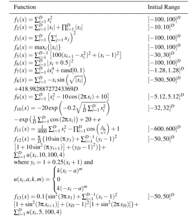
The scalable benchmark functions are given in Table 1. Respectively, they are known as the Sphere, Schwefel 2.22, Schwefel 1.2, Schwefel 2.21, Rosenbrock, Step, Noisy Quar-tic, Schwefel 2.26, Rastringin, Ackley, Griewank, and the two Generalized Penalty Functions (Yao et al, 1999).
The comparisons are made in terms of success rate and number of function evaluations required to achieve a solu-tion accuracy of less than 1.0e-02 for f7 and 1.0e-08 for all other functions. If the required solution accuracy isn’t achieved after 100000Dfunction evaluations the run is con-sidered unsuccessful. This large number of function evalu-ations ensures the algorithms are tested to exhaustion, em-phasising reliability over convergence speed.
Table 1 Benchmark Functions (Yao et al, 1999)
Function Initial Range
f1(x) =∑Di=1xi2 [−100,100]D f2(x) =∑Di=1|xi|+∏Di=1|xi| [−10,10]D f3(x) =∑Di=1 ∑ij=1xj 2 [−100,100]D f4(x) =maxi{|xi|} [−100,100]D f5(x) =∑Di=−11 100(xi+1−xi2)2+ (xi−1)2 [−30,30]D f6(x) =∑Di=1bxi+0.5c2 [−100,100]D f7(x) =∑Di=1ix4i+rand[0,1) [−1.28,1.28] D f8(x) =∑Di=1−xisin p |xi| [−500,500]D +418.98288727243369D f9(x) =∑Di=1 x2 i−10 cos(2πxi) +10 [−5.12,5.12]D f10(x) =−20 exp −0.2 q 1 D∑ D i=1x2i [−32,32]D −exp 1 D∑ D i=1cos(2πxi) +20+e f11(x) =40001 ∑ D i=1x2i−∏Di=1cos xi √ i +1 [−600,600]D f12(x) =π D{10 sin(πy1) +∑ D−1 i=1 (yi−1)2 [−50,50]D 1+10 sin2(πyi+1) + (yD−1)2)}+ ∑Di=1u(xi,10,100,4) whereyi=1+0.25(xi+1)and u(xi,a,k,m) = k(xi−a)m 0 k(−xi−a)m f13(x) =0.1{sin2(3 πx1) +∑Di=−11(xi−1)2 [−50,50]D [1+sin2(3πxi+1)] + (xD−1)2[1+sin2(2πxD)]}+ ∑Di=1u(xi,5,100,4)
5 Experimental Results and Analysis
Table 2 shows the Success Rate (SR) and mean number of Function Evaluations (FE) in successful runs of MDEVM-Fajfar, MDEVM, DESP andµJADE in the 30 dimensional test problems.µJADE is clearly the most reliable small pop-ulation algorithm overall.
DESP performs poorly across most of the benchmarks. In DESP, individuals will be more greatly perturbed as CR increases because the perturbation is incorporated into the
Table 2 Comparison of small population algorithms for D = 30. Mean over 50 independent runs. Best results are in boldface and are ranked first by reliability then by convergance speed (Wilcoxonα=0.05)
f MDEVM-FajfarNP=8 MDEVMNP=8 DESPNP=8 µJADENP=8
SR(%) FE’s Mean (Std) SR(%) FE’s Mean (Std) SR(%) FE’s Mean (Std) SR(%) FE’s Mean (Std)
f1 98 8.6e+04 (4.1e+05) 100 2.8e+04 (3.3e+03) 100 1.9e+04(8.0e+02) 100 2.2e+04 (7.8e+02)
f2 86 6.0e+04 (1.5e+05) 100 3.1e+04(4.7e+03) 0 — 100 3.7e+04 (1.2e+03)
f3 54 3.4e+05 (4.7e+05) 100 1.4e+05(1.5e+04) 0 — 100 1.6e+05 (7.7e+03)
f4 0 — 0 — 0 — 100 2.2e+05 (1.6e+04)
f5 0 — 52 2.3e+06 (4.0e+05) 0 — 98 2.1e+05 (5.5e+04)
f6 100 4.1e+05 (3.1e+05) 100 1.8e+04 (6.3e+03) 0 — 100 1.2e+04(3.8e+03)
f7 100 3.4e+05 (2.2e+05) 76 8.9e+05 (7.1e+05) 0 — 100 2.3e+05(1.6e+05)
f8 96 6.9e+04 (1.6e+05) 0 — 0 — 100 1.0e+05 (5.1e+03)
f9 90 1.6e+05 (4.0e+05) 0 — 0 — 100 1.2e+05 (6.8e+03)
f10 70 9.5e+04 (1.0e+05) 0 — 0 — 100 3.8e+04 (5.0e+03)
f11 24 4.0e+04 (4.7e+04) 20 2.6e+04 (3.1e+03) 50 3.1e+04 (1.7e+03) 100 4.6e+04 (3.7e+04)
f12 100 9.5e+04 (2.3e+05) 40 6.6e+04 (6.5e+04) 2 1.8e+06 (0.0e+00) 100 3.8e+04 (7.5e+03)
f13 92 4.2e+05 (6.8e+05) 32 7.0e+04 (6.4e+04) 0 — 100 3.2e+04 (1.8e+04)
70 48 12 99.85
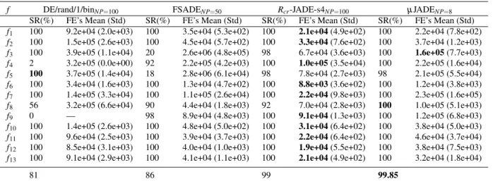
Table 3 Comparison for D = 30. Mean over 50 independent runs.
f DE/rand/1/binNP=100 FSADENP=50 Rcr-JADE-s4NP=100 µJADENP=8
SR(%) FE’s Mean (Std) SR(%) FE’s Mean (Std) SR(%) FE’s Mean (Std) SR(%) FE’s Mean (Std)
f1 100 9.2e+04 (2.0e+03) 100 3.5e+04 (5.3e+02) 100 2.1e+04(4.9e+02) 100 2.2e+04 (7.8e+02)
f2 100 1.5e+05 (2.6e+03) 100 4.5e+04 (5.7e+02) 100 3.3e+04(7.6e+02) 100 3.7e+04 (1.2e+03)
f3 100 3.9e+05 (1.1e+04) 20 2.6e+06 (4.8e+05) 98 6.7e+04 (3.6e+03) 100 1.6e+05(7.7e+03)
f4 2 3.2e+05 (0.0e+00) 92 2.2e+05 (4.2e+03) 100 1.0e+05(3.5e+04) 100 2.2e+05 (1.6e+04)
f5 100 3.7e+05 (1.4e+04) 18 2.8e+06 (6.1e+04) 98 7.8e+04 (2.7e+03) 98 2.1e+05 (5.5e+04)
f6 100 3.4e+04 (1.6e+03) 100 1.3e+04 (4.7e+02) 100 8.8e+03(3.6e+02) 100 1.2e+04 (3.8e+03)
f7 100 1.4e+05 (3.3e+04) 100 1.1e+05 (2.6e+04) 100 2.2e+04(9.8e+03) 100 2.3e+05 (1.6e+05)
f8 56 3.2e+05 (6.6e+04) 90 4.4e+04 (1.8e+03) 92 7.0e+04 (2.8e+03) 100 1.0e+05 (5.1e+03)
f9 0 — 98 8.9e+04 (4.8e+03) 100 9.1e+04(1.3e+03) 100 1.2e+05 (6.8e+03)
f10 100 1.4e+05 (2.6e+03) 100 4.8e+04 (5.0e+02) 100 3.1e+04(6.4e+02) 100 3.8e+04 (5.0e+03)
f11 100 9.6e+04 (2.5e+03) 100 3.9e+04 (3.7e+03) 100 2.2e+04(6.4e+02) 100 4.6e+04 (3.7e+04)
f12 100 8.5e+04 (3.1e+03) 100 4.0e+04 (1.0e+03) 100 1.9e+04(5.5e+02) 100 3.8e+04 (7.5e+03)
f13 100 9.1e+04 (2.9e+03) 100 4.1e+04 (1.1e+03) 100 2.1e+04(4.9e+02) 100 3.2e+04 (1.8e+04)
81 86 99 99.85
Table 4 Comparison of the mutation operators forD=30,NP=8.
Mean fitness after 3e+04 function evaluations over 50 independent runs.
f current-by-rand-to-pbest/1 rand-to-pbest/1
f(xxx)Mean (Std) f(xxx)Mean (Std)
f1 9.0e-13(2.5e-12) 5.3e-01 (9.5e-01)
f2 1.3e-06(1.6e-06) 1.2e-01 (8.2e-02)
f3 9.7e+02(4.2e+02) 2.6e+03 (1.4e+03)
f4 4.9e+00(2.5e+00) 1.1e+01 (1.7e+00)
f5 4.3e+01(2.9e+01) 6.2e+02 (7.0e+02)
f6 2.0e-02(1.4e-01) 2.8e+00 (3.1e+00)
f7 4.6e-02(1.4e-02) 1.1e-01 (5.2e-02)
f8 4.0e+03 (4.5e+02) 3.4e+00(6.5e+00)
f9 1.2e+02 (1.4e+01) 2.8e+00(1.4e+00)
f10 2.3e-02(1.6e-01) 1.1e+00 (5.4e-01)
f11 2.1e-03(4.8e-03) 4.5e-01 (3.0e-01)
f12 3.2e-01 (6.1e-01) 9.4e-03(2.8e-02)
f13 2.6e-03(1.4e-02) 5.2e-02 (7.3e-02)
mutation. High values ofCR, normally recommended for solving nonseparable problems, will cause a higher degree
of perturbation in DESP. In contrast, Fajfar-MDEVM and µJADE apply perturbation after selection and independently ofCR. Using aCRvalue of 0.9 will cause DESP to rely much more on perturbation than Fajfar-MDEVM andµJADE. Ren et al (2010) usedCRvalues as low as 0.05 for some prob-lems. This may explain the poor performance observed in this study. The algorithm may benefit from a pool of mu-tations with differentCR andF parameters similar to that described in Wang et al (2011).
Another observation is that MDEVM-Fajfar generally outperforms MDEVM. Especially on the multimodal func-tions, the modifications of Fajfar et al (2012) strongly benefit its performance. However, the performance on some of the unimodal benchmarks deteriorates.
Table 3 shows the comparison ofµJADE to DE variants that use much larger populations.µJADE compares favour-ably to FSADE and DE/rand/1/bin both in terms of reliabil-ity and convergence speed. It is slightly more reliable than
Table 5 Comparison for D = 100. Mean over 50 independent runs.
f Rcr-JADE-s4NP=400 µJADENP=8
SR(%) FE’s Mean (Std) SR(%) FE’s Mean (Std)
f1 100 1.1e+05(1.2e+03) 100 1.5e+05 (7.1e+03)
f2 100 1.7e+05(1.8e+03) 100 2.1e+05 (1.4e+04)
f3 94 9.3e+05 (3.1e+04) 100 2.5e+06 (1.3e+05)
f4 0 — 100 6.6e+06 (1.0e+05)
f5 100 8.3e+05(1.6e+04) 100 2.1e+06 (8.4e+05)
f6 100 4.6e+04(6.6e+02) 100 2.1e+05 (7.9e+04)
f7 100 1.3e+05 (1.4e+04) 28 7.0e+06 (2.4e+06)
f8 100 8.7e+05 (1.3e+04) 100 5.6e+05(7.4e+04)
f9 100 1.1e+06 (7.5e+03) 100 8.4e+05(1.3e+05)
f10 100 1.6e+05(1.6e+03) 100 2.7e+05 (1.6e+04)
f11 100 1.1e+05(1.3e+03) 100 3.5e+05 (2.5e+05)
f12 98 9.5e+04 (1.3e+03) 100 4.0e+05 (7.8e+04)
f13 98 1.1e+05 (1.3e+03) 100 2.2e+05 (6.0e+04)
92 95
Rcr-JADE-s4 overall. However,µJADE is generally slower thanRcr-JADE-s4 on successful runs.
Generally,µJADE and the other small population vari-ants show greater variance in the number of function eval-uations on successful runs. Larger populations sample the fitness landscape more thoroughly following initialisation compared to smaller ones. This may explain the superior consistency of the DE algorithms using larger populations observed in this study.
The restart mechanism can increase the variance of func-tion evaluafunc-tions to solve a given problem. Waiting for 1 restart will add max(1000,100D)function evaluations. Rest-arts are more likely on multimodal problems that cause pre-mature convergence above the error threshold.
The progress in median fitness ofµJADE and classical DE over the nonseparable Rosenbrock function at 30 di-mensions is shown in Figure 1. The former shows greater interquartile range as indicated by the wider grey band. In contrast, for the Ackley function (Figure 2), both algorithms show a comparable interquartile range. This may be because µJADE is more sensitive to the initial population for the Rosenbrock function than for the Ackley function. Popula-tion initialisaPopula-tion and re-initialisaPopula-tion could be an important avenue of further enquiry for using small populations more effectively (Kazimipour et al, 2014).
Table 4 shows the performance difference betweenµJADE with current-by-rand-to-pbest/1 and µJADE with rand-to-pbest/1 for a population size of 8. It can be seen that much of the performance ofµJADE can be attributed to the new mutation operator.
ForD=100, µJADE and Rcr-JADE-s4 are compared. The results are given in Table 5. µJADE is of comparable reliability toRcr-JADE-s4 on the majority of problems de-spite the large difference in population size. The new mu-tation, current-by-rand-to-pbest/1 is exploratory in the early stages of optimisation:xxxi, in the most part, is displaced by
Function Evaluations Fitness 0.5 1 1.5 2 x 10⁵ 10−10 10−5 100 105 µJADENP=8 DE/rand/1/binNP=100
Fig. 1 Convergence plots of the median fitness for the Rosenbrock
function at 30 dimensions. The grey shaded regions are bounded by the upper and lower quartile
Function Evaluations Fitness 0.5 1 1.5 2 x 10⁵ 10−15 10−10 10−5 100 µJADENP=8 DE/rand/1/binNP=100
Fig. 2 Convergence plots of the median fitness for the Ackley function at 30 dimensions. The grey shaded regions are bounded by the upper and lower quartile
difference vectors calculated independently ofxxxi. This en-ablesµJADE to be competitive even on multimodal optimi-sation problems as it can spend many generations exploring before showing greedier behaviour. Moreover, as perturba-tion occurs independently ofCR, the parameter adaptation mechanism can work unhindered. However, the noisy
quar-tic function f7causesµJADE to converge extremely slowly and often not within the 100000Dfunction evaluation limit. Interestingly,Rcr-JADE-s4 is unable to solvef4whereas the original JADE with archive is (Zhang and Sanderson, 2009b).Rcr-JADE uses the selection operation given in Equa-tion 8 rather than EquaEqua-tion 7 used in JADE. Since f4 is only concerned with the maximum value in |xxxi|, the con-dition f(xxxi) =f(uuui)will occur frequently. It is possible that Equation 8 causes Rcr-JADE-s4 to behave too greedily in the absence of a fitness improvements. ThoughµJADE also uses the selection operation given in Equation 8, it is not necessarily greedy as discussed in Section 3.1.
6 Conclusion
DE with a small population, or micro DE, is useful for dy-namic and resource constrained optimisation tasks. This pa-per presented a new DE algorithm,µJADE, that despite us-ing a population size much smaller than the number of de-cision variables, is more reliable than some state-of-the-art DE algorithms using conventionally sized populations. Our results indicate that small population DE has a promising future.
In this paper the classical benchmark functions were used to testµJADE. Further work is needed to determine whether the same reliability can be achieved for more difficult bench-mark problems, such as those that are shifted and rotated and dynamic optimisation benchmarks. In addition, due to its ap-parent reliability with a small population size,µJADE could be a suitable algorithm for incorporation into a cooperative coevolution scheme for large scale optimisation.
Acknowledgements The authors would like to thank the anonymous
reviewers for helping to improve this paper.
References
Brest J, Mauˇcec M (2011) Self-adaptive differential evolu-tion algorithm using populaevolu-tion size reducevolu-tion and three strategies. Soft Comput 15:2157–2174
Choi T, Ahn C (2014) An adaptive differential evolution al-gorithm with automatic population resizing for global nu-merical optimization. In: Pan L, Pˇaun G, P´erez-Jim´enez M, Song T (eds) Bio-Inspired Computing—Theories and Applications, Communications in Computer and Infor-mation Science, vol 472, Springer, pp 68–72
Das S, Suganthan P (2011) Differential evolution: A survey of the state-of-the-art. IEEE Trans on Evolutionary Com-put 15:4–31
Fajfar I, Puhan J, Tomaˇziˇc S, B˝urmen A (2011) On selection in differential evolution. Elektrotehniˇski Vestnik 78:275– 280
Fajfar I, Tuma T, Puhan J, Olenˇsek J, B˝urmen A (2012) To-wards smaller populations in differential evolution. J of Microelectron, Electron Compon and Materials 42:152– 163
Gong W, Cai Z, Wang Y (2014) Repairing the crossover rate in adaptive differential evolution. Appl Soft Comput 15:149–168
Kazimipour B, Li X, Qin A (2014) Effects of population initialization on differential evolution for large scale opti-mization. In: 2014 IEEE Congress on Evolutionary Com-putation, pp 2404–2411
Lampinen J, Zelinka I (2000) On stagnation of the differen-tial evolution algorithm. In: 6th International Conference on Soft Computing MENDEL, pp 76–83
Mallipeddi R, Suganthan P (2008) Empirical study on the effect of population size on differential evolution algo-rithm. In: The 2008 IEEE Congress on Evolutionary Computation, pp 3663–3670
Mendes R, Mohais A (2005) DynDE: a differential evolu-tion for dynamic optimizaevolu-tion problems. In: The 2005 IEEE Congress on Evolutionary Computation, vol 3, pp 2808–2815
Mininno E, Neri F, Cupertino F, Naso D (2011) Com-pact differential evolution. IEEE Trans on Evol Comput 15:32–54
Montgomery J, Chen S (2010) An analysis of the operation of differential evolution at high and low crossover rates. In: 2010 IEEE Congress on Evolutionary Computation, pp 1–8
Ren X, Chen Z, Ma Z (2010) Differential evolution using smaller population. In: 2010 Second International Con-ference on Machine Learning and Computing, pp 76–80 Ronkkonen J, Kukkonen S, Price K (2005) Real-parameter
optimization with differential evolution. In: The 2005 IEEE Congress on Evolutionary Computation, vol 1, pp 506–513
Salehinejad H, Rahnamayan S, Tizhoosh H, Chen S (2014) Micro-differential evolution with vectorized random mu-tation factor. In: 2014 IEEE Congress on Evolutionary Computation, pp 2055–2062
Sharma H, Shrivastava P, Bansal J, Tiwari R (2014) Fitness based self adaptive differential evolution. In: Terrazas G, Otero F, Masagosa A (eds) Nature Inspired Cooperative Strategies for Optimization (NICSO 2013), Studies in Computational Intelligence, vol 512, Springer, pp 71–84 Storn R, Price K (1997) Differential evolution—a simple
and efficient heuristic for global optimization over con-tinuous spaces. J of Glob Optim 11:341–359
Teng N, Teo J, Hijazi M (2009) Self-adaptive population sizing for a tune-free differential evolution. Soft Comput 13:709–724
Teo J (2006) Exploring dynamic self-adaptive populations in differential evolution. Soft Comput 10:673–686
Wang X, Zhao S (2013) Differential evolution algorithm with self-adaptive population resizing mechanism. Math Probl in Eng 2013, Article ID 419372
Wang Y, Cai Z, Zhang Q (2011) Differential evolution with composite trial vector generation strategies and control parameters. IEEE Trans on Evol Comput 15:55–66 Yang M, Cai Z, Li C, Guan J (2013) An improved adaptive
differential evolution algorithm with population adapta-tion. In: Proceedings of the 15th Annual Conference on Genetic and Evolutionary Computation, pp 145–152 Yao X, Liu Y, Lin G (1999) Evolutionary programming
made faster. IEEE Trans on Evol Comput 3:82–102 Yu X, Huang D, Wang X, Jin Y (2008) DE-based neural
net-work nonlinear model predictive control and its applica-tion for the pH neutralizaapplica-tion reactor control. In: Chinese Control and Decision Conference 2008, pp 1597–1602 Zhang J, Sanderson A (2009a) Adaptive Differential
Evo-lution: A Robust Approach to Multimodal Problem Optimization. Adaptation, Learning and Optimization, Springer, Berlin
Zhang J, Sanderson A (2009b) JADE: Adaptive differential evolution with optional external archive. IEEE Trans on Evolutionary Comput 13:945–958
Zhao S, Wang X, Chen L, Zhu W (2014) A novel self-adaptive differential evolution algorithm with population size adjustment scheme. Arab J for Science and Eng 39:6149–6174