Multilayer Graph Edge Bundling
Romain Bourqui, Dino Ienco, Arnaud Sallaberry, Pascal Poncelet
To cite this version:
Romain Bourqui, Dino Ienco, Arnaud Sallaberry, Pascal Poncelet. Multilayer Graph Edge
Bundling. PacificVis: Pacific Visualization Symposium, Apr 2016, Taipei, Taiwan. IEEE, 9th
IEEE Pacific Visualization Symposium, pp.184-188, 2016.
<
lirmm-01304602
>
HAL Id: lirmm-01304602
https://hal-lirmm.ccsd.cnrs.fr/lirmm-01304602
Submitted on 20 Apr 2016
HAL
is a multi-disciplinary open access
archive for the deposit and dissemination of
sci-entific research documents, whether they are
pub-lished or not.
The documents may come from
teaching and research institutions in France or
abroad, or from public or private research centers.
L’archive ouverte pluridisciplinaire
HAL
, est
destin´
ee au d´
epˆ
ot et `
a la diffusion de documents
scientifiques de niveau recherche, publi´
es ou non,
´
emanant des ´
etablissements d’enseignement et de
recherche fran¸cais ou ´
etrangers, des laboratoires
publics ou priv´
es.
Multilayer Graph Edge Bundling
Romain Bourqui∗
LaBRI Universit ´e de Bordeaux
France
Dino Ienco†
IRSTEA - UMR TETIS Montpellier
France
Arnaud Sallaberry‡
LIRMM - Universit ´e Paul Val ´ery Montpellier
France
Pascal Poncelet§
LIRMM Universit ´e de Montpellier
France
ABSTRACT
Many real world information can be represented by a graph with a set of nodes interconnected with each other by multiple type of relations called edge layers (e.g., social network, biological data). Edge bundling techniques have been proposed to solve cluttering is-sue for standard graphs while few efforts were done to deal with the similar issue for multilayer graphs. In multilayer graphs scenario, not only the clutter induced by large amount of edges is a problem but also the fact that different type of edges can overlap each other making useless the final visualization. In this paper we introduce a new multilayer graph edge bundling technique that firstly pro-duces a preliminary edge bundling independently of the different edge layers and then deals with the specificity of multilayer graphs where more than one type of edges can be routed on the same bun-dle. The proposed visualization is tested on a real world case study and the outcomes point out the ability of our proposal to discover patterns present in the data.
Index Terms: I.3.3 [Computer Graphics]: Picture/Image Generation—Line and curve generation;
1 INTRODUCTION
Nowadays many types of data exhibit complex relational struc-tures. For instance, by considering different social networks span-ning over the same set of people, but with different life aspects (e.g. social relationships such as Facebook, Twitter, LinkedIn, etc.), we can get as many relation types as the different aspects. In biology, protein-protein interaction networks can be created considering the pairs of proteins that have direct interaction, physical association or they are co-localised [24]. More examples can be quoted from a gene network where genes are connected by considering the differ-ent pathway interactions and recommendation networks [15].
These data require a structure to support the representation of multiple relations among entities. A structure can fit these charac-teristic is the multilayer graph. A multilayer graph is defined as a graph, with the additional features that more than one edge can exist between the same pair of nodes and each edge may have a dif-ferent type. Semantically speaking, considering the social network scenario, each edge type (or layer) can be interpreted as a particu-lar social interaction between individuals. For example, a layer can represent interactions coming from the Facebook social network, another layer can represent interactions coming from LinkedIn and so on. Formally, given a set of layersL={L1, . . . ,Ld}, amultilayer
graph Gis defined as a tuple(V,{Ei}| L|
i=1,L)where,V is the set of
vertices,Ei⊆V×V is the set of undirected edges over dimension
Li∈L.
Such a rich model introduces the possibility to represent more fine-grained information thanks to the multi-layer structure; on the
∗e-mail: [email protected] †e-mail: [email protected] ‡e-mail: [email protected] §e-mail: [email protected]
other hand this extra information needs the definition of new vi-sual tasks involving the analysis of the correlation among layers:In which layer(s) a community of nodes appears? What are the com-mon patterns between layers? Which are the specific patterns of a layer w.r.t. the others?
Representing edges from multiple layers for large graphs induces highly cluttered visualizations. Grouping edges into bundles is a successful method to reduce edge cluttering in graphs [5, 10, 14, 13, 23, 8, 16, 11, 3]. Preliminary works on edge bundling also include techniques dealing with various kinds of graph, such as compound graphs [9] or directed graphs [21]. Unfortunately, previous works on multilayer graph visualization [1, 12, 4, 7, 6, 19, 20, 17] did not consider edge bundling approaches.
Applying standard edge bundling to multilayer graphs does not supply suitable results. Edges from different layers can be grouped together reducing the possibility to highlight patterns specific to a particular layer or, conversely, patterns shared among different lay-ers. This fact motivates our research. In this paper, we propose a new edge-bundling technique that avoids to group edges of differ-ent layers. The result of our technique is a visualization in which a single map captures similarities and differences of edge distribution among layers.
More in detail, our proposed technique has four main steps: firstly it adapts the technique proposed in [14] to obtain a prelimi-nary edge bundling (Section 2). Secondly, starting from the prelim-inary edge bundling, our framework smooths the edge visualization (Section 3). Successively, it divides the previously obtained bun-dle in layer specific bunbun-dles enforcing each bunbun-dle to contain only edges belonging to the same layer (Section 4). Finally, as the layer specific bundles can cross each others, we reduce the number of inter bundles crossing (Section 5).
2 INITIALEDGEBUNDLING
We start to define some basic elements we use in the rest of the paper. The terms node and edge refer to multilayer graph node and edge. A control point is a vertex employed to route the edges between two nodes while a segment is a line between two control points over which more than one edge can pass through. A path is a set of consecutive segments between a pair of nodes.
As first step, our approach considers the multilayer graph as a simple graph where no distinction between edge layers is made. We name itflattened graph. The flattened graph has as many nodes as the original multilayer graph and if two nodes are linked in any of the layers of the multilayer graph, then an edge will exist in the flattened graph. The flattened graph is employed to obtain a prelim-inary edge bundling. To perform such bundling we adapt the algo-rithmWinding Roadsproposed in [14]. Starting from a graph with predefined node positions, this algorithm performs edge bundling discretizing the space around nodes considering a mix of Voronoi diagram and Quad-tree. Instead of employ the algorithm as it was proposed, we only consider Voronoi diagram to perform the space discretization as we observed that directly apply theWinding Roads
algorithm, as it is, results in an over-discretization of the space that negatively impacts the final result. The initial edge bundling step supplies a grid, derived by the Voronoi diagram, where the ver-tex of the grid are the control points and the lines between control
u v (a) u v (b) u v (c)
Figure 1: Edge Smoothing procedure: a) computation of the free space around control points b) determination of the new control points c) the new control points (in red) are added to the set of already existing control points, and new segments are added to route the edges.
points are the segments over which more than one edge can pass through. The segments are successively used to route the edges of the multilayer graph into bundles.
3 EDGESMOOTHING
As we explained before, to route an edge we employ a set of con-secutive segments that link two nodes of the multilayer graph. The same segment can be traversed by more than one edge type and smoothing such set of segments can be helpful to improve the final visualization. In order to better draw the edges between two nodes we propose anEdge Smoothingprocedure that firstly determines the amount of free space around a control point and then creates new control points (and segments) to smooth the trajectory of the edges.
3.1 Determine free space around control points
The first step of theEdge Smoothingprocedure is dedicated to un-derstand how much free space is available around each control point in order to avoid overlap between edges and nodes in the multilayer graph visualization. This free space is quantified by a radius around the control points and such radius is represented by the distance be-tween the control point and its closest nodes (see Figure 1a and the red dotted circles).
3.2 Create new control points
Given a control pointx, once the radiusdcorresponding to the free space around it is determined, we can create new control points con-sidering points at distancedon the adjacent segments tox(see red points in Figure 1b). Once the new control points are obtained, the curve can be smoothed adding new segments between new control points as depicted in Figure 1c. We distinguished the new control points w.r.t. the previous ones by a different color. More in detail, we used the red color for the new control points and the gray color for the control points that already exist in the initial Voronoi grid. As a result, we obtain smoother bundles than the previous ones.
If the smoothing result needs to be ameliorated, we can repeat the previous process recomputing the radius related to the avail-able space around each control point and, then, create new control points. This procedure ensures that, if there was no overlap be-fore between nodes and edges then theEdge Smoothingstep will not introduce any of them. This is due to the locations where the new control points are placed and to the fact that the radius related to each control point is computed considering its closest node. Re-peating the smoothing procedure can lead to better visualization but it will increase the computational time.
4 PERLAYERBUNDLEDIVISION
At this point, the different types of edges can be routed through the set of control points and segments. Unfortunately, the obtained bundles are not specific for a layer, this means that edges coming from different layers can overlap each others. To tackle this issue,
we propose to divide each bundle of the flatten graph to obtain dif-ferent bundles, one for each edge type traversing the corresponding bundle of the flattened graph. To do this, firstly we determine the free space around each control points (in the same way as done in Section 3.1). Then, we break the bundle splitting it into as many bundles as the different types of edges it contains. The proposed approach does not really avoid overlap between edges and nodes as shown in Figure 2b where violet segment overlaps green node. For this reason we propose, later, a way to overcome this issue in Section 4.2.
4.1 Bundle Division
In this section we use the similar notation we employ in Section 3.2 to explain how we divide the bundle. Considering Figure 2a, for each new control point (red points) we compute again the distance between it and the closest node to determine the circle correspond-ing to its available free space (see dotted red circle in Figure 2a).
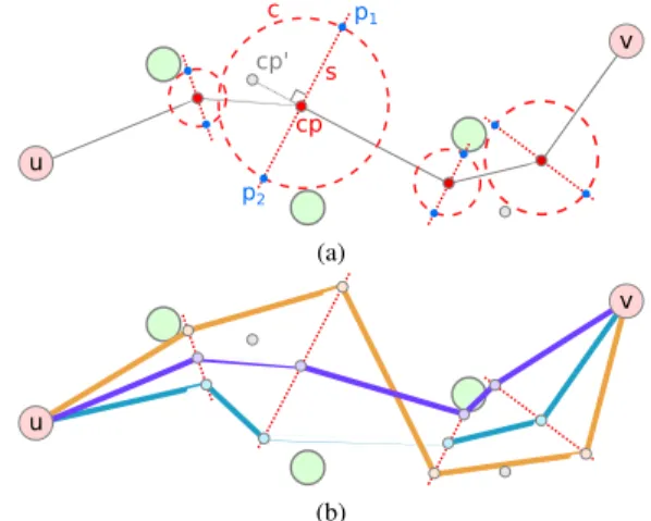
u v c p1 p2 s cp cp' (a) u v (b)
Figure 2: Per Layer Bundle Division: (a) compute the perpen-dicular segment to the control point considering control points that already exist (b) per layer division of control points.
Then, for each control point we determine a segment that pass through it and intersects the circle determining the free space. For instance, in Figure 2a we can observe that the control pointcpis surrounded by the circlec. Consideringcpandc, we draw the seg-mentsthat intersectscat the points p1andp2.sis drawn
perpen-dicular to the segment linkingcpand the gray control points from which it is generated. In the example in Figure 2a, the segments
is perpendicular to the segment [cp,cp0]. Successively, we dupli-cate the control pointcpinto several control points, one for each edge type of the bundle. Finally, we locate the new control points uniformly ons. Once this operation is done, for each original con-trol point of the bundle, we use the new concon-trol points to draw the different edge types without a particular order (see Figure 2b).
ds (a) ds (b) ds (c)
Figure 3: Bundle Crossing Reduction heuristic: a) initial scenario with bundle crossing b) computation of the barycenters of the projections of the control points neighbors onds(barycenters are depicted with a red border) c) new order of the control points onds.
4.2 Avoiding Edge-Node Overlap
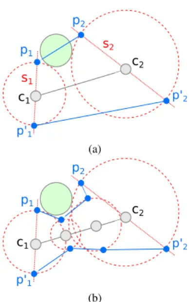
c1 c2 s1 s2 p1 p2 p'1 p'2 (a) c1 c2 p1 p2 p'1 p'2 (b)
Figure 4: Edge-Node overlap heuristic: (a) the issue we can have drawing the per-layer bundles b) the over-discretization heuristic (withK=3) we employ to deal with the edge-node overlap prob-lem.
In a more general scenario, if we consider only the space around the control points to draw the different edge types we can fall in a situation similar to the one reported in Figure 2b (violet segment overlaps green node). As we can observe, one or more of the new segments can overlap the nodes inducing ambiguity in the visu-alization. In order to address this issue, we adopt the following strategy, named Edge-Node overlap heuristic: lets1 (resp. s2) be
the segment incident on control pointc1(resp. c2) as explained in
Section 4.1 and,p1and p01(resp. p2and p02) be the endpoints of
s1 (resp. s2). Then if a nodenfalls into the polygon defined by
the set of points (p1,p2,p02,p01) (see Figure 4a) we over-discretize
the segment[c1,c2]inKsegments addingK−1 control points
uni-formly distributed along its length. Such a trick helps to deal with the overlap issue since new control points are added to refine the bundle division step introduced in Section 4.1 (see Figure 4b). In our approach we fixK=10 as we empirically observe that this number supplies a good trade off between computational complex-ity and visual result.
5 BUNDLE CROSSING REDUCTION
As shown in Figure 3a, the previous steps of our framework can induce edge crossing between edges of different types, affecting the multilayer graph visualization. This phenomenon happens be-cause consecutive control points, traversed by the same type of
edge, could not have the same order on their segment. For instance, we can observe in Figure 3a that control points employed to draw the orange bundle do not have the same relative position along the different segments. To deal with this issue, we adapt the barycenter heuristic, usually employed to draw DAGs [22]. More in detail, in our case we want to find the order of the control points on the line
dsthat minimizes the number of crossing edges. This problem is
closely related to the metro-line crossing minimization task [18]. Alternative heuristics have been proposed in [18] and they could be also adapted to our problem.
Given the lineds and a set of control points lying on it, for a
control point of a particular edge type we compute the barycenter of the projections of its neighbors onds. We repeat the same procedure
for all the control points lying onds. Considering our example
in Figure 3a, Figure 3b shows the barycenter computed for each control point ondsconsidering its neighbors. The barycenters are
highlighted by points ondswith red border. Then, the control points
ofsare reordered according to the computed barycenter obtaining a new order of the original control points as depicted in Figure 3c.
6 CASESTUDIES
In this section we illustrate a case study that shows the practical benefits of our method to visualize multilayer graph data. The case study investigates social interaction among people who com-municate through different media. We employ theReality Mining
dataset1. This multilayer graph contains human interaction data collected by the MIT Media Lab. The experiment was carried out on a total of 94 people and this also represents the number of nodes in the corresponding multilayer graph. The different layers offered by the dataset pertain to the means of interaction between a pair of people. Namely,CALLlayer refers to subjects calling each other, FRIENDlayer contains friendship claims,SMSlayer builds on text message exchanges (SMS) andDEVICElayer contains Bluetooth device scans. For our purpose we consider the first three layers (CALL,FRIENDandSMS) discarding theDEVICElayer as it is a quasi-clique and it does not provide useful information in the con-text of edge bundling visualization. The three considered layers have, respectively, 177, 82 and 113 edges. Experiments are carried out on an Desktop Computer with Intel Core i7-3770 CPU @ 3.40 GHz x 8, with 8 Gb of RAM.
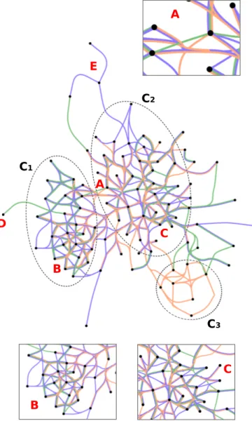
Figure 5 shows the result of our multilayer graph edge bundling on the portion of Reality Miningdataset we consider. The vio-let edges correspond to the CALL layer, the green edges corre-spond to theFRIENDlayer andSMSlayer is depicted in orange. Curved edges that are not parts of bundles are artifacts of the initial bundling algorithm (see Section 2). Computation time is of 2.40 seconds with 2 iterations of the edge smoothing process.
Analyzing the visual result, we can note that the graph have three cluster structures: C1,C2 andC3. We can observe thatC1andC2
contain edges of different types whileC3contains only people that 1http://realitycommons.media.mit.edu/
A
B
C
D
E
C
1C
2C
3B
C
A
Figure 5: Result of the multilayer graph edge bundling approach on theReality Miningdataset with three focus on different interaction patterns our method helps to highlight.
interact each other through SMS (SMSlayer in orange). Another interesting fact to point out is the way in which the different com-munities are linked each other. If we focus on how people from communityC1interact with people of communityC2, we can see
that they use SMS (orange layer) and they call each other (violet layer) without necessarily being friends. There is only a green link between this two communities highlighting a friend relationship that constitutes an isolate case or an abnormal interaction behav-ior betweenC1andC2(see Figure 5, letter (A) ). Considering the
way in which people belonging toC2are linked with people in the
communityC3, we can note that some of them are involved in a
friend relationship (green layer) while others employSMS(orange layer) to interact. What is highlighted by the visualization is that no mobileCALL(violet layer) are performed between community
C2andC3. The visualization also supplies the information that no
interactions between the communitiesC2andC3exist.
The multilayer graph edge bundling technique also helps to high-light behaviors that are specific to a portion of the graph. For in-stance, considering clusterC1, we can note that, at the top of this
community, there is a group of people that are friends (green layer)
and interact each other only throughCALL(violet layer) while a different behavior is depicted at the core ofC1where people that
are friends (green layer) communicate with both mobileCALL (vi-olet layer) andSMS(orange layer) as shown in Figure 5 letter (B). In the same way (Figure 5 letter (C)), the core part ofC2contains
people in a friend relationship (green layer) that communicate sim-ilarly as done by the core of communityC1. A different behavior
is shown by communityC3where people belonging to this cluster
only communicate each other withSMS(orange layer).
The visualization allows also to identify some kind of anomalies in the graph structure and the information about the different layers can help to analyze such anomalies. For instance, considering the left part of the graph (see Figure 5 letter (D)), we can observe that an isolate node is connected to communityC1and this (green) link
underlines that this outlier node is a friend of a people belonging to
C1. Another anomalous behavior is shown in the top of the graph
(Figure 5, letter (E)) where, two nodes, that do not belong to any cluster, communicate with other people only through mobileCALL (violet layer). We can found a similar pattern on the extreme right and at the bottom of the multilayer graph. We can consider these nodes as anomalies showing a similar communication pattern. All of them, to some extent, represent community outliers that interact with other people only through mobileCALL(violet layer).
To the sake of completeness, we also evaluate our multilayer graph edge bundling on a bigger multilayer graph composed by 301 nodes and 3 326 edges (considering all the layers). This multilayer graph is a subsample of theBIOGRIDdataset [2], a protein-protein interactions network where nodes represent proteins and edges rep-resent interactions between proteins. This multilayer graph con-tains 8 layers. Figure 6 shows the visualization of theBIOGRID
multilayer graph before (Figure 6a) and after (Figure 6b) our ap-proach is applied. Computation time is 1037.12 seconds with 1 iteration of the edge smoothing process. Also in this case, we can observe that our proposal firstly helps to better emphasize the global multilayer graph structure and secondly it still allows to minimize the edge cluttering issue especially among edges of different type.
(a) (b)
Figure 6: Visualization of the subsample ofBIOGRIDmultilayer graph: a) the visualization before applying our approach b) the re-sult obtained with the multilayer graph edge bundling strategy.
7 CONCLUSION ANDFUTUREWORK
In this paper, we have presented a novel and intuitive technique to route different types of edges into bundles to visualize multilayer graphs. Our approach reduces edge clutter at both global and per layer level. As future work, we plan to consider the number of edges passing through a bundle to determine its width and manage weighted multilayer graph.
REFERENCES
[1] T. Bl¨asius, S. G. Kobourov, and I. Rutter. Simultaneous embedding of planar graphs. InHandbook of Graph Drawing and Visualization, page 349383. CRC Press, 2013.
[2] F. Bonchi, A. Gionis, F. Gullo, and A. Ukkonen. Distance oracles in edge-labeled graphs. InProceedings of the International Conference on Extending Database Technology (EDBT), pages 547–558, 2014. [3] Q. W. Bouts and B. Speckmann. Clustered edge routing. In
Proceed-ings of the IEEE Pacific Visualization Symposium (PacificVis), pages 55–62, 2015.
[4] T. Crnovrsanin, C. Muelder, R. Faris, D. Felmlee, and K.-L. Ma. Vi-sualization techniques for categorical analysis of social networks with multiple edge sets.Social Networks, 37:56–64, 2014.
[5] W. Cui, H. Zhou, H. Qu, P. C. Wong, and X. Li. Geometry-based edge clustering for graph visualization.IEEE Transactions on Visualization Computer Graphics, 14(6):1277–1284, 2008.
[6] M. D. Domenico, M. A. Porter, and A. Arenas. MuxViz: a tool for multilayer analysis and visualization of networks.Journal of Complex Networks, 3:159–176, 2014.
[7] S. Elzen and J. van Wijk. Multivariate network exploration and presen-tation: From detail to overview via selections and aggregations.IEEE Transactions on Visualization and Computer Graphics, 20(12):2310– 2319, 2014.
[8] O. Ersoy, C. Hurter, F. V. Paulovich, G. Cantareiro, and A. Telea. Skeleton-based edge bundling for graph visualization.IEEE Transac-tions on Visualization Computer Graphic, 17(12):2364–2373, 2011. [9] D. Holten. Hierarchical edge bundles: Visualization of adjacency
re-lations in hierarchical data.IEEE Transactions on Visualization Com-puter Graphics, 12(5):741–748, 2006.
[10] D. Holten and J. J. van Wijk. Force-directed edge bundling for graph visualization.Computer Graphics Forum, 28(3):983–990, 2009. [11] C. Hurter, O. Ersoy, and A. Telea. Graph bundling by kernel density
estimation.Computer Graphics Forum, 31(3):865–874, 2012. [12] A. Kerren, H. Purchase, and M. O. Ward. Information
visualization-towards multivariate network visualization (dagstuhl seminar 13201).
Dagstuhl Reports, 3(5), 2013.
[13] A. Lambert, R. Bourqui, and D. Auber. 3D edge bundling for geo-graphical data visualization. InProceedings of the 14th International Conference on Information Visualisation (IV), pages 329–335, 2010. [14] A. Lambert, R. Bourqui, and D. Auber. Winding roads: Routing edges
into bundles.Computer Graphics Forum, 29(3):853–862, 2010. [15] J. Leskovec, A. Singh, and J. Kleinberg. Patterns of influence in a
rec-ommendation network. InProceedings of the Pacific-Asia Conference on Knowledge Discovery and Data Mining (PAKDD), pages 380–389, 2006.
[16] S.-J. Luo, C.-L. Liu, B.-Y. Chen, and K.-L. Ma. Ambiguity-free edge-bundling for interactive graph visualization. IEEE Transactions on Visualization Computer Graphic, 18(5):810–821, 2012.
[17] A. Meidiana and S.-H. Hong. MultiStory: Visual analytics of dynamic multi-relational networks. InProceedings of the IEEE Pacific Visual-ization Symposium (PacificVis), pages 75–79, 2015.
[18] M. N¨ollenburg. An improved algorithm for the metro-line crossing minimization problem. InProceedings of the Conference on Graph Drawing (GD’09), volume 5849 ofLecture Notes in Computer Sci-ence, pages 381–392. Springer, 2010.
[19] D. Redondo, A. Sallaberry, D. Ienco, F. Zaidi, and P. Poncelet. Layer-centered approach for multigraphs visualization. InProceedings of the 19th International Conference on Information Visualisation (IV), pages 50–55, 2015.
[20] B. Renoust, G. Melanc¸on, and T. Munzner. Detangler: Visual ana-lytics for multiplex networks.Computer Graphics Forum, 34(3):321– 330, 2015.
[21] D. Selassie, B. Heller, and J. Heer. Divided edge bundling for direc-tional network data. IEEE Transactions on Visualization Computer Graphics, 17(12):2354–2363, 2011.
[22] K. Sugiyama, S. Tagawa, and M. Toda. Methods for visual under-standing of hierarchical system structures.IEEE Transactions on Sys-tems, Man, and Cybernetics, 11(2):109–125, 1981.
[23] A. Telea and O. Ersoy. Image-based edge bundles: Simplified
visu-alization of large graphs.Computer Graphics Forum, 29(3):843–852, 2010.
[24] A. Zhang. Protein Interaction Networks: Computational Analysis. Cambridge University Press, 2009.