A survey on handling computationally expensive
multiobjective optimization problems with evolutionary
algorithms
Tinkle Chugh
∗ 1, Karthik Sindhya
1, Jussi Hakanen
1, and Kaisa Miettinen
1 1University of Jyvaskyla, Faculty of Information Technology, P.O. Box 35 (Agora),
FI-40014 University of Jyvaskyla, Finland
Abstract
Evolutionary algorithms are widely used for solving multiobjective optimization problems but are often criticized because of a large number of function evaluations needed. Approxi-mations, especially function approxiApproxi-mations, also referred to as surrogates or metamodels are commonly used in the literature to reduce the computation time. This paper presents a survey of 45 different recent algorithms proposed in the literature between 2008-2016 to handle com-putationally expensive multiobjective optimization problems. Several algorithms are discussed based on what kind of an approximation such as problem, function or fitness approximation they use. Most emphasis is given to function approximation based algorithms. We also compare these algorithms based on different criteria such as metamodelling technique and evolutionary algo-rithm used, type and dimensions of the problem solved, handling constraints, training time and the type of evolution control. Furthermore, we identify and discuss some promising elements and major issues among algorithms in the literature related to using an approximation and numerical settings used. In addition, we discuss selecting an algorithm to solve a given com-putationally expensive mmultiobjective optimization problem based on the dimensions in both objective and decision spaces and the computation budget available.
Keywords: surrogate, metamodel, machine learning, multicriteria optimization, computational cost, response surface approximation, Pareto optimality
1
Introduction
Many engineering problems have multiple objectives to be optimized and these objectives are typi-cally conflicting in nature, i.e. improvement in one objective is possible only by allowing deterioration of at least one of the other objectives. These kinds of problems are known as multiobjective opti-mization problems (MOPs). Because of the conflicting nature, there typically does not exist one optimal solution, but multiple so-called Pareto optimal solutions. The set of all Pareto optimal solutions in the objective space is called a Pareto front. In many problems, explicit formulations of objective or constraint functions are not known and such functions are called black box functions. Usually, problems involving such functions need a long time to be solved e.g. problems involving
computational fluid dynamics simulations utilizing finite element algorithms take substantial time to obtain one solution. These are examples of problems that we refer to as computationally expensive multiobjective optimization problems.
In the last few decades, evolutionary algorithms (EAs) [20, 28] have been widely used for solving MOPs because of their advantages such as obtaining a set of nondominated solutions in one solution process, ability to handle problems with multiple local and nonconvex Pareto fronts, ability to easily deal with different kinds of variables (such as binary, real, integer or mixed) and no assumptions set on convexity and differentiability of objectives and constraints involved. Despite of these advantages, EAs do not guarantee convergence to optimal solutions. Moreover, they are often criticized as they consume many function evaluations which increases the computation time. This concern is particularly relevant when dealing with computationally expensive problems. It is therefore required to adapt EAs in a way that they can be used to obtain solutions in less computation time without too much reduction in the quality of solutions. In this paper, a survey of different algorithms proposed in the literature to handle MOPs with computationally expensive objective functions is presented. For other challenges related to solving MOPs, see [20, 28, 93].
Several algorithms have been proposed reduce the computational cost while solving MOPs using EAs. Different surveys exist in the literature [61, 62, 119, 74] on this topic. One of the popular ap-proaches mentioned in these surveys is the use of approximation, especially, function approximation or metamodelling to handle computationally expensive problems. The potential of metamodelling techniques has been widely studied in the machine learning community [41]. Many algorithms exist in the literature which use a combination of these techniques and evolutionary algorithms.
In [61], different ways of using approximation such as problem, function and fitness approxima-tion were discussed based on their use in the literature. Addiapproxima-tionally, various issues such as how evolutionary algorithms can benefit from these approximations and what kind of approximation to be selected etc. were also discussed. It is to be noted that fitness approximation is also used as evolutionary approximation in the literature [61]. In [119], the main focus was to discuss various algorithms proposed in the literature before the year 2008 based on the classification of [61]. Some real-world applications were also mentioned, where different algorithms had been applied to reduce the computation time. In [62], the main focus was to discuss the recent developments for using function approximation in reducing the computation time. In that survey, different issues such as strategies for managing approximation, selection of individuals to be evaluated using approxima-tion funcapproxima-tions etc. were discussed. In addiapproxima-tion, the author also menapproxima-tioned the potential of using function approximation in dynamic, robust and constrained optimization problems. A taxonomy of metamodel based optimization algorithms was provided in [49]. In [74], several algorithms based on the management of using function approximation (e.g. Kriging, radial basis function etc.) were dis-cussed. In addition, the importance of interactive algorithms with EAs was detailed. Two real-world applications were also mentioned, which were solved by two different algorithms, ParEGO [71] and the algorithm proposed in [98].
In this survey, we extend these surveys and discuss 45 algorithms based on the classification of [61] from the year 2008 to 2016 published in different journals and conference proceedings in English. We also found that most of the algorithms use Kriging when compared to other function approximation techniques and therefore, classify different function approximation based algorithms into Kriging and non-Kriging based algorithms. This survey is also different from other surveys in following ways. 1. Algorithms using function approximation or surrogates are emphasized as they are more widely used. 2. Classification of function approximation based algorithms further into Kriging and non-Kriging based algorithms shows the wide applicability of Kriging. 3. Algorithms are described in reference to a general function approximation framework which will provide the reader an understanding for using any function approximation in EAs. 4. The efficiency of different
algorithms in terms of reducing computational cost or number of function evaluations is empha-sized. 5. Various shortcomings in algorithms are observed and discussed e.g. handling constraints, dimensions (both in decision and objective spaces) of the problem solved, training time etc. 6. Some promising elements are also identified which can be helpful in overcoming the limitations of several issues e.g. efficient management of function approximation technique to handle more than three objectives. 7. Some guidelines are also provided in selecting a particular algorithm based on the characteristic of the problem to be solved, dimensions in both objective and decision spaces and the budget available.
In the rest of this paper, in Section 2, some relevant concepts are described which are frequently used when reducing the computational burden. In Section 3, different algorithms are discussed based on the steps of general approximation framework. In addition, different algorithms are compared based on the type of approximation, evolutionary algorithm, evolution control and characteristics of the optimization problem solved. A brief discussion on various issues and using promising elements related to the use of different algorithms is presented in Section 4. Finally, conclusions are drawn in Section 5 along with future research directions.
2
Basic concepts and terminology
We consider multiobjective optimization problems of the form [93]: minimize{f1(x), . . . , fk(x)}
subject tox∈S (1)
with k(≥2) objective functions fi(x) :S → <. The vector of objective function values is denoted
by f(x) = (f1(x), . . . , fk(x))T. For the simplicity of presentation, we assume that all the objective
functions are to be minimized. If some objective function fi is to be maximized, it is equivalent to
minimize −fi. The (nonempty) feasible regionS is a subset of the decision variable space<n and
consists of decision variable vectors x= (x1, . . . , xn)T that satisfy all the constraints. The image
of the feasible space S in the objective space <k is called the feasible objective set denoted byZ.
The elements of Z are called feasible objective vectors denoted byf(x) or z= (z1, . . . , zk)T, where
zi =fi(x), i= 1, . . . , k, are the objective function values.
As discussed in the introduction, objective functions in a MOP are typically conflicting in nature, and, thus, there is no single well-defined optimal solution but a set of so-called Pareto optimal solutions exists. A decision vector x∗∈S is Pareto optimal if there does not exist another decision vector x ∈S such that fi(x) ≤fi(x∗) for all i=1,. . . ,k andfj(x) < fj(x∗) for at least one index
j. An objective vector is Pareto optimal if the corresponding decision vector is Pareto optimal. A Pareto optimal set consists of all Pareto optimal solutions in the decision space and a Pareto front consists of all Pareto optimal solutions in the objective space. A solution x1 ∈S is said to
dominate another solution x2 ∈S, denoted by x1 x2 iff
i(x1)≤fi(x2) for all i= 1, . . . , k and
fi(x1)< fi(x2) for at least onei∈ {1, . . . , k}.
Ideal and nadir objective vectors represent bounds for objective function values in the Pareto front. Components of an ideal objective vectorz∗∈ <kare determined by minimizing each objective
function individually, that is,z∗i = minimize
x∈S fi(x). A nadir objective vector consists of upper bounds
of objective functions in the Pareto front. It is usually difficult to obtain for problems with more than two objectives. Several ways of approximating it have been proposed in the literature (see e.g. [29, 93]). In what follows, we define concepts relevant to the present survey.
Ametamodelis an approximation of some computationally expensive element in a multiobjective optimization problem. A metamodel replaces the computationally expensive element by an element
which consumes less computation time. There can be different computationally expensive elements while solving a MOP. For example, original functions or constraints, hypervolume etc. A surrogate is often used as a synonym for a metamodel and the process to build a metamodel is known as metamodelling or function approximation. Therefore, what to approximate using a metamodel is an important concern in reducing the computation time. Neural networks [94, 145], radial basis functions [111], support vector regression [7] and Kriging [52] are some examples of commonly used metamodelling techniques.
Anensemble of metamodelsmeans using more than one metamodel to reduce the computation time and usually there are two ways to use an ensemble of metamodels in the literature. In the first one, one metamodel having the highest accuracy among different metamodels is selected to evaluate individuals [127]. In the second one, different metamodels are used to evaluate individuals with a different weight coefficient (ωj) assigned to them. For instance, in [84], the predicted fitness value
from an ensemble ofmmetamodels was defined as:
Fens(x) = m X j=1 ωjFj(x) and m X j=1 ωj = 1, (2)
where Fj(x) is the approximated fitness value of F = Pk
i=1wifi(x) using jth metamodel and
wi, i = 1, . . . , k is the weight vector assigned to each objective function. A weighted sum method
was used in [84], however, other scalarizing methods such as -constraint method, achievement scalarizing function [93] can also be used to convert a multiobjective optimization problem into a single objective optimization problem. Fitness values, Fens(x) is approximated by m metamodels
and ωj is the weight assigned to the fitness value of the jth metamodel. The fitness value of a
metamodel is assigned a larger weight if it is found to be more accurate than other metamodels and the accuracy can be obtained by statistical measurements such as root mean square error [132] etc. Anevolution control ormodel management [64] is a strategy to manage metamodels in an EA. There are two different ways to manage metamodels, fixed and adaptive evolution control. In a fixed evolution control, metamodels are used for a prefixed number of generations and updated afterward with a predefined criterion. On the other hand, in an adaptive evolution control, the frequency of using the metamodel is adjusted according to the accuracy of the metamodel. Therefore, the model management is also concerned with when to update the metamodel.
Infitness inheritance[121, 150], the fitness values of offspring are evaluated using fitness values of the parents. In fitness imitation [70], individuals are grouped into several clusters e.g. using K-means clustering [57] in the decision space and only those individuals are evaluated which represent the clusters (e.g. individuals closest to the centroid of each cluster). The fitness values of other individuals are estimated using the fitness values of the representative individuals.
Next, we discuss the general function approximation framework and describe various algorithms based on the steps of the framework.
3
Approximation based algorithms
In approximation based algorithms, the computationally expensive element of the problem is replaced with an approximation which consumes less computation time. As classified in [61], an approxima-tion can be applied in three ways in multiobjective optimizaapproxima-tion problems: problem, funcapproxima-tion and fitness approximation. In problem approximation, the original problem is replaced with a simplified problem which is faster to solve. In function approximation, an approximation of a computationally expensive function is formed which is faster to evaluate. On the other hand, in fitness approxi-mation, the fitness value referring typically to the function value of an individual is derived from
the fitness values of the existing evaluated individuals in its vicinity. The function approximation is more widely used than other approximations and algorithms applying it are discussed next in Section 3.1. Approaches using problem and fitness approximation are discussed in Section 3.2.
3.1
Function approximation
As said, function approximation is the most commonly used approach among approximation based algorithms and there, an explicit or an implicit approximation of a computationally expensive, function is formed, which is faster to evaluate. In what follows, we refer to the functions of the original, computationally expensive problem as original functions. In the literature, metamodel is often used for all objective functions, therefore all objective functions are assumed as computationally expensive. Neural networks [76, 94, 8, 84], Kriging [71, 59, 109, 83] and polynomial regression [52, 127] are examples of algorithms used for function approximation.
The general steps for using function approximation in an EA can be divided into two stages consisting of ten steps and most of the algorithms discussed in this section follow these steps. In what follows, we present a function approximation framework that captures the core of the EA proposed in the literature utilizing function approximation. Additionally, it is assumed that one type of metamodel is used for all objective and constraint functions involved although it is possible to use different metamodels for different objective functions.
Stage 1
1. Initialize the population either randomly or using a sampling method.
2. Evaluate the individuals of the population using the original functions and add them to an archive.
3. If a prefixed number of generations is completed, go to stage 2.
4. Use EA operators (selection, crossover and mutation) to create a new population and go to step 2.
Stage 2
5. Build or update a metamodel for each computationally expensive objective and constraint func-tion using the individuals from the archive.
6. Use EA operators (selection, crossover and mutation) to create a new population.
7. For each objective and constraint function, evaluate the individuals of the new population either using the metamodel or the original function (fixed or adaptive evolution control strategy). 8. If a stopping criterion is met, select the non-dominated individuals from step 7 as the final
population and stop. Otherwise, continue.
9. Select individuals from step 7 for re-evaluation using the original functions if needed.
10. Add the individuals from step 9 to the archive and go to step 5.
In stage 1, a general evolutionary algorithm works and in stage 2, an EA with a metamodel is used. In step 1, a population is initialized either randomly or using a sampling method such as Latin hypercube sampling [91]. Individuals of the population are evaluated using the original functions and the evaluated individuals are added to an archive in step 2. If a prefixed number of generations
is completed in step 3, stage 1 is terminated and the archive is carried over to stage 2. Otherwise, a new population (offspring population) is generated using EA operators such as selection, crossover and mutation in step 4. A prefixed number of generations is required to obtain an archive of a fixed size. In most of the papers cited in this paper, there is no explicit criterion mentioned for choosing the prefixed number of generations. However, it is mentioned in [6] that the prefixed number of generations depends on the dimensions of the problem (both in objective and decision spaces) and the budget of evaluations with the original functions. For instance, in three popular algorithms known as ParEGO [71], SMS-EGO [109] and MOEA/D-EGO [148], a data set of size 11n-1 was used for training the metamodels. We provide the size of the data set used in different algorithms in Table 1.
After completion of stage 1, a metamodel is created for each computationally expensive objective and constraint function to work with the EA algorithm for evaluating individuals in stage 2. A metamodel is created using the individuals from the archive in step 5. In step 6, an offspring population is generated using EA operators. In step 7, either the metamodel or the original functions are used to evaluate individuals i.e. a fixed or an adaptive evolution control strategy is used to manage the metamodel. In step 8, if a termination criterion such as maximum number of generations or function evaluations is met, nondominated individuals from the last population are selected as the final population. Otherwise, some individuals are selected from step 7 and re-evaluated using the original functions in step 9. There are different criteria mentioned in the literature to select individuals for re-evaluation e.g. selection of nondominated individuals, using expected improvement [67], expected hypervolume improvement [109] etc. These individuals are then added to the archive in step 10 to update or re-train the metamodel. If the size of the archive is prefixed, some individuals (e.g. random or dominated individuals) are eliminated from the archive using a predefined criterion.
3.2
Challenges in using metamodels
Before going into the details of different algorithms, we mention here major challenges when applying function approximation in multiobjective optimization when compared to single objective optimiza-tion. It is not straightforward to use a metamodel with an EA because several challenges exist which affect the performance of the metamodel used. These challenges are also the main differences in several algorithms in using function approximation.
1. Using the metamodel: In case of single objective optimization, often one metamodel is used for the approximation of the objective and constraint function. Using metamodels in multi-objective optimization is not that trivial. For example, one can use different metamodels for different objective functions, one metamodel for all objective functions, different metamodels for one objective function or a single metamodel for scalarized objective functions. The same options may arise for different constraints. In the literature, most of the algorithms use a single metamodel for all objective functions. In addition, there are no guidelines for using different metamodels for different objective functions.
2. How to update the metamodel: Updating the metamodel is an important step both in single objective and multiobjective optimization. In case of single objective optimization, different strategies have been used for updating the metamodel e.g. lower confidence bound [33], prob-ability of improvement [135], expected improvement [120, 67] etc. In case of multiobjective optimization, two goals, convergence and diversity have to be achieved in contrast to single objective optimization. In case of multiobjective optimization, one of the simplest ways is to select the nondominated individuals for re-evaluation [63, 64] using the original functions. Alternatively, a clustering method such as K-means clustering [57] can be applied to cluster
the individuals in the objective space and the representative individuals are re-evaluated using the original functions [45, 65]. The representative individuals can be the individuals closest to each cluster center or the best individuals (with highest fitness values) in each cluster. In-dividuals with low approximation accuracy can also be selected for re-evaluation [13, 39] and this selection may be effective in improving the approximation accuracy of the metamodel. In the literature, criteria for updating the metamodel in single objective optimization are also modified to be used in multiobjective optimization. For instance, expected improvement in [71, 60, 69, 24, 140] and probability of improvement in [24] are used to update the metamodel in multiobjective optimization. In addition, expected hypervolume improvement is used in [38, 37, 124] to select the individuals for re-evaluation so that the metamodel can be updated. It is to be noted that infilling criterion is sometimes used as a synonym for updating criterion in the literature.
3. Training time for the metamodel: Training time is also an issue in case of single objective optimization but when moving to multiobjective optimization, training or updating time be-comes more influential. For example, different metamodels for different objective functions may take a different amount of training data (archive size) which increases the training time when compared to single objective optimization. In the literature, unfortunately, most of the algorithms do not mention the training time for the metamodel. This is due to the reason that the training time of the metamodels is usually assumed to be negligible compared to objective function evaluations. However, it may happen that the training time of the metamodels is substantial and the whole aim of reducing computation time is jeopardized.
In addition to the three challenges above, two challenges exist which are common to both single objective and multiobjective optimization. They can influence the performance of an EA while using metamodels.
1. Choice of the metamodel: In the literature, there is very little guidance about the choice of the metamodel for approximation of computationally expensive functions. A metamodel is either selected randomly or due to its popularity in the area with which the problem is associated. For instance, in [76], radial basis neural network was used as a metamodel for approxima-tion of objective funcapproxima-tions in coastal aquifer management problem and it was menapproxima-tioned that neural networks were popular for groundwater applications. Kriging was used in [59] due to its promising nature for building accurate global approximations.In [101], different metamod-elling techniques were used for different problems i.e. RBF with linear kernel function for ZDT problems and Kriging for UF [149] problems. The reason mentioned was that RBF was used due to simplicity of the function landscape in ZDT problems and and Kriging was used be-cause functions in UF problems are highly non-linear and test with RBF showed a very low accuracy when used for UF problems. However, the algorithm was developed for black-box computationally expensive problems, where function landscape of the problems in question is not known a priori. Moreover, Kriging is most popular technique when compared to others because of its ability to provide uncertainty for the approximated values. To overcome the problem of choosing of a metamodel, an ensemble of metamodels described in Section 2 is also used in the literature [127, 84]. However, there are still some open challenges related to the ensemble of metamodels such as what should be the criterion for choosing different metamodels or how different metamodels can be used simultaneously?
2. When to update the metamodel: It is also an important issue to decide when to update the metamodel or in other words, is there any need to update the metamodel. For example, before selecting individuals in step 9, one can check whether the existing metamodel is accurate
enough to predict objective function values in the next generation. If so, the metamodel is not updated and the existing metamodel is used for approximation. An offspring population has to be generated before updating the metamodel so that the metamodel accuracy can be measured for the individuals of the offspring population. There may be a possibility that the metamodel is never updated and the metamodel trained after stage 1 is used in all generations. In that situation, steps 9 and 10 are eliminated from stage 2. In the literature, there is very little focus on the question of when to update the metamodel.
3. Handling constraints: While using metamodels in constrained problems, an appropriate set of solutions is needed to train them. Most of the metamodel-based algorithms in the literature are not developed to handle constraints. In addition, few algorithms which are developed to handle constraints assume that feasible solutions are available to train metamodels for constraint function. In many problem, obtaining a feasible solution is not trivial e.g. C1-DTLZ1 problem [58] with very small feasible region. In such instances, using metamodels for constraints can be very challenging. We provide more details of handling constraints while describing different algorithms.
Steps 5, 9 and 10 representing the first three main challenges are written in italics in the function approximation framework to indicate the steps, where algorithms using function approximation in multiobjective optimization mainly differ from each other. Other three challenges, selection of a metamodel, when to update the metamodel and size of the data to train the metamodel are not the major differences in the algorithms.
In what follows, 30 algorithms and from the literature are discussed utilizing the three main steps (5,9 and 10) of the function approximation framework and attention is paid to their efficiency in reducing the computation time. These algorithms are classified according to the number of metamodels they have used e.g. single metamodel, multiple metamodels independently or ensemble of metamodels. Among single metamodel based algorithms, Kriging is used more often than other metamodels. As mentioned, the main advantage from Kriging is the uncertainty information besides the predicted objective and/or constraint function values. This uncertainty information can be further utilized in the algorithm. For instance, uncertainty information is used while updating the metamodel in [37, 18, 110, 71].
In contrast to single metamodel based algorithms, some algorithms use metamodels indepen-dently. Moreover, some algorithms use ensemble of metamodels to solve the problem of choosing a metamodel. In what follows, three categories, algorithms based on single metamodel, algorithms based on multiple metamodels and algorithms based on ensemble of metamodels, are used to de-scribe different algorithms. It was found that the number of papers in the literature belonging to the function approximation are largely skewed towards the first category, i.e. algorithms based on a single metamodel. Hence a sub-classification based on the usage of metamodel within different algorithms is devised to enhance clarity and readability. Thus we further classify the algorithms using single metamodel into Kriging and non-Kriging based algorithm. Due to a limited number of articles in other categories, such a sub-classification is not used for others. It is also worth mention-ing that most of the algorithms are based on dominance based EAs and are generic for usmention-ing any metamodel. At the end of this section, a comparison is presented based on which metamodel and type of EAs are used, what is the evolution control strategy and what are the characteristics of the optimization problems.
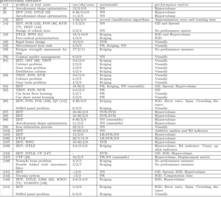
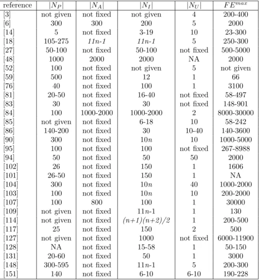
Parameter values used in these algorithms in stages 1 and 2 of the function approximation framework are presented in Table 1, where “NA” indicates that the parameter is not applicable to the algorithm and “not given” means that this information is not given in the reference. The table collects information of the population size in step 1, the size of archive in step 2, the prefixed number
of generations in step 3 in stage 1 and the number of individuals for re-evaluation in step 9 in stage 2, as reported for example problems solved in the papers cited.
All parameters mentioned in Table 1 are important and can influence the performance of the algorithm. The population size|NP|is a critical parameter and several studies like [16, 22] show the
effect of the population size on the performance of evolutionary algorithms. The size of the archive
|NA|mainly affects the training time of the metamodels and as can be seen from the table, most of
the algorithm do not have a fixed size archive. The size of data set|NI|used to train metamodels is
different in different algorithms. One can adjust this parameter based on the resources or maximum number of function evaluations available. In addition, the size of the data set |NU| to update the
surrogates is also important and should be decided based on the resources available. For instance, if it is possible to do parallel evaluations, one can select the size accordingly. An example is given in [72], where the ParEGO algorithm could not be applied in doing experiments for drug design because the algorithm did not have an option to select multiple sample points at a time. The maximum number of function evaluations F Emax is also important when comparing different algorithms.
Many algorithms use different numbers of function evaluations, which makes it difficult to select an algorithm to solve a given problem. The number varies from 50 to 30000 in the literature. Next, we classify algorithms which use only a single metamodel, which are further classified into Kriging and non-Kriging based algorithms.
3.3
Algorithms based on a single metamodel
In this subsection, we discuss algorithms using one metamodel for all objective and/or constraint function. As mentioned, to make the a clear structure of the paper and also due to wide applicability of Kriging models, we further classify this subsection into Kriging based algorithms and non-Kriging based algorithms. Further these algorithms are discussed year wise, i.e. starting from the year 2008.
3.3.1 Kriging based algorithms
In this section, we discuss algorithms using Kriging.
A DACE model [118] which is a Kriging based approximation was used in [109]. This algorithm is known as SMS-EGO which is an extension of efficient global optimization (EGO) [67] for multi-objective optimization problems. In step 5, the metamodel is built for each multi-objective function and to update it in step 9, one individual having maximum contribution to the hypervolume is selected for re-evaluation using the original functions. This individual is then added to the archive in step 10 and the metamodel is updated in the next generation. The size of the archive is not fixed in this algorithm.
SMS-EGO was tested on five benchmark problems (2-5 objectives and 3-6 decision variables) and compared with ParEGO [71] and the algorithm proposed in [60]. The unary hypervolume indicator [156], the R2 indicator [46] and the unary epsilon indicator [157] were used as the comparison criteria. The proposed algorithm performed better than the other algorithms in all cases when hypervolume was used as the performance measure. In terms of other comparison criteria, it performed worse than the other algorithms for three problems.
In Li et al. [83], Kriging was used as a metamodel with a modified version of NSGA-II. In this algorithm which is known as K-MOGA, the metamodel is used for approximating each objective function in step 5. To update the metamodel in step 9, domination status is measured for each individual evaluated using the metamodel. Individuals which change the domination status are re-evaluated using the original functions and added to the archive in step 10. To check the domination status, minimum of minimum distance (MMD) is measured. To calculate MMD, individuals are
Table 1: Parameter values used in different algorithms: |NP|= population size in EA,|NA|= size of
archive in step 10, |NI|= size of the data set to train metamodels in step 5,|NU|= size of the data
set for updating the metamodels and maximum
reference |NP| |NA| |NI| |NU| F Emax
[3] not given not fixed not given 4 200-400
[6] 300 300 200 5 2000
[14] 5 not fixed 3-19 10 23-300
[18] 105-275 11n-1 11n-1 5 250-300
[27] 50-100 not fixed 50-100 not fixed 500-5000
[48] 1000 2000 2000 NA 2000
[52] 100 not fixed not given 5 not given
[59] 500 not fixed 12 1 66
[76] 40 not fixed 100 1 3100
[81] 20-50 not fixed 16-40 not fixed 58-497
[83] 30 not fixed 30 not fixed 148-901
[84] 100 1000-2000 1000-2000 2 8000-30000
[85] not given not fixed 6-18 10 58-242
[86] 140-200 not fixed 30 10-40 140-3600
[90] 300 not fixed 10n 10 1000-5000
[95] 100 not fixed 100 not fixed 267-8988
[94] 50 not fixed 50 50 2000 [102] 26 not fixed 150 1 1606 [101] 26-50 not fixed 150 1 NA [104] 300 not fixed 10n 40 1000-2000 [103] 100 not fixed 10n 10 200-2000 [107] 100 800 100 1 30000
[109] not given not fixed 11n-1 1 130
[114] not given not fixed (n+1)(n+2)/2 1 200-500
[117] 25 not fixed 150 2 500
[127] not given not fixed 1000 not fixed 6000-11900
[128] NA not fixed 15-58 1 50-150
[131] 20-60 not fixed 50 1 3000
[148] 300-595 not fixed 11n-1 5 200-300
partitioned into two sets in the decision space, nondominated (xnd) and dominated (xd). MMD is
calculated as, MMD = minn ˆ f(xnd)−fˆ(xd) o
, where ˆf is the predicted objective vector using the metamodel. MMD is then projected to each objective function axis to obtain MMD ˆfi (for i
= 1,. . .,k). Thereafter, a threshold si(x) ≤ MMD ˆfi is specified by using the standard deviation
obtained (si(x)) from the Kriging model for each objective function. The individuals which do not
satisfy this threshold are re-evaluated using the original functions. The size of the archive is not fixed in this algorithm.
K-MOGA was tested on five benchmark (two objectives and 3-6 decision variables) and two real-world problems (two objectives and 2-4 decision variables) and compared with MOGA. For comparison, nondominated individuals from both algorithms were visualized and similar solutions were obtained in fewer function evaluations with K-MOGA.
The same algorithm was extended to MOGA in [81] with one additional element. In KD-MOGA, a fixed number of individuals is generated using constrained maximum entropy design after step 9, which is an extension of unconstrained maximum entropy design [25]. These individuals are then added to the population for the next generation.
KD-MOGA was tested on the same set of problems as K-MOGA with one more real-world prob-lem (two objectives, four decision variables and four constraints). It was compared with both EAs (modified version of NSGA-II) and K-MOGA using visualization of the nondominated individuals. A similar performance was obtained in fewer function evaluations with KD-MOGA.
Kriging was used as a metamodel in [59]. This paper is based on an algorithm called combined AASO-AAMO (adaptive approximation in single objective optimization - adaptive approximation in multiobjective optimization) [144] which uses a multiobjective genetic algorithm [144] as an EA. The metamodel is built for each objective and constraint function in step 5. To update the metamodel in step 9, a fixed number of individuals is selected for re-evaluation using the original functions and added to the archive in step 10. The individuals having the best value according to the maxmin distance design criterion [66], i.e. the largest value of minimum distance from individuals in the archive in the decision space, are selected for re-evaluation. The size of the archive is not fixed in this algorithm.
The proposed algorithm was tested on a fatigue design MOP with two objectives, 17 decision variables and 11 constraints. It took 70 hours to complete 25 generations but the efficiency of the algorithm was not compared to any EA without using the metamodel. The authors mentioned that it was practically impossible to do the optimization without using approximation.
In Zhang et al. [148], Kriging was used as a metamodel with the decomposition based EA MOEA/D [146]. The algorithm is known as MOEA/D-EGO. In MOEA/D-EGO, after evaluating a fixed number of individuals in steps 1-4, the metamodel is built for the scalarized objective func-tion. Chebyshev scalarizing function [93] is used to convert multiobjective optimization problem into single objective optimization problems. After using the metamodel in step 7, the expected im-provement (EI) [67] is calculated for each subproblem. Expected improvement is then maximized (for each subproblem) using MOEA/D-DE [82] for a fixed number of generations. In other words, the scalarized problem is changed into another problem to maximizeEI. To update the metamodel in step 9, firstly, all individuals after the local search, which are different from the individuals in the archive (in the decision space) are selected. After this, K-means clustering is used to cluster the weight vectors (used in MOEA/D initially) associated with the individuals selected above. From each cluster, an individual with maximum EI is selected and re-evaluated using the original functions. These individuals are then added to the archive in step 10. Moreover, to reduce the training time, a fuzzy clustering [12] is used for selecting a fixed number of individuals for training or updating the metamodel.
MOEA/D-EGO was tested on 12 benchmark problems (2-3 objectives and 2-8 decision variables) and compared with ParEGO [71] and SMS-EGO [110]. Hypervolume and inverted generational distance (IGD) were used as the comparison criteria. The proposed algorithm outperformed on seven problems when compared to ParEGO and performed similar to SMS-EGO. It was also compared with MOEA/D on two problems (two objectives and 2-8 decision variables) and outperformed with IGD as the performance criterion.
A multiobjective variable-fidelity optimization (VFO) algorithm was proposed in [151], where Kriging was used as a metamodel with NSGA-II. Initially, a simplified or approximated problem (having low fidelity functions) is used to replace the original MOP in stage 1. This simplified problem is then solved for a prefixed number of generations using NSGA-II. A fixed number of nondominated individuals obtained after this step is re-evaluated using the original functions and stored in an archive. These individuals are selected based on a simple inter-individual distance metric in the objective space (steps 1-4). These individuals are then used to construct a Kriging model for each objective function in step 5 of stage 2. For the following fixed number of generations, individuals generated by crossover and mutation in step 6 are evaluated either using the approximated problem functions with Kriging model or just the approximated problem functions (step 7) depending on the error [42] in the Kriging model. Thus, an adaptive evolution control strategy is used to manage the metamodel. In other words, if the metamodel is not accurate for an objective function, the original function is used to evaluate individuals. To update the metamodel in step 9, a fixed number of nondominated individuals evaluated using the metamodel is selected for re-evaluation using the original functions. The individuals are selected by computing the error from the Kriging model and added to the archive in step 10. The size of the archive is not fixed in this algorithm.
The VFO algorithm was tested on the ZDT1-3 benchmark problems (with two objectives and five decision variables) and a structural engineering problem (with two objectives and six decision variables). For the ZDT problems, the efficiency of the VFO algorithm was not mentioned in terms of computation time or number of function evaluations.
For the structural engineering problem, an exhaustive search was carried out with different values of decision variables. Around 65 million combinations of decision variable values were evaluated using both original and approximated problem functions. Nondominated individuals after this search were identified and nondominated individuals obtained using original functions were used to compare results of different studies mentioned next. Fourteen studies were performed with changes in the values of three parameters: number of prefixed number of generations in step 3 of stage 1, number of generations before updating the metamodel of stage 2 and number of individuals selected for re-evaluation in step 9 of stage 2. Two out of fourteen studies were performed using NSGA-II without using a metamodel with high and low fidelity functions (to be called case 1 and case 2, respectively). Results from these studies were then compared with the results of exhaustive search with different criteria (inverted generational distance, error ratio, crowding distance [28] and span [80]). Case 1 gave the best results and in comparison with case 1, one of the studies out of thirteen gave similar results (a graphical comparison was performed) in fewer function evaluations.
In [86], VFO algorithm was extended, where instead of one global metamodel, multiple local metamodels were used. The authors mentioned that local metamodels are used for high dimensional problems in the objective space. K-means clustering is used in the decision space to partition the data and to build multiple local metamodels. Other details are the same as in VFO.
This algorithm was tested on six benchmark problems (two objectives and 2-30 decision variables) and one real-world problem (three objectives and six decision variables). For benchmark problem, nondominated individuals obtained from this algorithm and with VFO and NSGA-II were visualized. The authors mentioned that the proposed algorithm outperformed on these problems. In case of the real-world problem, the same performance criterion was used as in the VFO algorithm. In this
case too, the proposed algorithm performed better than NSGA-II and VFO in the same number of function evaluations.
In [128], Kriging was used as a metamodel. In this algorithm, the main focus was to apply different strategy for objective and constraint functions while updating the metamodel. In step 5, a metamodel is built for each objective and constraint function. To update the metamodel in step 9, for objectives, selection is performed using hypervolume based probability of improvement (P OIhv)
[24] and for constraints, probability of feasibility (POF) [41] is used. After this,γ=P OIhv×P OF
is obtained and a fixed number of individuals with highest γ values is selected for re-evaluation in step 9. These individuals are then added to the archive in step 10. The size of the archive is not fixed in this algorithm.
The proposed algorithm was tested on two real-world problems with two objectives, 2-3 decision variables and 5-7 constraints. This algorithm was implemented using the SUrrogate MOdeling MATLAB Toolbox (SUMO) [44] and was not compared with any other algorithm.
In [95], Kriging models were used with a differential evolution based EA to approximate the objective functions. After building the metamodels in step 5, individuals were generated using differential evolution operator in step 6 and metamodels were then used for approximation in step 7. For each offspring in step 7, uncertainties of the approximated values were compared to its corresponding parent. In other words, if the uncertainty value of offspring was less than that of parent, it would selected and kept in the population. On the other hand, if the uncertainties of both offspring and parent are comparable, both are kept in the population. All the offspring thus selected were re-evaluated with the original function to update the metamodels in step 9 and added the training archive in step 10.
The algorithm was tested on 12 benchmark problem out of which three had constraints. However, it was not mentioned in the article how the constraints were handled. All these 12 problems had two objectives and the number of decision variables for all problems was not mentioned. The algorithm was also tested on a continuous steel casting and an electrocardiography problem with four variables and 2-3 objectives. The algorithm was compared with differential based EA [116] and an algorithm based on NSGA-II-ANN [30]. The algorithm obtained better performance when measured with hypervolume in 10000 function evaluations.
In Chugh et al. [18], an algorithm called K-RVEA was proposed to solve computationally ex-pensive problems with more than three objectives. In this algorithm, the metamodels were updated based on the need of convergence or diversity. Angle penalized distance [17] and uncertainty infor-mation from the Kriging models with the help of reference vectors are used to select individuals in step 9 for updating the metamodels. In addition, extra individuals are removed from the archive in step 10 to further reduce the computation time.
The proposed algorithm was tested on DTLZ and WFG benchmark problems with 3-10 objectives and 10 decision variables. It was also compared with ParEGO, MOEA/D-EGO and SMS-EGO using IGD and hypervolume. In addition to benchmark problems, the algorithm was also tested on a free-radical polymerization problem [96] and also compared with the state-of-the-art algorithms. In the given number of function evaluations, the proposed algorithm performed better than other algorithms.
The same algorithm was also extended to handle constraints in [19]. Three different approaches are used to while training metamodels based on the feasibility of solutions. The proposed algorithm was tested on constrained version of DTLZ problems [58] with 3-10 objectives and 10 decision variables. The authors found out that infeasible solutions are having a vital role on the performance of surrogates.
In Roy and Deb [117], a high dimensional model representation (HDMR) [130] was used as a metamodel for each objective function. Kriging was further used within HDMR to approximate
its component functions. The algorithm was proposed to handle problems with large number of decision variables. In each HDMR model,n component functions were approximated using Kriging, therefore n×k (n and k represent the number of decision variables and objectives respectively) Kriging models were built and k HDMR models were built. After building the metamodels in step 5, NSGA-II was used to from steps 6-7. To update HDMR models, a prefixed number of individuals were re-evaluated using the original functions in step 9. These individuals were selected by doing clustering in the decision space and then added to the training archive in step 10. In addition, bounds of the decision variables were updated to limit the search space after metamodels were updated.
The algorithm was tested on 17 benchmark problems from ZDT, DTLZ and CEC09 suite [149] biobjective problems with 15-30 decision variables. It was compared with NSGA-II and Kriging based NSGA-II [89] using IGD and performed better than others in 500 function evaluations.
3.3.2 Non-Kriging based algorithms
In this subsection, algorithms using metamodels other than Kriging such as neural network, support vector regression and polynomial regression are discussed.
In [131], a multiobjective parallel surrogate-assisted evolutionary algorithm (MOPSA-EA) was proposed, where a feedforward neural network was used as a metamodel with a steady state EA. The metamodel is built for each objective function in step 5. A fixed number of offspring individuals is generated in step 6 using crossover and mutation and evaluated using the metamodel in step 7. The fitness values of offspring individuals are altered as per the fitness values of parents. The authors mentioned that this approach was motivated by fitness inheritance, where the fitness values of offspring depend on the fitness values of parents.
To get the altered fitness values for offspring individuals, the parents which are used for creating the offspring individual are evaluated with the metamodel and the error is calculated between true fitness values and the approximated fitness values (using the metamodel) for parents. For example, if the errors (for a biobjective optimization problem) between the true fitness values and the approx-imated fitness values for two parents are (ae, be) and (ce, de) and an offspring individual is generated
using these parents having fitness values (e, g), then the new altered fitness values for offspring are (e+w1×ae+w2×ce, g+w2×be+w1×de). The weight coefficientsw1 andw2 are selected based
on the influence of parent individuals on an offspring individual during crossover. An individual is selected in step 9 after getting new fitness values for offspring individuals and added to the archive in step 10 to update the metamodel. To select this individual, a nondominated sorting for offspring individuals and individuals in the archive is performed and nondominated individuals in both sets are identified. Let OR1 and PR1 denote nondominated individuals in offspring and in the archive,
respectively. These individuals are combined and individuals in OR1 dominatingPR1are identified.
Among these individuals, individual having the largest Euclidean distance to its closest individual in
PR1is selected and added to the archive. A nondominated sorting is performed again for individuals
of the archive and the worst individual (having the worst fitness value and the smallest crowding distance) is removed from the archive. The size of the archive is fixed in this algorithm.
The MOPSA-EA was tested on the ZDT1-4 and ZDT6 benchmark problems (2 objectives and not explicit information of the number of decision variables) and on a manufacturing MOP (with two objectives and 11 decision variables). Generational distance (GD), inverted generational distance (IGD), spread and hypervolume metrics were used to compare the proposed algorithm with SMS-EMOA [36], MAES [38] and NSGA-II-ANN [97]. For the same number of function evaluations, MOPSA-EA performed better than other algorithms inY, Ω andS metrics and in ∆, SMS-EMOA and MOPSA-EA performed equivalent. As the Pareto front was not known for the manufacturing problem, only the S metric was used as the performance criterion and MOPSA-EA gave better
results inS than the other algorithms in the same number of function evaluations.
A quadratic polynomial approximation was used as a metamodel with the EAµ-MOGA [21] in Liu et al. [85]. In this algorithm, the bounds of decision variables are updated after every generation using a trust region algorithm. In step 5, the metamodel is built for each objective and constraint function. To update the metamodel in step 9, a fixed number of uniformly distributed individuals (Pa) from nondominated individuals is re-evaluated using the original functions. The nondominated
individuals in the decision space after re-evaluation are stored in a set Pe. The set Po =Pa ∩Pe
is determined which is then used to calculate a reliability index N(Po)/N(Pa), where N(Po) and
N(Pa) are the numbers of individuals inPoand the number of nondominated uniformly distributed
individuals evaluated using the metamodel, respectively. This reliability index is used to update the bounds of the decision variables in the next generation with a trust region algorithm. The trust region radius is updated according to [4] and the algorithm terminates if the trust region radius is smaller than a predefined limit or after a fixed number of generations (step 8). A Latin hypercube design is used for sampling the decision variables with updated bounds. These individuals with the updated bounds are evaluated with the original functions which are used to update the metamodel. Step 10 is not applicable in this algorithm as individuals after step 9 are not added to the archive.
The proposed algorithm was compared withµ-MOGA using two benchmark problems (two ob-jectives and 2-3 decision variables) and one structural engineering problem (two obob-jectives, three decision variables and one constraint). Using generational distance as a performance metric for the benchmark problems and visual comparison for the structural engineering problem the quality of the obtained set of nondominated solutions within a fixed budget of function evaluations usingµ-MOGA with metamodel was better.
A feedforward neural network was used as a metamodel with NSGA-II in [94]. The metamodel is built for each objective function in step 5 if a threshold based on a predicted tolerance is satisfied. This predicted tolerance, which is an indication of the accuracy of the metamodel, is calculated (however, calculation of the predicted tolerance is not detailed in the paper) after every generation. If this predicted tolerance is less than a user-specified tolerance, then the metamodel is used in the next generation. Otherwise, the original functions are used to evaluate individuals. The predicted tolerance is updated after every generation and again a decision is to be made either to use the original functions or the metamodel and thus, an adaptive evolution control strategy is used. Indi-viduals obtained after every generation are added to the archive (steps 9 and 10) and as a result, the size of the archive grows with generations. In this algorithm, the metamodel is not updated after every generation but after every generation, it is checked whether the existing metamodel is sufficient enough to predict function values to the extent of accuracy required.
This algorithm was tested on an iron induration MOP with two objectives, 22 decision variables and three constraints. To check the efficiency of the proposed algorithm, a graphical comparison was presented to the solutions from the algorithm and NSGA-II without using any metamodel. Similar nondominated individuals were obtained in 50% fewer function evaluations and for the same number of function evaluations, better nondominated individuals were obtained.
In Chen et al. [14], an extension of algorithm proposed in [85] was proposed. The main differences include the type of metamodel, stopping criterion in step 8 and selection of individuals for re-evaluation for updating the metamodel in step 9. The algorithm proposed utilizes a radial basis function as a metamodel. In addition to the stopping criteria posed in [85] mentioned earlier, the algorithm also terminates if the bounds of the decision variables are equal to predefined limit and the reliability index is equal to one. In step 9, the individuals are selected using an inherited Latin hypercube design (ILHD) [141] and a local-densifying strategy (to reduce the possibility of an ill-conditioned RBF matrix) for re-evaluation and subsequently updating the RBF.
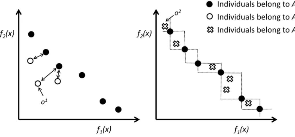
f1(x) f2(x) f1(x) f2(x) Individuals belong to A Individuals belong to A1 Individuals belong to A2 o1 o2
Figure 1: Selection of individual from individuals evaluated using metamodel
decision variables) and a structural engineering problem (two objectives and five decision variables). The results were compared with µ-MOGA without any metamodel and the algorithm proposed in [85]. In case of benchmark problems, the proposed algorithm obtained better values for spread and convergence metrices [31] in fewer function evaluations. For the structural engineering problem, the proposed algorithm was not tested using µ-MOGA without any metamodel.
In [76], a multiobjective surrogate assisted (MOSA) algorithm was proposed, where a modular neural network (MNN) [75] was used as a metamodel with NSGA-II. A metamodel is built for each objective function in step 5. A fixed number (equal to the population size of NSGA-II) of better performing individuals (the authors did not mention any criterion for defining better performing individuals) is used as the population of NSGA-II and the nondominated individuals (A) after this step are determined. The nondominated individuals after evaluating the offspring individuals (generated in step 6) are compared withAto select one individual for re-evaluation (step 9). To do this, the individuals evaluated using the metamodel are clustered into two setsA1 andA2as shown
in Figure 1. The first set (A1) consists of the individuals which dominate at least one individual
ofA while the second set (A2) consists of the individuals that do not dominate nor are dominated.
For each offspring inA1, the Euclidean distances between the offspring and the individuals inAare
calculated. As shown in left part of Figure 1, individual (o1) with the largest distance is selected for
re-evaluation using the original functions. In caseA1is empty, an individual is selected from the set
A2 for re-evaluation. To select the individual, for each offspring individual in A2, the normalized
perimeter for rectangles created between consecutive individuals in A (as shown in the right part of Figure 1) is calculated. An individual located in the rectangle with the largest perimeter (o2) is
selected for re-evaluation using the original functions. In case both A1 andA2 are empty, offspring are generated again. However, the authors did not mention about how this algorithm can be used for more than two objectives. The selected individual is added to the archive to update the metamodel in step 10. The size of the archive is not fixed in this algorithm.
The algorithm was used to solve a coastal aquifer management optimization problem with two objectives and eight decision variables. The time required to evaluate the original functions was 26 hours while the time to train the metamodels was 63 minutes. A graphical comparison was presented between MOSA and NSGA-II and the proposed algorithm gave similar results in fewer function evaluations.
In Herrera et al. [48], support vector regression was used as a metamodel for approximation of each objective function with NSGA-II. The main focus in this algorithm is to use different basis functions for different kinds of variables such as discrete, continuous and categorical variables. It is to be noted that this algorithm does not use an ensemble of metamodels as only one prediction is obtained for each objective function by using different basis functions for the different kinds of variables. To convert categorical values into real number, dummy coding is used. In step 5, the metamodel is built for each objective function. Steps 9 and 10 are not applicable to this algorithm as the metamodel and the archive are not updated.
The proposed algorithm was tested on one real-world problem (two objectives and 10 decision variables) and compared with NSGA-II. Out of 10 variables, 5 were continuous and 5 were categorical variables. A visualization of nondominated individuals in the objective space was performed to compare the two algorithms. The authors mentioned that the proposed algorithm performed similar to NSGA-II in fewer function evaluations.
In [107], support vector regression was used as a metamodel. This algorithm is known as HO-MOMA, where a metamodel is built for each objective function in step 5. After evaluating new individuals in step 7, a local search is used to optimize the fitness function obtained from the metamodel evaluations. This is done as follows. Firstly, several nondominated fronts are obtained with nondominated sorting. Then, in each front, sorting is performed according to the first objective function values in the ascending order. A reference point is then calculated for each individual in each front using these sorted values. After calculating the reference point, a fitness value for each individual is calculated. Let ˆf =nfˆ1,fˆ2
o
be the predicted objective vector for one individual and
r={r1, r2}the reference point for that individual. Fitness is then calculated as
fitness = (r1−fˆ1)(r2−fˆ2) fˆ1< r1 and ˆf2< r2= 0 (r1−fˆ1) fˆ1> r1 and ˆf2< r2= 0 (r2−fˆ2) fˆ1< r1 and ˆf2> r2= 0 −d(r,fˆ) otherwise, (3)
whered(r,fˆ) is the Euclidean distance betweenrand ˆf. This fitness is then optimized using CMA-ES [47] as the local search algorithm. To update the metamodel in step 9, nondominated individuals obtained after the local search are added to the archive in step 10. The size of the archive is fixed in this algorithm and extra individuals are removed from it randomly. The authors mention the study for more than two objectives is a future research.
HO-MOMA was tested on 14 benchmark problems with two objectives and 10-30 decision vari-ables. The algorithm was compared with NSGA-II and ASM-MOMA [105] with hypervolume as the performance criterion. The proposed algorithm performed better than the others in nine out of 12 problems.
In [104, 103], an extreme learning based MOEA/D-DE [82] was used. This algorithm is known as ELMOEA/D-DE and inspired by MOEA/D-RBF. The main focus in this algorithm is to use the metamodel for higher dimensional problems in the decision space. Extreme learning is a single-layer feedforward neural network proposed in [50]. In step 5, the metamodel is built for each objective function. To update the metamodel in step 9, the same procedure is used as in MOEA/D-RBF. In addition, a minimum distance (in the decision space) is maintained between the individuals to be selected for re-evaluation. After adding these individuals in the archive, inferior solutions (in terms of scalarized single objective problem) are removed. Otherwise, the closest individual in the objective space is replaced by the individual obtained in step 9. This is done to ensure that every new solution is added to the archive for updating the metamodel.
ELMOEA/D-DE in [104] was tested on ZDT problems with 10-60 decision variables and com-pared with MOEA/D-DE and MOEA/D-RBF.Later in [103], the algorithm was tested on ZDT, DTLZ and WFG problems with 2-5 objectives and 5-60 decision variables and on an airfoil shape optimization problem with two objectives and 12 decision variables. The algorithm was also com-pared using addictive-Epsilon andR2[156] as the performance indicators. For the given number of
function evaluations, the proposed algorithm obtained better performance.
In [3], an algorithm called gap optimized multiobjective optimization using response surfaces (GOMORS) was proposed, where radial basis functions were used to approximate the objective functions. After building the metamodels in step 5 for each objective function, an EA proposed in [139] was used for optimization from step 6-7. After step 7, an another optimization problem was solved using the same EA by reducing the bounds of the decision variables. This problem was referred as gap optimization problem in the article. In step 9 for updating the metamodels, four criterion were used and one individual corresponding to these criterion was selected and added to the training archive in step 10. Four criterion were based on hypervolume, distance to the individuals in the decision space, distance to the individuals in the objective space and hypervolume in the gap optimization problem. A maximum number of function evaluations was used as the termination criterion.
The algorithm was tested on 11 benchmark problems with 8-24 decision variables and two ob-jectives. In addition, a groundwater remediation problem with 6-24 variables and two objectives was also solved. The algorithm was compared with NSGA-II and ParEGO using hypervolume in 200-400 function evaluations. The proposed algorithms obtained better performance than others in the given number of function evaluations.
In [102], an algorithm called surrogate assisted local search memetic algorithm (SS-MOMA) was proposed, where RBF as a metamodel was build on the single objective problem after converting multiobjective optimization problem using a scalarization function. Two common ways of scalar-ization i.e. Tchebycheff and weighted sum were tested, where weights were generated randomly and the reference point in Tchebycheff scalarization was the current individual objective function val-ues. After generating the offspring population in step 6, metamodels were built locally for each individual. For instance, if the offspring population of size 100 was generated, one metamodel for each individual (i.e. 100 in total) was built. As multiobjective optimization problem was converted into single objective using the scalarzing function, SQP algorithm was used to obtain the solutions. All solutions thus obtained were re-evaluated with the original functions and added to the training archive. Afterward, these solutions were combined with the parent individuals and non-dominated sorting [31] was performed to obtain the population for the next generation. In this way, after every generation metamodels were updated with a number equal to the population size used.
The algorithm was tested on three benchmark problems with 15 variables and two objectives. The algorithm was not compared with any other algorithm. However, in 1606 function evaluations, Tchebycheff scalarization performed better than weighted sum in terms of generational distance [28] and one diversity metric used.
In Datta and Regis [27], RBF as metamodels were built for every objective and constraint function in step 5. A (µ+λ) evolution strategy mutation operator was used to generate new individuals in step 6 which were then evaluated using the metamodels in step 7. After using metamodels for each objective and constraint functions, feasible solutions were found and a nondominated sorting was performed on these feasible solutions. The best individuals i.e. individuals in the first front were re-evaluated with the original functions to update the metamodels in step 9 and added to the training archive in step 10. Therefore, the maximum number of individuals to be updated wasλ. In addition, initial training of metamodels in step 5was performed without considering any feasibility or infeasibility of solutions. However, the authors clearly mentioned that the algorithm is not expected
to work well on problems when the feasible region is empty.
The algorithm was tested on 15 benchmark problems with 2-15 decision variables, 2-5 objective functions and 2-13 constraint functions. In addition it was also tested on a manufacturing and robotics problem with 3-7 decision variables, 2-5 objectives and 2-8 constraints. Hypervolume was used to compare the performance of the algorithm against constrained version of (µ+λ) evolution strategy [9] and NSGA-II. The algorithm performed better in 500-5000 function evaluations.
In [114], RBF was used as a metamodel for each objective and constraint function. It was assumed that at least one feasible solution is available to train the metamodels in step 5. To create new individuals in step 6, two different approaches were tested. In the first one, uniform random individuals were generated over the search space and in the second one, individuals were generated by adding Gaussian perturbation centered at the nondominated individual that has the most isolated objective function values. The most isolated individuals is identified by measuring the distance among nondominated individuals. Metamodels were then used to approximate the objective and constraint function values in step 7. Afterward, nondominated solutions with minimum constraint violations were found. Among these individuals, one individual was selected for re-evaluations in step 9 to update the metamodels. One individual was selected by the weighted sum (with equal wights) of two criterion. One criterion was the distance of solutions (in the decision space) obtained in step 7 from the individuals in the training archive and the second criterion was the distance from the nondominated individuals from the last generation in the objective space. Selected individual was then re-evaluated and added to the archive in step 10.
The algorithm was tested on 28 benchmark problems with 2-5 objectives, 2-15 decision variables and 1-11 constraint functions. the algorithm was compared with its two different versions (based on the generation of individuals in step 7), NSGA-II and DirectMultiSearch(DMS) [26] using hyper-volume as the performance indicator. Overall, the version where individuals were generated using Gaussian distribution performed better in the given number of function evaluations.
3.4
Algorithms based on multiple metamodels
In this subsection, algorithms using multiple metamodels are discussed. These metamodels are used independently to predict objective and/or constraint functions.
In [52], three independent case studies were performed, where three different metamodels (poly-nomial approximation, Kriging and radial basis function) were used with NSGA-II. The metamodel is built for each objective function in step 5. The nondominated individuals obtained after this step are improved using a local search algorithm with sequential quadratic programming. To perform local search, a variant of -constraint algorithm [93] is used i.e. one of the objectives is optimized and other objectives are converted to equality constraints. The improved individuals are combined with individuals from step 7 and dominated and duplicated individuals are eliminated. To update the metamodel in step 9, a fixed number of individuals is selected from the remaining individuals using K-means clustering in the objective space for re-evaluation using the original functions. These individuals are then added to the archive in step 10. The size of the archive is not fixed in this algorithm.
This algorithm was used to solve a heat sink MOP with two objectives and three decision vari-ables. Three different studies were performed to compare the results while using different metamod-els. In the first one, nondominated individuals were identified while using each metamodel involving steps 1-8 (i.e. without updating the metamodel) of the function approximation framework. Five representative individuals among nondominated individuals were selected using K-means clustering and re-evaluated with the original functions. The proposed algorithm with Kriging gave the least error in objective function values for these five individuals. In the second study, five representative
![Figure 3: Comparison of different algorithms considering metamodel (upper chart), EA (lower chart) and evolution control strategy used and characteristics of optimization problem considered, [A,B,C]](https://thumb-us.123doks.com/thumbv2/123dok_us/807132.2602046/24.892.120.824.173.834/comparison-different-algorithms-considering-metamodel-characteristics-optimization-considered.webp)