A Systolic Algorithm to Process Compressed Binary Images

A Systolic Algorithm to Process Compressed Binary Images

Fikret Ercal, Mark Allen, and Hao Feng

University of Missouri – Rolla

Department of Computer Science and Intelligent Systems Center

Rolla, MO 65401

[email protected], [email protected], and [email protected]

Abstract

A new systolic algorithm which computes image differ-ences in run-length encoded (RLE) format is described. The binary image difference operation is commonly used in many image processing applications including automated inspection systems, character recognition, fingerprint anal-ysis, and motion detection. The efficiency of these opera-tions can be improved significantly with the availability of a fast systolic system that computes the image difference as described in this paper. It is shown that for images with a high similarity measure, the time complexity of the systolic algorithm is small and in some cases constant with respect to the image size. The time for the systolic algorithm is pro-portional to the difference between the number of runs in the two images, while the time for the sequential algorithm is proportional to the total number of runs in the two images together. A formal proof of correctness for the algorithm is also given.

1. Introduction

Binary image processing is used in many areas includ-ing robot vision and industrial inspection [1, 2], charac-ter recognition, fingerprint analysis, motion detection for safety and security [3, 4], feature extraction [5], map anal-ysis [6], etc. It is a common practice to build special pur-pose hardware to process binary images in real-time. There are numerous proposals and implementations of such op-erations in hardware including convolution [7], template matching, component labeling [8], morphological opera-tions, min/max filtering [9], thinning [10], etc. To speedup the process, most hardware approaches utilize pipelining [1], array processors, or systolic architectures [7, 8, 9, 10].

While there are software approaches to processing bi-nary images in compressed form (e.g. run-length encoding (RLE)) to save time and space, hardware approaches rarely operate in compressed mode. To the best of our knowledge,

there are no hardware implementations of fundamental im-age operations which process imim-ages in compressed mode without decompressing them. Combined with the power of the hardware, this approach is expected to result in signifi-cant performance increases. In this study we describe a sys-tolic architecture to process binary images in compressed form.

One of the areas such a system would have significant impact is the inspection of printed circuit boards (PCBs). This work is mainly motivated by the need to speed up the PCB inspection process [2]. On-line automatic inspection of PCBs requires acquisition and processing of gigabytes of binary image data in a matter of seconds. Most PCB inspection systems use a reference based approach which requires comparison of the board image against the original CAD design. Therefore the binary image difference opera-tion is a fundamental step in the inspecopera-tion process and the system performance critically depends on the speed of this operation. To increase the performance further, run-length encoding (RLE) is used for storage and operations.

Systolic systems use cellular iterative computations and perform global tasks through exchange of local data in a pipelined fashion [11]. Since most of the image process-ing operations exhibit high local dependencies among data elements, systolic machines are widely used in image pro-cessing applications such as morphological operations, bi-nary template matching [9], thinning [10], convolution [7], etc. The straightforward parallel method for computing these iterative-convergent operators is through a globally synchronous updating mode: all variables are updated at once, based on the values calculated during the previous step, before another iteration step is initiated. Since sys-tolic machines are designed to exploit spatial information and most of the spatial locality information is lost in com-pressed domain, most systolic image processing algorithms proposed so far are based on operations on pixel data. It is extremely difficult to design systolic algorithms which operate on compressed image data. Fortunately, some com-pression techniques such as RLE preserve part of the

infor-mation pertaining to spatial locality allowing us to design a systolic system that finds the difference between two binary images represented in RLE.

In the next section, we elaborate on the RLE-based im-age difference algorithm. The following sections describe the parallel systolic system which computes the difference between the corresponding rows of two images represented in compressed form, i.e. RLE. (see Figure 1). In section 4, a formal proof of correctness for the systolic algorithm is provided. The last section gives simulation results for the systolic system which demonstrate that, for images with a high similarity measure, time complexity of the systolic al-gorithm is small and in some cases constant with respect to the image size. More specifically, for similar images the time for the systolic algorithm is proportional to the differ-ence between the number of runs in the two images, while the time for the sequential algorithm is proportional to the total number of runs in the two images together.

2. Image difference

In this section we provide a definition of the image dif-ference problem and discuss a sequential algorithm to solve the problem on run-length encoded bitstrings.

Regardless of what encoding method is used, the inputs in the image difference problem both represent strings of

binary data of the same length

b

. Letimg1andimg2be

arrays representing these unencoded bitstrings of length

b

.

Thus for each location

i

in the range1to

b

,img1[

i

]has

a value of one or zero based on whether image one has a

foreground or background-colored pixel in the

i

th

location

respectively, andimg2is equivalently defined.

The output of the operation also represents a string of

bi-nary data of length

b

. The encoding of the output will

mat-ter lamat-ter, but not in the definition of the difference operation. Letdifferencebe an array representing the unencoded output.

The desired output after an image difference operation is defined as follows:

Definition of Image Difference: For each

i

in the range 1to

b

,difference[

i

]=img1[

i

]img2[

i

], where

represents the exclusive-or operation.

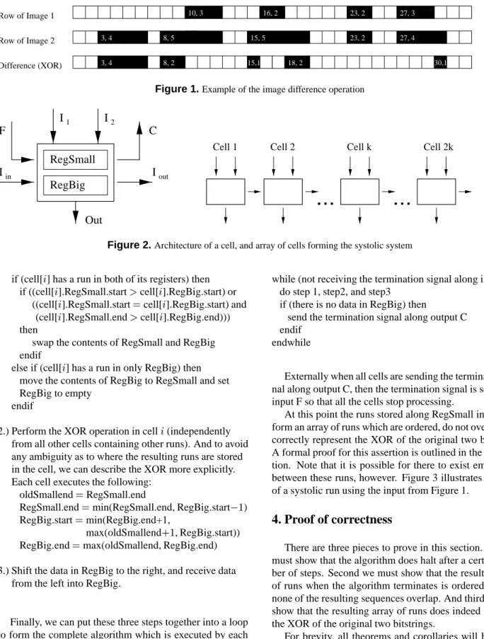
An example image difference operation is shown in fig-ure 1.

When using run-length encoding, the two inputs and the output are represented as arrays of 2-tuples of integers. In each tuple the first element is the start of the run and the second element is the run’s length. Each array of tuples must use a strictly increasing sequence of first elements of the tuples. By definition none of the intervals represented by the tuples for a single bitstring may overlap. In the input it is permissible, in general, for two intervals in a single bit-string to be directly adjacent to each other, and in the output

it is possible for this to occur as well, however an additional pass can be made at the end to ensure the encoding is com-pletely compressed. Note that only the foreground pixels are represented in the encoding.

The sequential algorithm for finding the image differ-ence of two RLE encoded bitstrings is a single pass through the two arrays simultaneously which merges them together into a single RLE encoded bitstring. We start at the begin-ning of the two arrays, and for each iteration we determine the XOR of the top run of both bitstrings, take the smaller of the resulting runs, and leave the remainder in the array it came from. This algorithm clearly has a time complexity of

O(

k

) where

k

is the number of runs in the two images. Also

it should be noted that this time complexity is the same for the best, worst, and average case.

3. RLE based systolic image difference

algo-rithm

If we let

k

be an upper bound on the number of runs in a

single input bitstring then the XOR operation can clearly not

produce more than2

k

runs, thus our systolic architecture

will use2

k

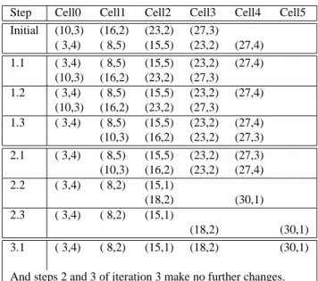
cells. Each cell will have two registers each

capable of storing two integers to represent a run, as shown in figure 2. Initially the first register of each cell will be used to store the array of runs representing the first image, and the second register of each cell will store the array of runs for the second image. After the algorithm has terminated, the first register of the cells will represent the result of the XOR operation and the second register of all cells will be empty.

For notation we will call the first register RegSmall and the second register RegBig. Also we will refer to runs by their starting and ending points rather than the starting points and lengths which are actually stored. Thus if cell

i

contains two runs where the first one starts at location 10

and has length 5 and the second one starts at location 12 and has length 8, our notation will indicate this as

cell[i].RegBig.start = 10

cell[i].RegBig.end = 14

cell[i].RegSmall.start = 12

cell[i].RegSmall.end = 19

Now we will describe the main steps of the algorithm which will be put into a loop to form the final algorithm. These steps will be executed by each cell individually, and

are written below to be executed by an arbitrary cell

i

.

Steps used in main algorithm:

1.) The purpose of this step is to put the ”smaller” run into RegSmall and the ”bigger” run into RegBig.

2 3 5 6 7 8 9 10 11 12 13 14 15 16 17 18 19 20 21 22 23 24 25 26 27 28 29 30 31 32 1 4 Difference (XOR) Row of Image 2 Row of Image 1 10, 3 16, 2 23, 2 27, 3 3, 4 8, 5 15, 5 23, 2 27, 4 3, 4 8, 2 15,1 18, 2 30,1

Figure 1.Example of the image difference operation

Cell 1 Cell 2 Cell k Cell 2k

out F I_in I I I C 1 2 RegSmall RegBig Out

Figure 2.Architecture of a cell, and array of cells forming the systolic system

if (cell[

i

] has a run in both of its registers) then

if ((cell[

i

].RegSmall.start

>

cell[

i

].RegBig.start) or

((cell[

i

].RegSmall.start=cell[

i

].RegBig.start) and

(cell[

i

].RegSmall.end

>

cell[

i

].RegBig.end)))

then

swap the contents of RegSmall and RegBig endif

else if (cell[

i

] has a run in only RegBig) then

move the contents of RegBig to RegSmall and set RegBig to empty

endif

2.) Perform the XOR operation in cell

i

(independently

from all other cells containing other runs). And to avoid any ambiguity as to where the resulting runs are stored in the cell, we can describe the XOR more explicitly. Each cell executes the following:

oldSmallend=RegSmall.end

RegSmall.end=min(RegSmall.end, RegBig.start,1)

RegBig.start=min(RegBig.end+1,

max(oldSmallend+1, RegBig.start))

RegBig.end=max(oldSmallend, RegBig.end)

3.) Shift the data in RegBig to the right, and receive data from the left into RegBig.

Finally, we can put these three steps together into a loop to form the complete algorithm which is executed by each cell

i

.

Algorithm for cell i:

while (not receiving the termination signal along input F) do step 1, step2, and step3

if (there is no data in RegBig) then

send the termination signal along output C endif

endwhile

Externally when all cells are sending the termination sig-nal along output C, then the termination sigsig-nal is sent along input F so that all the cells stop processing.

At this point the runs stored along RegSmall in the cells form an array of runs which are ordered, do not overlap, and correctly represent the XOR of the original two bitstrings. A formal proof for this assertion is outlined in the next sec-tion. Note that it is possible for there to exist empty cells between these runs, however. Figure 3 illustrates the steps of a systolic run using the input from Figure 1.

4. Proof of correctness

There are three pieces to prove in this section. First we must show that the algorithm does halt after a certain num-ber of steps. Second we must show that the resulting array of runs when the algorithm terminates is ordered and that none of the resulting sequences overlap. And third we must show that the resulting array of runs does indeed represent the XOR of the original two bitstrings.

For brevity, all theorems and corollaries will be stated, but the complete proofs will be omitted. They can be found in the technical report [12].

Step Cell0 Cell1 Cell2 Cell3 Cell4 Cell5 Initial (10,3) (16,2) (23,2) (27,3) ( 3,4) ( 8,5) (15,5) (23,2) (27,4) 1.1 ( 3,4) ( 8,5) (15,5) (23,2) (27,4) (10,3) (16,2) (23,2) (27,3) 1.2 ( 3,4) ( 8,5) (15,5) (23,2) (27,4) (10,3) (16,2) (23,2) (27,3) 1.3 ( 3,4) ( 8,5) (15,5) (23,2) (27,4) (10,3) (16,2) (23,2) (27,3) 2.1 ( 3,4) ( 8,5) (15,5) (23,2) (27,3) (10,3) (16,2) (23,2) (27,4) 2.2 ( 3,4) ( 8,2) (15,1) (18,2) (30,1) 2.3 ( 3,4) ( 8,2) (15,1) (18,2) (30,1) 3.1 ( 3,4) ( 8,2) (15,1) (18,2) (30,1)

And steps 2 and 3 of iteration 3 make no further changes.

Figure 3.Execution of the systolic algorithm on the in-puts from figure 1.

4.1. Proof for termination

The first part is quite trivial to show by induction. We will use the following two corollaries which lead directly to our first theorem.

Corollary 1.1: At the end of iteration

i

, the first

i

cells do not have any runs stored in RegBig [12].

Corollary 1.2: At no point in the algorithm will there

exist a non-empty cell beyond location

k

1+

k

2where

k

1is the number of runs in the first image and

k

2is

the number of runs in the second image [12].

Theorem 1 The systolic XOR algorithm terminates after at

most

k

1+

k

2steps.

Proof of termination: By corollary 1.1, after iteration

k

1+

k

2, the first

k

1+

k

2cells have no runs stored in RegBig. By

corollary 1.2 there are no non-empty cells beyond location

k

1+

k

2. Thus by iteration

k

1+

k

2the only non-empty

cells are ones which have no runs stored in RegBig, which means that the termination condition is satisfied by iteration

k

1+

k

2.2

4.2. Proof for proper ordering

In this section we prove that the resulting array of runs when the algorithm terminates is ordered and that none of the resulting sequences overlap. This part takes somewhat longer to prove than the termination, however the basic idea is only a slight refinement over brute force. First we will

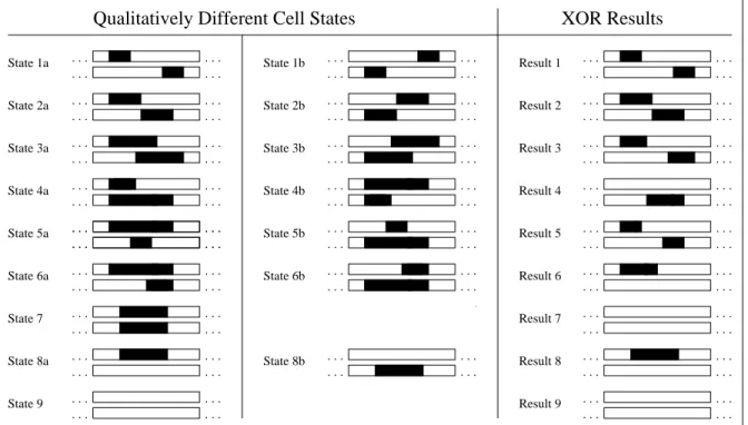
introduce some more notation to more easily refer qualita-tively to all the various possible states a cell can be in. These states are shown in figure 4.

The first two columns of figure 4 show all the possible cell states, and the third column shows the result of per-forming steps 1 and 2 on each of these cells. The reason for the pairings between columns 1 and 2 is that the “a” states and the “b” states are related in the sense that any “b” state will turn into the corresponding “a” state after step 1 is per-formed, and any “a” state will be unchanged by a step 1.

We wish to prove that the runs stored along RegSmall and RegBig of the cells are always ordered. More specifi-cally, we show the following.

Theorem 2 At the end of every iteration, for every cell

i

, and every

j

to its right(

j > i

),

1. if both cells

i

and

j

contain runs in RegSmall, then cell[

i

].RegSmall.end

<

cell[

j

].RegSmall.start, and 2. if both cells

i

and

j

contain runs in RegBig, then

cell[

i

].RegBig.end

<

cell[

j

].RegBig.start.

We can write the theorem in a format more conducive to proof as follows. Since each iteration of the algorithm consists of three steps and the third is so simple, we fo-cus the corollary below on the first two steps. For

nota-tion we refer to the state of cell

i

before an iteration

be-gins as cell[

i

].before, and the state of the cell after the first,

second, and third steps as cell[

i

].after1, cell[

i

].after2, and

cell[

i

].after3 respectively. Note that the current iteration

is not included because it would unduly clutter the nota-tion. Thus the iteration being considered must be made clear from context.

Corollary 2.1: At any iteration, for every cell

i

, and for every cell

j

to its right(

j > i

),

1. if both cells

i

and

j

contain runs in RegSmall after

step 2, then cell[

i

].after2.RegSmall.end is less than

cell[

j

].after2.RegSmall.start,

2. if both cells

i

and

j

contain runs in RegBig

af-ter step 2, then cell[

i

].after2.RegBig.end is less than

cell[

j

].after2.RegBig.start,

3. if cell

i

has a run in RegSmall and in RegBig

af-ter step 2, then cell[

i

].after2.RegSmall.end is less than

cell[

i

].after2.RegBig.start,

4. if cell

i

has a run in RegSmall and cell

j

has one in

RegBig after step 2, then cell[

i

].after2.RegSmall.end

is less than cell[

j

].after2.RegBig.start, and

5. If after step 3 some cell

k

between cells

i

and

j

(including

i

itself) has no run in RegSmall, and if

cell

i

has a run in RegBig and cell

j

has a run in

RegSmall, then cell[

i

].after3.RegBig.end is less than

. . . . . . . . . . . . . . . . . . . . . . . . . . . . . . . . . . . . . . . . . . . . . . . . . . . . . . . . . . . . . . . . . . . . . . . . . . . . . . . . . . . . . . . . . . . . . . . . . . . . . . . . . . . . . . . . . . . . . . State 7 State 2a State 4a State 5a State 6a State 9 State 8a State 3a . . . . . . . . . . . . . . . . . . . . . . . . . . . . . . . . . . . . . . . . . . . . . . . . . . . . . . . . . . . . . . . . . . . . . . . . . . . . . . . . . . . . State 1a . . . . . . . . . . . . State 1b State 2b State 3b State 4b State 5b State 6b State 8b Result 1 Result 5 Result 9 Result 8 Result 7 . . . . . . . . . . . . . . . . . . . . . . . . . . . . . . . . . . . . . . . . . . . . . . . . . . . . . . . . . . . . . . . . . . . . . . . . . . . . . . . . . . . . . . . . . . . . . . . . Result 2 Result 3 Result 4 Result 6

Qualitatively Different Cell States

XOR Results

Figure 4.List of qualitatively different cell states.

Note that parts three, four and five of the above corol-lary are included only because they are useful in proving the induction step. The proof of corollary 2.1 is by induc-tion on the number of iterainduc-tions and can be found in our technical report [12]. The first four parts are reasonably in-tuitive, however the fifth part may not be. In the proof given in the technical report, the first four parts follow rather di-rectly from some simple inequalities which involve break-ing a brute force approach into several cases in which all the possibilities fall, while the fifth part requires more reason-ing.

Once corollary 2.1 is proven, it is fairly easy to show theorem 2:

Proof of theorem 2: Execution of step 3 of the

algo-rithm does not have any effect on the truth of the first part of corollary 2.1. Thus if the first inequality from corollary 2.1

is shown to be true between cells

i

and

j

after steps 1 and 2

are performed, then the first part of theorem 2 is true too. If

part two of the corollary is shown to be true between cells

i

and

j

after steps 1 and 2, then part one of the theorem is true

for all cells

i

+1and

j

+1, which covers all pairings which

do not use the first cell. And since RegBig of this first cell

is empty, the pairings involving it are vacuously true.2

4.3. Correctness proof for the resulting RLE string

To conclude the formal proof of correctness for our sys-tolic algorithm, we need to show that the resulting array of

runs does indeed represent the XOR of the original two bit-strings. This part is rather easy compared to the previous section. The idea is to view the runs of the two bitstrings as a set of many distinct smaller bitstrings and observe that the only changes made to this set involve XORs among these bitstrings. This combined with the fact that XOR is asso-ciative imply that the final state is the correct XOR of the original two bitstrings.

In more detail, the definition of the image difference

problem was given as difference[

i

] = img1[

i

]img2[

i

], for

each

i

in the range1to

b

, whererepresents the

exclusive-or operation, and where

b

is the number of pixels in the

image.

We can easily extend this to apply to a set of bitstrings instead of merely two bitstrings. We could write this as

difference

[

i

]= 8 > > > > < > > > > : 0

if anevennumberof

bitstringsfromthesethavea

oneinbiti; or

1

if anoddnumberof bitstrings

fromthesethaveaoneinbiti:

For two bitstrings these are clearly equivalent definitions of the difference. For any set of bitstrings, we will view the difference of the entire set according to the definition above. To make this definition useful we must make the obser-vations that

Corollary 3.1: if the runs of a bitstring are viewed as a set of smaller bitstrings, then the XOR of this set is the original bitstring [12], and

Corollary 3.2: letting xor(A) represent the result of XORing the bitstrings contained in the set A, we have

for arbitrary sets of bitstrings A and B that xor(A[B)

=xor(fxor(A), xor(B)g) [12].

Now we wish to use these corollaries to prove that the image difference produced by the algorithm is correct.

Theorem 3 The image difference produced by the systolic

algorithm is the same as the correct XOR defined in section 2.

Proof of correctness: We can let A be the set of runs

contained in the first image, and let B be the set of runs in the second image. Thus based on our first observation, xor(A) is the first image and xor(B) is the second image, so the final result we seek is xor(xor(A), xor(B)), which

ac-cording to our second observation is equal to xor(A[B).

Now that we have expressed the desired result as an XOR over the set of all runs contained in the two images, we must show that although the set of runs being considered changes at each step of the algorithm, the resulting XOR is still the same after each iteration.

Clearly steps 1 and 3 of a given iteration do not change the set of runs under consideration. Only the second step causes any changes. And since XOR is an associative

oper-ation, we can say that xor(A[B) is xor(A[xor(B)) by an

argument very similar to the one used in our second obser-vation above. Letting B be a pair of runs XORed in a cell during step 2, we see that the XOR of the set of runs before step 2 is the same as the XOR of the new set of runs after step 2. Thus we have now shown that at any point in the algorithm, if C is the set of runs contained in the systolic system, then xor(C) is the correct XOR (i.e. xor(xor(A), xor(B))). And due to theorems 1 & 2, when the iterations are over, the final result will be stored in RegSmall in a sorted and non-overlapping manner, thus making xor(C) equal to the bitstring represented directly by the runs of C. That is, the bitstring stored in the end is indeed the correct XOR.

5. Algorithm performance

In this section we present experimental results to show that the systolic algorithm obtains the final result very quickly when the bitstrings being XORed are highly sim-ilar. More specifically, the time for the systolic algorithm is proportional to the difference between the number of runs in the two images for similar images. In contrast the time for the sequential algorithm is proportional to the total number of runs in the two images together.

First another upper bound can be put on the number of steps the algorithm will take. When we proved termination

above, we showed it would stop in at most

k

1+

k

2steps

where

k

1is the number of runs in the first bitstring, and

k

2is the number of runs in the second bitstring. We also

believe that it is bounded by the number of runs in the image difference, although we have not yet proven this.

Observation: If the runs of the two input bitstrings are

encoded such that none of the runs are adjacent (in other words if the bitstring is compressed as much as possible), then the systolic XOR algorithm terminates after at most

k

3+1steps, where

k

3is the number of runs in the output

from the systolic algorithm (note the output from the sys-tolic algorithm will not always be compressed as much as possible).

If we let the similarity of two images be measured by the number of runs in the final result, then the above observa-tion implies that the systolic algorithm has the potential to run faster the more similar two bitstrings are.

A simulation program was written to test the algorithm on a large number of randomly generated input cases. The size for the image rows was varied from 128 to 2048 pixels. The “on” pixels in the first image were chosen in runs of length 4 to 20, and the second image was obtained by flip-ping some of the bits of the first image in either direction (1 to 0, and 0 to 1). Here these changes are called “errors” and they were created in runs of length 2 to 6. The percentage of “on” pixels in the first image and of the errors in the second image was varied by changing the average distance between the runs.

The empirical testing shows that for medium amounts of error (when the number of pixels changed was less than 30% of the total image) the dominating factor was the dif-ference between the number of runs in the two images. This was true irrespective of the sizes of the images and varied only slightly over different densities.

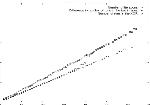
This is demonstrated in figure 5, which shows the aver-age number of iterations taken by the algorithm as a func-tion of the percentage of pixels with errors. The other two sets of data show the average difference in the number of runs in the two images, which correlate very closely with the number of iterations up through 30–40%, and the num-ber of runs in the XOR produced by the algorithm which is the upper bound we have not proven yet.

In the figure below the image size is 10,000 pixels with approximately 250 runs in the original image, which trans-lates to a density of 30%. The pattern is similar for smaller images, but the variation is higher.

In explanation of the high correlation between the num-ber of iterations taken and the difference in the numnum-ber of runs in the two images, we notice that after the first itera-tion the larger number of runs will be stored along RegS-mall. Then if the shift-right procedure in step 3 causes a

0 500 1000 1500 2000 2500 0 10 20 30 40 50 60 70

Percent of pixels that are different between the two images

Number of iterations Difference in number of runs in the two images Number of runs in the XOR

Figure 5.Number of iterations as a function of the percent of pixels with errors plotted along side two of the dominating factors in the algorithms running time.

run to be pushed into this group of runs along the end, then all the runs at the end will need to be pushed to the right a cell. And clearly the number of steps taken by this chain reaction will be the length of this group of runs at the end, which is the difference between the number of runs in the two images.

When the number of pixels changed is much greater than 30% of the total image, a different factor begins to domi-nate. For the smaller amounts of difference there will be lots of empty cells left behind throughout the array, thus the only significant data movement will be at the end as discussed in the previous paragraph. But as the number of differences increases and thus the number of empty cells decreases, more and more data movement will be required thus pushing the algorithm closer to the upper bound.

The previous figure demonstrates the correlation be-tween the number of iterations taken by the algorithm and the difference in the number of runs in the two images and it demonstrates an upper bound as the number of runs in the XOR after the algorithm finishes, however it does not give a good impression of the algorithms speed. This can be seen in the next table which focuses on smaller amounts of error. Table 1 shows the average number of iterations taken by both the sequential and the systolic algorithm on an image of size ranging from 128 to 2048 pixels. In the first case, the errors are kept at approximately 3.5% of the image, thus causing both the systolic and the sequential versions to take

linearly more time as the image size increases. In the second case however, the number of errors is fixed at 6 runs each of size 4 pixels, thus while the sequential algorithm still takes large amounts of time, the systolic algorithm averages just over 5 iterations regardless of how large the image gets.

Algorithm Errors Iterations versus image size 128 256 512 1024 2048 Systolic 3.5% 1.8 2.8 4.7 8.6 16.6 Sequential 3.5% 4.9 9.5 18.8 37.8 75.9 Systolic 6 runs 5.3 5.4 5.5 5.7 5.8 Sequential 6 runs 8.3 12.3 19.7 34.9 65.1

Table 1.Average systolic iterations versus sequential iter-ations for small amounts of errors (where the length of runs in images is 4–20, and the length of error runs is 2–6).

6. Conclusions and future research

This paper has shown that a systolic array can perform an image difference operation on RLE encoded images very quickly if the two images are highly similar. Indeed, the number of iterations taken is bounded above by the number of runs left in the XOR, and for similar images the number

of iterations is tightly correlated with the difference between the number of runs in the two images.

Although a parallel solution of the image difference problem can easily be performed on uncompressed data in constant time if the number of processors available is pro-portional to the number of pixels in the images, there is no known parallel algorithm which performs the same opera-tion in compressed mode. To the best of our knowledge this paper demonstrates the first effective parallel solution which operates on compressed data directly. This method has the advantage of using a smaller number of processors, and it does not require the time to convert the image between RLE format and bitmap mode.

In both the case of highly similar and highly different images, the number of iterations taken seems to be domi-nated by the frequent need to push a whole set of runs to the right to make room for a new entry. If a broadcast bus existed which could run at the same frequency as the rest of the systolic system, it might be possible to perform these shifts more efficiently thus significantly decreasing the run-ning time. Thus one area of future research should be mod-ifying the algorithm to run more quickly on a model with a fast broadcast bus, such as a reconfigurable mesh [13]. Ad-ditionally, the task of combining the adjacent runs in differ-ent cells at the end of the algorithm is left as future research. This task also is not fast on a pure systolic system, but could be performed quickly with the help of a broadcast bus.

References

[1] P. P. Jonker and E. R. Komen, “A scalable real-time image processing pipeline,” Proceedings. 11th

IAPR International Conference on Pattern Recogni-tion, 1992, Vol. IV. Conference D: Architectures for

Vision and Pattern Recognition, p. xvii+243, 142-6. [2] F. Ercal et al., “A fast modular RLE-Based inspection

scheme for PCBs,” Proc. of SPIE - Architectures,

Net-works, and Intelligent Systems for Manufacturing In-tegration, Pittsburgh, Oct. 1997, Vol. 3203, pp. 49-59.

[3] S. Gil, R. Milanese, and T. Pun, “Comparing features for target tracking in traffic scenes,” Pattern

Recogni-tion, 1996, vol.29, no.8, p. 1285-96

[4] H. Kawasumi, H. Sekii, N. Enomoto, H. Ohata, and A. Okazaki, “Detecting intruders using time-series data by projection pattern of silhouette,” Electrical

Engi-neering in Japan, 1997, vol.119, no.1, p. 62-73

[5] G. M. Emelyanov, N. V. Kurmyshev, and O. Y. Yu-vzhik, “Procedures and algorithms for detecting and determining the orientation of objects in binary im-ages,” Pattern Recognition and Image Analysis, 1997, vol.7, no.3, p. 373-8

[6] G. Agam, J. Frydman, O. Amiram, and I. Dinstein, “Efficient morphological processing of maps and line-drawings based on directional interval coding,”

Pro-ceedings of the SPIE - The International Society for Optical Engineering, 1997, vol.3168, p. 41-51.

[7] N. K. Ratha, A. K. Jain, and D. T. Rover, “Convolu-tion on Splash 2,” Proc. Of IEE Symposium on FPGAs

for Custom Computing Machines, Napa Valley, CA,

April, 1995.

[8] A. Rasquinha and N. Ranganathan, “C3L: A Chip for Connected Component Labelling,” IEEE 10th

Inter-national Conf. on VLSI Design, January 1997,

pp.446-51.

[9] M. Djunatan and T. Mengko, “A programmable real-time systolic processor architecture for image mor-phological operations, binary template matching and min/max filtering,” 1991 IEEE International

Sympo-sium on Circuits and Systems, p. 5 vol. xlviii+3177,

65-8 vol.1, 1991.

[10] N. Ranganathan, and K. B. Doreswamy, “A Sys-tolic Algorithm and Architecture for Image Thinning,”

Proc. Of Fifth Great Lakes Symoisium on VLSI,

Buf-falo, NY, Mar. 1995

[11] Vipin Kumar et al., Introduction to Parallel

Comput-ing: Design and Analysis of Algorithms, The

Ben-jamin/Cummings Publishing Company Inc. 1994.

[12] F. Ercal, M. Allen, and H. Feng, Proof of

Cor-rectness and Performance Analysis of a Systolic Image Difference Algorithm for RLE-Compressed

Images Technical Report CSc 99-01,

Univer-sity of Missouri – Rolla, 1998. [Also available at

http://www.cs.umr.edu/˜mallen/research/csc99-01.ps] [13] Y. Ben-Asher, D. Peleg, R. Ramaswami, and A. Schuster, “The power of reconfiguration,” J. Parallel