Structured and Sparse Signal Estimation

(1)

Fundamental Limits and Error Bounds

A THESIS

SUBMITTED TO THE FACULTY OF THE GRADUATE SCHOOL OF THE UNIVERSITY OF MINNESOTA

BY

Akshay Soni

IN PARTIAL FULFILLMENT OF THE REQUIREMENTS FOR THE DEGREE OF

Doctor of Philosophy

Prof. Jarvis Haupt

(2)

c

(3)

Acknowledgements

The very old Chinese proverb “The fragrance always remains in the hand that gives roses”, very rightly captures my thoughts while writing this thesis. I would have never seen this day without the many who constantly guided, supported, loved and respected me. I wish to thank all of them from the bottom of my heart.

I begin by thanking god for providing me the ability, “India” for allowing me to dream globally and “The United States of America” for providing me the opportunity to accomplish my dreams.

I would like to thank my parents, whose love for each other and for the family inspired me at every step of life. In particular, I would like to thank my mother Mrs. Anjana Soni for her everlasting support and constant motivation, and my father Mr. Vijay Soni for teaching me the value of being organized and honest. I would never forget the sacrifices you have made for my future, and I would try my level best to keep you happy.

I would like to thank my sisters Aditi and Bharti for their love and for allowing me to share my emotions at hard times with them. I would also like to thank my brothers Gaurav and Alish for being my best friends for all these years and for all the memories we have made together.

Thank you my late sister Rekha – I am sure if you were with us, you would have been very happy with my achievements. I miss you!

I owe a major part of my gratitude to my Ph.D. advisor, Jarvis Haupt, for believing in me, for supporting me throughout my graduate school. I would always feel proud of being your Ph.D. student and more than that, your first Ph.D. student. I would consider myself extremely lucky if I can be half as down to earth and approachable as you are. Positivity, honesty and hard work are the traits which I have learnt from you

(4)

me to work and grow together with you. I would also like to acknowledge and express my gratitude for financial support from Defense Advanced Research Projects Agency, National Science Foundation, and the University of Minnesota, Twin Cities.

I would like to thank Prof. Keshab Pahri for being my academic advisor during first year of school and for introducing me to Jarvis.

I would like to thank my committee members – Prof. Georgios Giannakis, Prof. Nikos Sidiropoulos, and Prof. Arindam Banerjee – for their time and consideration, and for the many fruitful suggestions to improve my quality of work.

I would like to thank my lab mates – Swayambhoo Jain, Sirisha Rambhatla, Xingguo Li, Mojtaba Kadkhodaie Elyaderani, Di Xiao, Scott Sievert and Alex Gutierrez – for the enlightening discussions and other fun activities. I would specially like to thank Swayambhoo and Sirisha for the much needed coffee breaks and the most entertaining political discussions (and sometimes work too!).

I would like to thank Dr. Fatih Porikli (MERL) for offering me an internship while we met during ICASSP 2012. It was a great learning experience and helped me to see the potentials of my research in practical scenarios.

I would also like to thank GraphLab for getting me in touch with Dr. Debora Donato (StumbleUpon). I would like to thank Debora for allowing me to work within her group as an intern. It was a great experience and I am looking forward to work with you in future.

I would like to thank Quresh, Gaurav, and Aritra for being great roommates and friends – there are a lot of memories with you that I will cherish for life. Thank you Ashutosh and Amrita for being the awesome couple they are – your love and support is truly a factor in this milestone of mine. Thanks to all my friends – Shraddha, Shivani, Prashant, Vikas, Vishal, Saunil, Sanika and Parita – for the good times that we shared in Minneapolis.

Finally, I would like to thank my best friend and my wife Tanvi Sharma, for her love and care, for accepting me as I am, and for her constant support. I am truly blessed to have you as my life partner.

(5)

Dedication

To my mother Mrs. Anjana Soni – eagerness of whom to see me succeed, kept me motivated to do hard work.

(6)

Abstract

Over the past decade, sparsity has become one of the most prevalent themes in signal processing and Big-Data applications. In general, sparsity describes the phenomenon where high-dimensional data can be explained by only a few variables, values, or coeffi-cients. The presence of sparsity often enables efficient algorithms for extracting relevant information from the data. This effort focuses on the theoretical treatment of special-ized sensing and inference techniques that exploit sparsity and other forms of structured low-dimensional representations.

The first part of this work focuses on noisy matrix estimation and completion prob-lems. We consider the problem of estimating matrices that adhere to a “sparse-factor model” decomposition – matrices that may be accurately described by a product of two matrices, one of which is sparse – from noisy observations, where the noise is modeled as random and may arise from any of a number of various likelihood models (e.g., Gaus-sian, Poisson, Laplace, and even one-bit models). Sparse-factor models can be used to describe collections of vectors that reside in a union of linear subspaces, and can be viewed as a powerful generalization the widely-used principal component analysis technique, which assumes data reside on or near a single subspace. We establish es-timation error guarantees for sparse-factor matrix eses-timation problems (where a noisy observation of each matrix entry is observed) and matrix completion problems (where only a subset of elements is observed, each corrupted by noise), and describe an efficient algorithm for performing inference in problems of this form.

In the second part of this work, we examine and quantify the benefits of “adaptive sensing” techniques, which employ data-dependent feedback in the data acquisition process, in the context of a structured sparse inference task. This work is motivated by a desire to formally exploit the structural characteristics and dependencies present in the wavelet representations of many natural images. We devise an efficient and provably-optimal (in a minimax sense) adaptive acquisition method for estimating the locations of the significant wavelet coefficients from noisy observations. Our results demonstrate the significant improvements that can be obtained when leveraging the inherent structural dependencies in the sparse representation of the signal to be acquired and incorporating

(7)

either structural information or adaptivity alone. Overall, our results provide essential new insights into the virtues of adaptive data acquisition in sparse inference tasks.

(8)

List of Tables

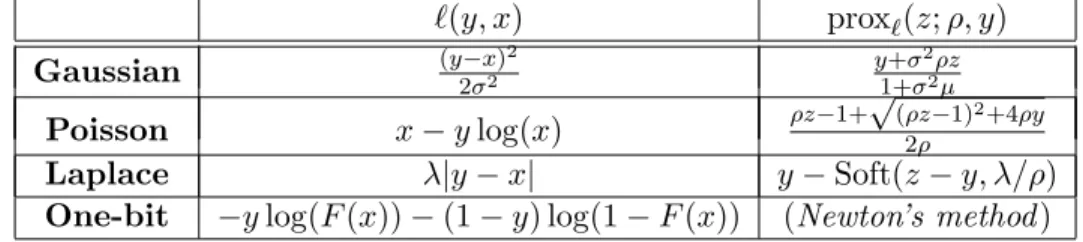
3.1 Expressions for prox_`(z;ρ, y) = arg minx∈_R `(y, x) +ρ₂(x−z)2 for

differ-ent `(y, x), corresponding to negative log-likelihoods for the models we examine. Here, forλ >0, soft(x, λ) = sgn(x) max{|x| −λ,0}. . . 44 3.2 Experimental parameters for different likelihood models we examine. Here

X∗_min= mini,jX_i,j∗ and X_max∗ =kX∗kmax. . . 47

4.1 Summary of necessary conditions for exact support recovery using non-adaptive or non-adaptive sensing strategies that obtain m measurements of k-sparsen-dimensional signals that are either unstructured or tree sparse in an underlying nearly complete binary tree. For each setting, we state the critical value of µ such that whenever µ is smaller than a constant times the stated quantity, the minimax risk over the class of signalsXµ,k of the form (4.8) will be strictly bounded away from zero. . . 89

(12)

List of Figures

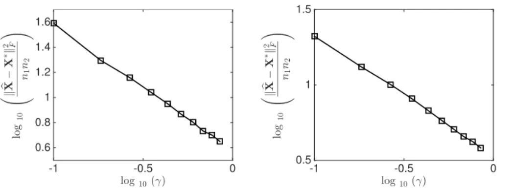
3.1 Results of synthetic experiments for matrix completion with Gaussian, Laplace and Poisson likelihoods: —-—- is Gaussian, − −_♦ − − is Laplace, and —-◦—- is Poisson. Top row corresponds to sparse-factor model with k = 8 while the bottom row corresponds to weak-lp model withp= 1/3. Column 1 corresponds toσ2= (0.5)2(for Laplaceτ =√8), column 2 corresponds to σ2 _{= (1)}2 _{(for Laplace} _τ ₌√_{2) and column 3}

corresponds to σ2 = (2)2 (for Laplace τ = 1/√2). Here n1 = 100,

n2 = 1000 andr = 20. . . 48

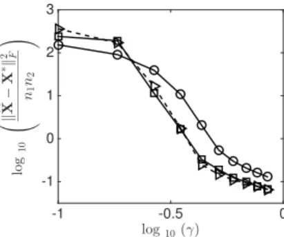
3.2 Results of synthetic experiments for one-bit matrix completion under sparse factor models, using the logistic link function. The left panel corresponds to the case where theA∗ matrix is exactly sparse; the right when columns ofA∗ lie in a weak-lp ball withp= 1/3. . . 49 3.3 Comparison between sparse-factor and nuclear-norm-regularized matrix

completion methods. The curves are: our proposed procedure with `0

regularizer (), the `1 regularized variant of our approach (B), and

nu-clear norm regularized low-rank matrix completion (◦). The sparse fac-tor completion methods perform similarly, and both achieve a lower er-ror than the best nuclear-norm regularized estimate for sampling rates γ ≥10−0.5 ≈30%. . . 52 4.1 A signal x∈_R7 _{(left) that is 4-tree sparse in an underlying binary tree}

having 7 nodes (right). The supportS(x) ={1,2,3,5}corresponds to a rooted connected subtree of the underlying tree. . . 80

(13)

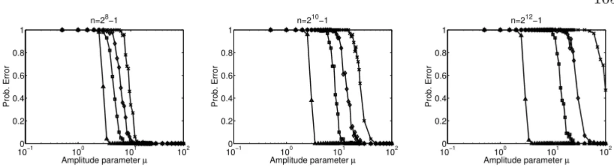
plitude parameterµin three different problem dimensionsn. In each case, four different sensing and support recovery approaches – the adaptive tree sensing procedure described here (4markers); the adaptive compressive sensing approach of [158] (markers); a Group Lasso approach for recov-ering tree-sparse vectors (markers), and a Lasso approach for recovering unstructured sparse signals (×markers) – were employed to recover the support of a tree-sparse signal with 16 nonzeros of amplitude µ. The proposed tree-sensing procedure outperforms each of the other methods, and exhibits performance that is unchanged as the problem dimension increases. . . 105 4.3 Empirical probability of successful support recovery for the tree-sensing

procedure of Algorithm 4 as a function of signal sparsityk and squared signal component amplitude µ2, for a fixed measurement budget. Here, the light and dark regions correspond to settings where the empirical probability of correct support recovery (averaged over 100 trials) is nearly one or nearly zero, respectively. The dashed line corresponds to the threshold above which our theoretical results guarantee correct support recovery with probability at least 0.99. The empirical results here ap-pear to validate our theoretical predictions for this scenario (see text for specific simulation details). . . 107

(14)

Chapter 1

Introduction

Over the past decade, sparsity has become one of the most prevalent themes in signal processing and Big-Data applications. In general sparsity describes the phenomenon where high-dimensional data can be explained by only a few variables or values. The notion of sparsity enforces a small number of degrees of freedom in the otherwise high-dimensional data – potentially leading to efficient algorithms to extract relevant infor-mation without wasting expensive and often-scare resources.

Geometrically, sparsity forces a high-dimensional signal (or vector) to lie in a low-dimensional subspace of the high-low-dimensional space. To be precise, let an-dimensional signal be k-sparse (i.e., only k out of its n entries are nonzero) in the canonical (i.e., identity) basis. The canonical basis vectors corresponding to the nonzero entries of the signal defines the basis for the k-dimensional subspace in which thisn-dimensional signal resides. It is then clear that a k-sparse n-dimensional signal can belong to any one of the n_k k-dimensional linear subspaces of Rn. Any recovery procedure will have

to allocate some resources for each of these subspaces. A small k (i.e., more sparsity) then would reduce the candidate number of subspaces, thus enabling us to recover the relevant information either by using less resources or more efficiently by allocating the available resources only to a small number of subspaces.

Structured sparsity refers to sparse representations that are drawn from a restricted union of subspaces where only a subset of n_k

subspaces are allowable. The advantages are clear – if we can exploit the structure information then we can use the available resources more judiciously and no allocation of resources would be required for the

(15)

subspaces which are not allowed. Several procedures have been developed which takes the advantage of the underlying sparsity structure and provides accurate recovery with either less resources or efficient algorithms or both [128–130].

Active research areas like image processing, machine learning, speech processing, compressive sensing (CS), radar signal processing, genomics, network sciences, nuclear medicine, medical imagining and wireless communications, have all received a revived interest due to advances in sparsity guided state-of-the-art algorithms and applications. The focus has been on the theoretical treatment of techniques that exploit sparsity (or structured sparsity) in problems involving high-dimensional data, along with practical data acquisition methods – be it non-adaptive sampling like in CS or adaptive sampling (sampling with feedback) like in many recent works on adaptive CS [1–4]. This work makes a leap forward by studying implications of different kinds of structure (and spar-sity) assumptions that can be imposed on the data along with their intimate interplay with corresponding adaptive sampling and recovery methods.

The first part of this work focuses on noisy matrix estimation and completion prob-lems. We consider the problem of estimating matrices that adhere to a “sparse-factor model” decomposition – matrices that may be accurately described by a product of two matrices, one of which is sparse – from noisy observations, where the noise is modeled as random and may arise from any of a number of various likelihood models (e.g., Gaus-sian, Poisson, Laplace, and even one-bit models). Sparse-factor models can be used to describe collections of vectors that reside in a union of linear subspaces, and can be viewed as a powerful generalization the widely-used principal component analysis technique, which assumes data reside on or near a single subspace. We establish es-timation error guarantees for sparse-factor matrix eses-timation problems (where a noisy observation of each matrix entry is observed) and matrix completion problems (where only a subset of elements is observed, each corrupted by noise), and describe an efficient algorithm for performing inference in problems of this form.

Specifically, in Chapter-2, we provide guarantees for the denoising problem where we get Poisson distributed samples of all the entries of the matrix. We formulate sparse and structured dictionary-based Poisson denoising problem as a constrained maximum likelihood estimation problem, and establish performance bounds for their mean-square

(16)

estimation error using the framework of complexity penalized maximum likelihood anal-yses. Our results [5] provides theoretical foundations to existing dictionary learning

based experimental Poisson denoising procedures.

A follow-on effort, extends this problem to the case of missing-data where we only get to observe a subset of entries of the matrix of interest. We extend our Poisson denoising analyses to missing data case and provide performance bounds for a variety of noise models. This work appears as Chapter-3.

The second part of this thesis studies the problem of support recovery (locations of the nonzero elements) of tree-sparse signals from noisy linear measurements. We propose a simple structured-adaptive support recovery procedure and provide sufficient condition on the signal amplitude in order to recover the exact support of a tree-sparse signal with high probability. We further establish fundamental performance limits for the task of support recovery of tree-sparse signals from noisy measurements, in settings where measurements may be obtained either non-adaptively (using a randomized Gaus-sian measurement strategy motivated by initial CS investigations) or by any adaptive sensing strategy. Our main results imply that the proposed adaptive tree sensing pro-cedure is nearly optimal, in the sense that no other sensing and estimation strategy can perform fundamentally better for identifying the support of tree-sparse signals. This work establishes that the combination of structure and adaptivity is a powerful one and for some structures (like tree) both the necessary and sufficient conditions are indepen-dent of ambient dimension and only depends on the sparsity level. This work appears as Chapter-4.

In Chapter-5, several future directions are discussed along with some concluding remarks.

(17)

Advances in Structured Matrix Recovery

This part contains two contributions to the matrix recovery problem. Our specific focus is on settings where the matrix to be estimated is well-approximated by a product of two (a priori unknown) matrices, one of which is sparse. Such structural models – referred to here as “sparse factor models” – have been widely used, for example, in subspace clustering applications, as well as in contemporary sparse modeling and dictionary learning tasks.

Chapter-2 is a reprint of our IEEE International Symposium on Information Theory paper [5]. This work provides a theoretical foundation for the experimentally stud-ied Poisson denoising tasks using dictionary learning approach [6, 7], where underlying structural assumption on data is of a sparse factor model. Specifically, we formu-late sparse and structured dictionary-based Poisson denoising methods as constrained maximum likelihood estimation strategies, and establish performance bounds for their mean-square estimation error using the framework of complexity penalized maximum likelihood analysis.

Chapter-3 examines a general class of noisy matrix completion tasks where the goal is to estimate a matrix with sparse factor model from observations obtained at a subset of its entries, each of which is subject to random noise or corruption. Our main theoretical contributions are estimation error bounds for sparsity-regularized maximum likelihood estimators for problems of this form, which are applicable to a number of different observation noise or corruption models. This work has been submitted to the IEEE Transactions on Information Theory, and is currently under review [8].

(18)

Chapter 2

Estimation Error Guarantees for

Poisson Denoising with Sparse

and Structured Dictionary

Models

Poisson processes are commonly used models for describing discrete arrival phenomena arising, for example, in photon-limited scenarios in low-light and infrared imaging, as-tronomy, and nuclear medicine applications. In this context, several recent efforts have evaluated Poisson denoising methods that utilize contemporary sparse modeling and dictionary learning techniques designed to exploit and leverage (local) shared structure in the images being estimated. This work establishes a theoretical foundation for such procedures. Specifically, we formulate sparse and structured dictionary-based Poisson denoising methods as constrained maximum likelihood estimation strategies, and estab-lish performance bounds for their mean-square estimation error using the framework of complexity penalized maximum likelihood analyses.1

1

The material in Chapter-2 is c2014 IEEE. Reprinted, with permission, fromIEEE International Symposium on Information Theory, “Estimation Error Guarantees for Poisson Denoising with Sparse and Structured Dictionary Models,” A. Soni and J. Haupt.

(19)

2.1

Introduction

Across a broad range of engineering application domains, Poisson processes have been utilized to describe discrete event or arrival phenomena. For example, in a host of imaging applications (including infrared and thermal imaging, night vision, astronomical imaging, and nuclear medicine, to name a few) the random arrival of photons at each detector in an array may be modeled using Poisson-distributed random variables, with unknown rates or intensities. A fundamental problem in these applications is that of estimating the unknown rates associated with each of the sources, a task typically referred to as Poisson denoising.

We consider here a denoising task along these lines. Suppose that we are equipped with a collection of detectors, and that the arrival of photons at each individual detector may be accurately described by a Poisson process with some unknown (non-negative) rate. At each detector we acquire a single integer-valued observation, corresponding to the number of photons arriving at the detector over some fixed (but not necessarily specified) time interval that we assume to be the same across all detectors. It follows that the observation at each detector is a Poisson-distributed random variable whose parameter is the product of the underlying rate parameter of the process and the length of the time interval (see, e.g., [9]). We assume the Poisson processes giving rise to the observations at each detector are mutually independent.

Suppose that there are a total of d detectors. For each ` ∈ [d] where [d] is short-hand for the set {1,2, . . . , d}, we denote the Poisson-distributed observation at the `-th detector as y` and denote by x∗` its unknown parameter. Letting Poi(y`|x∗`) = (x∗_`)y`_exp(₋_x∗

`)/(y`)! denote the univariate Poisson probability mass function (pmf) defined on nonnegative integers y` ∈N0, we may write the joint pmf of thed

observa-tions, defined on Nd0, as

p({y`}`∈[d]|{x∗`}`∈[d]) =

Y

`∈[d]

Poi(y`|x∗`), (2.1)

where the product form on the right-hand side follows from our independence assump-tion on the individual Poisson processes.

(20)

2.1.1 Exploiting Data Structure in Poisson Denoising Tasks

In the absence of any structural dependencies among the collection of rates {x∗_`}_`∈[d],

the Poisson denoising task is somewhat trivial – in this case, classical estimation theo-retic analyses establish that each observation is itself the minimum variance unbiased estimator of its underlying parameter (see, e.g., [10]). More interesting approaches to the denoising task, then, seek to exploit some form of underlying structure among the individual rates. Efforts along these lines include [11, 12], which proposed and analyzed estimation strategies applicable in scenarios where the collection of rates (appropriately arranged) admits a simple representation in terms of a wavelet representation, and [13], which also examined multiresolution representations of the collection of rates. Along similar lines, the work [14] analyzed estimation procedures tailored to signals that are sparse (or nearly so) in any orthonormal basis, within the context of a compressed sensing approach to the Poisson denoising problem.

A number of related efforts have examined Poisson denoising tasks using data repre-sentations or bases that are learned from the data themselves, in contrast to the efforts described above that utilize fixed bases or representations. Such “data-driven” esti-mation strategies include Poisson-specific extensions of classical methods like principal component analysis and other matrix factorization methods [15, 16], as well as applica-tion of contemporary ideas from sparse dicapplica-tionary learning [17–19] to Poisson-structured data [20]. We note, in particular, the recent works [7] and [6], which describe estimation tasks employing models that may be described as sparse or structured dictionary-based models; our effort here is motivated by a desire to provide theoretical justification for these dictionary-based techniques.

2.1.2 Our Approach

The sparse and structured dictionary-based models upon which our analyses are based describe underlying data structure in terms of matrix factorization models. To that end, we will find it useful here to formulate our model so that the collection ofdobservations are interpreted as elements of an m×n matrix (with d = mn) denoted by Y, and having elements Yi,j, where for i ∈[m] and j ∈ [n], Yi,j is a Poisson random variable with rateX_i,j∗ . LettingX∗ be the m×nmatrix with entriesX_i,j∗ , we overload (slightly)

(21)

the notation in (2.1), and write the joint pmf of the observations in this case as p(Y|X∗) = Y

i∈[m],j∈[n]

Poi(Yi,j|Xi,j∗ ),Poi(Y|X∗). (2.2)

Our interest here is primarily on settings where the matrixX∗ admits a dictionary-based factorization, so that X∗ = D∗A∗, where D∗ ∈ Rm×p and A∗ ∈ Rp×n. Since

such factorization models are themselves fairly general, we restrict our attention here to two specific settings – the first being when the matrix A∗ is sparse so that only a small fraction of its elements are nonzero (along the lines of models employed in dictionary learning efforts), and the second when p, the number of columns of D∗

and rows of A∗, is small relative to m and n (in which case X∗ admits a low-rank

decomposition). That said, the analytical approach we develop here is fairly general, and thus may readily be extended to other factorization models (e.g., non-negative matrix factorization, structured dictionary models, etc.).

The estimation approaches we analyze here amount to constrained maximum likeli-hood estimation procedures. Abstractly, we consider a set X of candidate estimatesX

forX∗, each of which admits a factorization of the formX=DA. The elements of the factors D and A may themselves be constrained to enforce the type of structure that we assume present in X∗. Formally, we construct sets CD and CA and a set

X _,

X=DA :D∈CD, A∈CA, max

i,j |Xi,j| ≤Xmax

where 0<Xmax<∞ is a constant that describes the maximum rate of the underlying

processes (and whose specific role will become evident in our analysis), and we consider estimatesXb of X∗ constructed according to

b

X= arg min

X∈X−logp(Y|X) +λpen(X), (2.3)

where pen(X) is a non-negative penalty that quantifies the inherent “complexity” of each estimate X∈ X, and λ >0 is a user-specified regularization parameter. For both the low-rank and the sparse dictionary based models we consider here, we describe the construction of suitable sets CDand CA, cast each corresponding estimation procedure

in terms of an optimization of the form (2.3) (with appropriately constructed penalties), and derive mean-square estimation error rates using analysis techniques motivated by those employed in [13, 14, 21–26].

(22)

2.1.3 Related Efforts in Poisson Restoration

While our focus here is on Poisson denoising, we briefly note several related efforts that examine restoration and deblurring methods for Poisson-distributed data [27–31]. These works employ regularized maximum likelihood estimation strategies similar in form to those we analyze in this effort. More recently, [32] proposed a dictionary-based approach to the Poisson deblurring task.

2.1.4 Organization and Notation

The remainder of this paper is organized as follows. We present our main theoretical results, stated in terms of the estimation procedures proposed in [6, 7], in Section 2.2, and provide proofs in Section 2.3. In Section 2.4 we briefly discuss how our analytical approach overcomes somewhat limiting minimum rate assumptions inherent in several prior works that use penalized maximum likelihood methods for Poisson denoising. In Section 2.5, we conclude with a discussion of potential extensions of our analysis.

A brief note on notation employed in the sequel – for a matrix A, we denote its number of nonzero elements by kAk₀, the sum of absolute values of its elements by

kAk1, and its dimension (the product of its row and column dimensions) by dim(A).

For an integer m∈_N, the notation1m denotes an all-ones lengthm column vector.

2.2

Main Results

As noted above, our analyses here are motivated by recent efforts ( [6, 7]) that examine Poisson denoising tasks arising in imaging problems and provide empirical evaluations of procedures that exploit local shared structure in the rates being estimated. These prior works each utilize “patch-level” structural models for the underlying image, in which the shared structure arises in terms of factorizations of matrices comprised of vectorized versions of small image patches.

The first procedure proposed in [7] is a non-local variant of a principal component analysis (PCA) method. That approach uses an initial clustering step designed to iden-tify collections of similar patches, then obtains estimates of the underlying rate functions of the image by performing low-rank factorizations of patch-level matrix representations

(23)

of each data cluster. In terms of our model here, the approximation step inherent to this approach may be described by assuming the true matrix of ratesX∗ ∈Rm×ngiving

rise to independent Poisson-distributed observations Y in each data cluster admits a decomposition of the form X∗ = D∗A∗, where D∗ ∈ _Rm×p _and _A∗ _∈

Rp×n for some

p≤min(m, n).

Both [7] and [6] also examine sparse dictionary-based denoising methods along the lines of recent efforts in the dictionary learning literature (see, e.g. [19]), which seek to model the image patches as sparse linear combinations of columns of a learned dictionary matrix. Here, this model assumes that the true rate matrix X∗ admits a decomposition of the formD∗A∗ whereA∗ is sparse (e.g., having fewer than somekmax non zeros per

column). Sparse dictionary-based models may be interpreted as a natural extension of low-rank models; the latter essentially fits the data to a single low-dimensional linear subspace, while the former utilizes a union of linear subspaces.

Our main results establish mean square error guarantees for estimates for these tasks that are obtained via penalized maximum likelihood estimation strategies. In order to state our results, we need to first construct a set X of candidate reconstructions, with appropriate penalties. To that end, we fix parameters Amax > 0, and Xmax > 0, and

λ0 >1, let q be a positive integer satisfying

q ≥max 4,3 + log 18Amax λ0_log(2) ,1 + log 36Amax Xmax , (2.4)

and letLbe the smallest integer exceeding (max(m, n))q. Now, for any positive integer p ≤ min(m, n) we let X be the set of candidate reconstructions of the form X =DA

satisfying maxi,j|Xi,j| ≤ Xmax, where D ∈ D are in Rm×(p+1) and A ∈ A are in R(p+1)×n, so that each entry ofDtakes values on one ofLuniformly-spaced quantization

levels in the range [−1,1] and each element of A takes on one of L possible uniformly spaced quantization levels in the range [−Amax, Amax].

Our first result, stated here as a theorem, pertains to sparse dictionary-based models.

Theorem 2.2.1. Let the true rate matrixX∗ be m×n, wheremax(m, n)≥3. Suppose X∗ satisfies the constraint maxi,jX_i,j∗ <Xmax/2, and admits a dictionary-based decom-position of the form D∗A∗, where the dictionary D∗ is m×p for p < n with entries bounded in magnitude by 1, and the coefficient matrix A∗ is p×n whose elements are

(24)

bounded in magnitude by Amax. Let observations Y of X∗ be acquired according to the model (2.2).

Form the setX as above, and letpen(X) = [q·dim(D)+(q+2)·kAk0]·log(max(m, n)). The estimate Xb = Xb(Y) = DbAb formed using the solution of the penalized maximum

likelihood problem

{Db,Ab}= arg min

D∈CD,A∈CA:DA∈X

−logp(Y|DA) +λkAk₀, (2.5)

withλ=λ0·(q+2)·log(max(m, n)) log(2)(and whereλ0 is as specified in the construction of X) satisfies E h kX∗−Xbk2_F i mn λ0Xmax m(p+ 1) mn + kA∗k0+n mn log(max(m, n)).

Here, the expectation is with respect to the distribution of Y parameterized by the true rate matrix X∗, and the notation suppresses leading (finite, positive) constants.

The salient take-away point here is that the average per-element estimation error is upper bounded by a term that decays essentially in proportion to the number of “degrees of freedom” in the model divided by the number of observations. In other words, our result here establishes that the estimation error exhibits characteristics of the well-known parametric rate.

The result of Thm. 2.2.1 also provides guidance on when dictionary-based estimation procedures are viable. Consider, for example, a setting where the true matrix A∗ in the dictionary-based decomposition ofX∗ has somekmaxnonzero elements per column.

Here, Theorem 2.2.1 establishes that the mean-square estimation error for estimating

X∗ decays in proportion to (p+ 1)/n+ (kmax+ 1)/m, ignoring leading constants and

logarithmic factors. This result implies natural conditions on the estimation task – that accurate estimation is possible when the number of columns of X∗ exceeds (by a multiplicative constant times a factor logarithmic in the dimension) the number of true dictionary elements p, and the number of rows of X∗ exceeds (by a multiplicative constant times a factor logarithmic in the dimension) the number of non zeros in the sparse representation of each column. This latter condition is reminiscent of conditions arising in compressive sensing (see, e.g., [26, 33, 34]).

(25)

We obtain an analogous result for the case where the true rate matrixX∗ admits a low-rank decomposition. We state the result here as a corollary of Theorem 2.2.1.

Corollary 2.2.1. Suppose that max(m, n) ≥ 3, and that the true rate matrix X∗ ∈

Rm×n admits a low-rank decomposition, so that it may be written asX∗ =D∗A∗, where

D∗ is m×p and A∗ is p×n with p≤min(m, n), and such that X_i,j∗ ≤Xmax/2, ∀i, j. Let observations Y be acquired via the model (2.2). Form the set X as above, and let

pen(X) = [q·dim(D) + (q+ 2)·dim(A)]·log(max(m, n)).

The estimateXb =Xb(Y) =DbAb formed using the solution of the following penalized

maximum likelihood problem

{Db,Ab}= arg min D∈CD,A∈CA:DA∈X −logp(Y|DA), (2.6) satisfies E h kX∗−Xbk2_F i mn λ 0_X max (p+ 1)(m+n) mn log(max(m, n)),

where as above the expectation is with respect to the distribution of Y parameterized by the true rate matrix X∗, and the notation suppresses leading (finite) constants.

Note that in this case the penalty pen(X) is actually the same for all X∈ X, as it depends only on the dimensions of the two factors, which are the same for all candidates by construction of X. Thus, the estimation approach here reduces to just a maximum likelihood estimation over constrained sets. As above, the estimation error rate exhibits characteristics of the parametric rate, as the low-rank model here has O(p(m+n)) degrees of freedom.

2.3

Proofs of Main Results

We write pXi,j(·) as shorthand for the scalar Poisson pmf with rateXi,j, and we denote the multivariate Poisson pmfp(·|X) defined in (2.2) (parameterized by the collection of rates {Xi,j}i,j) by pX(·).

Central to our analysis will be the aforementioned countable sets X of candidate reconstructions of the unknown (non-negative) rate matrixX∗. We consider setsX con-structed as above, and assign to eachX∈ X a non-negative “penalty” quantity denoted

(26)

by pen(X) (which here will quantify the “complexity” of the corresponding estimate), so that the collection of penalties satisfies the summability condition P

X∈X2−pen(X)≤1.

Note that this condition is just the Kraft-McMillan inequality; in constructing penalties for elements of X we will employ the well-known fact that the Kraft-McMillan inequal-ity is satisfied provided we may construct a uniquely decodable code for the elements

X∈ X; see [35]. With this, we begin by establishing a fundamental result, from which our results follow.

Lemma 2.3.1. Suppose that the elements of the unknown non-negative rate matrixX∗ are bounded in amplitude, so that for some fixed Xmax>0, we have 0≤X_i,j∗ ≤Xmax/2 for all i∈[m]and j∈[n]. LetX be a countable set of candidate solutions Xsatisfying the uniform bound maxi∈[m],j∈[n]|Xi,j| ≤ Xmax, with associated non-negative penalties

{pen(X)}_X∈X satisfying the Kraft-McMillan inequality as stated above. Collect a total of mn independent Poisson measurements Y = {Yi,j}_i∈[m],j∈[n], parameterized by X∗, according to the model (2.2). If there exists X+ ∈ X such that X_i,j+ −X_i,j∗ ≥ 0 for all

i ∈[m] and j ∈ [n], then for any choice of λ0 >1, the complexity penalized maximum likelihood estimate b X= arg min X∈X {−logp(Y|X) +λ 0 log(2)·pen(X)}, (2.7) satisfies, E h kX∗−Xbk2_F i mn ≤ 4Xmax mn kX∗−X+k1+λ0log(2)·pen(X+) , (2.8)

where the expectation is taken with respect to the distribution of Y ∼pX∗.

Proof. Our proof utilizes a straight-forward extension of a result stated and utilized in [13,14] (based on the essential ideas of [24,36]), which we provide here without proof: for any λ0 >1 the complexity regularized maximum likelihood solution Xb of the form

(2.7), obtained by optimizing over any countable set X of candidates having penalties

{pen(X)}_X∈X satisfying the Kraft-McMillan inequality, satisfies

−2Elog A(pX∗, p b

X)≤_Xmin_∈X

(27)

where the expectation is with respect to the distribution of Y∼pX∗. Here, K(pX∗, p_X), X Y∈_Nm×n 0 log p(Y|X∗) p(Y|X) p(Y|X∗)

denotes the Kullback-Leibler divergence (or KL divergence)2 of pX frompX∗, and the quantity A(pX∗, p b X), X Y∈_Nm×n 0 q p(Y|X∗₎_·_p(_Y_| b X)

is the Hellinger Affinity between pX∗ and p b

X. Now, since the upper bound in (2.9) holds for X ∈ X which achieves the minimum, it holds for all X ∈ X. Considering, specifically, the estimatorX+∈ X, we have

−2Elog A(pX∗, p b

X)≤K(pX∗, pX+) +λ

0_log(2)_·_pen(_X+_). _(2.10)

Specializing to the Poisson case, we use the results of Lemmas 2.3.2 and 2.3.3 (in Section 2.3.3) to obtain, respectively, a lower bound for the left-hand side and an upper bound for the right-hand side of (2.10). The result follows.

Our main results of Section 2.2 follow from specializing this result to each of the two structural models. We establish first a proof of the sparse dictionary-based inference estimation procedure; the analogous result for estimation in low-rank models follows as a simple corollary.

2.3.1 Proof of Theorem 2.2.1

The proof of our first main result follows directly from Lemma 2.3.1 above. First, note that each candidate estimate X = DA ∈ X may be described via a code, in which each element of D is encoded using log(L) = qlog(max(m, n)) bits and each nonzero element of A is encoded using log(dim(A)) bits to denote its location, and log(L) bits for its amplitude. Thus, a total of q ·dim(D)·log(max(m, n)) bits suffice to encode

D, and since log(dim(A))<log(max(m, n)2_{), matrices}_A _having_k_A_k

0 nonzero entries 2

Note that the KL divergence is only well-defined here for non-negativeX, when the corresponding Poisson pmf p(Y|X) is well-defined. We make no specific constraint here that each X ∈ X be non-negative, but without loss of generality we may take K(pX∗_{, p}_{X) to be infinite also when} _X_{has any} non-negative entries. Further, note the KL divergence is infinite here if for anyi, j,Xi,j= 0 butXi,j∗ 6= 0 (i.e., when the distributionpX∗is not absolutely continuous with respect topX).

(28)

can be described using no more than kAk₀ ·(q + 2)·log(max(m, n)) bits. Overall, this implies we may choose pen(X) = q ·dim(D)·log(max(m, n)) +kAk0 ·(q + 2)·

log(max(m, n)). Note that while constructing the codes we did not care about the uniform bounded condition (i.e., that each entry should be bounded by Xmax); in effect,

we formed uniquely decodable codes for a bigger set X0 such thatX ⊆ X0, so we always have P

X∈X2−pen(X) ≤

P

X∈X02−pen(X)≤1.

Now, consider a candidate reconstruction of the form XQ = DQAQ+1m(α1Tn) , ˜

DQA˜Q, whereDQ and AQ are the closest quantized surrogates of the true parameters

D∗ and A∗, and 0 ≤α≤Amax is a quantity to be specified. Denote DQ =D∗+4D and AQ=A∗+4A, where4D and4A are the quantization error matrices. Then, it is easy to see that

˜

DQA˜Q−D∗A∗=1m(α1Tn) +D∗4A+4DA∗+4D4A. (2.11) To satisfy the conditions of Lemma 2.3.1, we must have that XQ overestimates (element-wise) the true rate matrix, and that the right-hand side of (2.11) be no larger than Xmax/2. To that end, our aim is to choose α so that the right side of (2.11)

becomes element-wise nonnegative, but no larger than Xmax/2. It is straightforward

to see that each entry of the matrices D∗4A and 4DA∗ is bounded in magnitude by 2pAmax/L. Also, the elements of the matrix 4D4A are bounded in magnitude by 4pAmax/L2 ≤ 4pAmax/L. Thus, it suffices to choose α as the smallest quantization

level exceeding 8pAmax/L to ensure the each element of the matrix on the right-hand

side of (2.11) is nonnegative. Since we choose α to be the higher quantization level of 8pAmax/L, and the quantization levels for elements ofA are of size 2Amax/L, we have

that α≤(8p+ 2)Amax/L. In order for α to be a valid entry ofA, it must be bounded

by Amax, which is true whenever L≥(8p+ 2).

We can now bound each entry of ˜DQA˜Q−D∗A∗ as follows ( ˜DQA˜Q−D∗A∗)i,j = (1m(α1n)T +D∗4A+4DA∗+4D4A)i,j ≤ (8p+ 2)Amax L + 2pAmax L + 2pAmax L + 4pAmax L = 16pAmax L + 2Amax L ≤ 18pAmax L ,

(29)

where the second inequality follows from bounds on the entries of each matrix mentioned above and the last inequality is valid for p≥1. This quantity is no larger than Xmax/2

whenever L≥36pAmax/Xmax, and in this case, we ensure that XQ∈ X.

Now, note thatkX∗−XQk1 =Pi∈[m],j∈[n]( ˜DQA˜Q−D∗A∗)i,j ≤18p·(mn)·Amax/L,

and if we now evaluate the oracle bound (2.8) from Lemma 2.3.1 at the candidate XQ which overestimates X∗ (entry-wise), we have

E h kX∗−Xbk2_F i mn ≤ 4Xmax mn kX∗−XQk1+λ0log(2)·pen(XQ) ≤ 72pXmaxAmax L +λ 0_·_{4 log(2)X} max· pen(XQ) mn ≤λ0·8 log(2)Xmax· pen(XQ) mn ,

where the last line follows whenever L ≥ 18Amax_λ0_log(2)mnp (since pen(XQ) corresponds to a binary code having length greater than 0, we have pen(XQ)≥1).

Overall, then, the result follows since by construction, we have dim(De_Q)≤mp+m,

and kAe_Qk₀≤ kA∗k₀+n, and the assumption (2.4) implies

L≥max 8p+ 2,18Amaxmnp λ0log(2) , 36pAmax Xmax . 2.3.2 Proof of Corollary 2.2.1

The proof of Corollary 2.2.1 follows directly from the proof of Theorem 2.2.1 – in particular, by substituting kA∗k0 =pn.

2.3.3 Useful Lemmata

The following lemmata are used in the proof of Lemma 2.3.1.

Lemma 2.3.2 (From [14]). For any two (non-negative) Poisson rate matrices Xa and Xb, having entries uniformly bounded above byXmax, we have

1 4Xmax

(30)

Lemma 2.3.3. For non-negative Poisson rate matrices Xa and Xb such thatXb over-estimates Xa element-wise i.e., X_i,jb −X_i,ja ≥ 0 for all i ∈ [m] and j ∈ [n], we have

K(pXa, p_Xb)≤ kXb−Xak1.

Proof. By independence and the definition of the KL divergence, K(pXa, p_Xb) = X i∈[m],j∈[n] " X_i,ja logX a i,j X_i,jb +X b i,j−Xi,ja # ≤ X i∈[m],j∈[n] h X_i,jb −X_i,ja i =kXa−Xbk1,

where the inequality follows from the fact that X_i,ja logX a i,j Xb

i,j

≤0 sinceX_i,jb ≥X_i,ja (and following standard convention that alog(a/0) =∞,0 log(0/a) = 0 for a >0).

2.4

Discussion

It is worthwhile to explicitly point out a unique point in our analysis – introducing the additional dimension in the model to ensure that our class of candidate solutions contains an element that always overestimates, element-wise, the rates in the true pa-rameter matrix X∗ – enables us to obtain estimation error rates without making any assumptions on the minimum rate of the underlying Poisson processes. This is a signif-icant contrast with prior efforts employing penalized maximum likelihood analyses (but with different structural models) on Poisson-distributed data [13,14], each of which pre-scribe adopting an assumption that the rates associated with each Poisson-distributed observation be strictly bounded away from 0.

Our extension here is an important advance, especially in the context of extremely photon-limited scenarios. Indeed, in these settings it is somewhat counter-intuitive (or at least, restrictive) to assume that the rates be bounded away from zero, as it is precisely in these scenarios when one might be most interested in estimating rates that are very near zero. Further, classical analyses suggest that there may be no fundamental reason why zero or nearly-zero rates become more difficult to estimate. For instance, in the scalar Poisson rate estimation problem, the Cramer-Rao lower bound for estimating a Poisson rate parameter from n iid Poi(·|θ) observations (achievable with the sample average estimator) is θ/n, suggesting that the estimation problem actually becomes easier as

(31)

the rate decreases. The analytical framework we develop here facilitates analysis of these important low-rate cases under sparse and structured data model assumptions.

Finally, we note that Poisson models also find utility other application domains beyond imaging. In networking tasks, for example, Poisson processes are a natural choice to model arrival events, such as packets arriving at each of a number of network routers our flows across network links (see, e.g., [37]). Our techniques and analysis here would extend directly to other application domains, as well.

2.5

Conclusions

In this work, we described a framework for quantifying the mean-square error of con-strained maximum likelihood Poisson denoising strategies, in settings where the collec-tion of underlying rates (appropriately arranged) admits a low-rank or sparse diccollec-tionary- dictionary-based decomposition. We established that, in these cases, the mean-square estimation error exhibits characteristics of the familiar parametric rate, in that the error essentially takes the form of “degrees of freedom” divided by “number of observations.” In analogy to related analyses in [14, 26], our analysis can also be used to obtain error rates for data adhering to models that are not exactly sparse, but instead are characterized by coefficients whose ordered amplitudes decay (e.g., at a polynomial rate). Finally, while our analysis here was formulated in terms of matrix-structured data and factorization models, these methods may be extended straightforwardly to encompass also sparse and low-rank models for higher-order tensor structure data. We defer in-depth investigations of these extensions to a future effort.

(32)

Chapter 3

Noisy Matrix Completion under

Sparse Factor Models

This work [8] examines a general class of noisy matrix completion tasks where the goal is to estimate a matrix from observations obtained at a subset of its entries, each of which is subject to random noise or corruption. Our specific focus is on settings where the matrix to be estimated is well-approximated by a product of two (a priori unknown) matrices, one of which is sparse. Such structural models – referred to here as “sparse factor models” – have been widely used, for example, in subspace clustering applications, as well as in contemporary sparse modeling and dictionary learning tasks. Our main theoretical contributions are estimation error bounds for sparsity-regularized maximum likelihood estimators for problems of this form, which are applicable to a number of different observation noise or corruption models. Several specific implications are examined, including scenarios where observations are corrupted by additive Gaussian noise or additive heavier-tailed (Laplace) noise, Poisson-distributed observations, and highly-quantized (e.g., one-bit) observations. We also propose a simple algorithmic approach based on the alternating direction method of multipliers for these tasks, and provide experimental evidence to support our error analyses.

(33)

3.1

Introduction

In recent years, there has been significant research activity aimed at the analysis and development of efficient matrix completion methods, which seek to “impute” missing elements of a matrix given possibly noisy or corrupted observations collected at a subset of its locations. Let X∗∈_Rn1×n2 _{denote a matrix whose elements we wish to estimate,}

and suppose that we observe X∗ at only a subsetS ⊂[n1]×[n2] of its locations, where

[n1] ={1,2, . . . , n1} is the set of all positive integers less or equal to n1 (and similarly

forn2), obtaining at each (i, j)∈ S a noisy, corrupted, or inexact measurement denoted

by Yi,j. The overall aim is to estimateX∗ givenS and the observations{Yi,j}₍_i,j₎∈S. Of

course, such estimation problems may be ill-posed without further assumptions, since the values of X∗ at the unobserved locations could in general be arbitrary. A common approach is to augment the inference method with an assumption that the underlying matrix to be estimated exhibits some form of intrinsic low-dimensional structure.

One application where such techniques have been successfully utilized is collabo-rative filtering (e.g., as in the well-known Netflix Prize competition [38]). There, the matrix to be estimated corresponds to an array of users’ preferences or ratings for a col-lection of items (which could be quantized, e.g., to one of a number of levels); accurately inferring missing entries of the underlying matrix is a useful initial step in recommend-ing items (here, movies or shows) to users deemed likely to rate them favorably. A popular approach to this problem utilizes a low-rank modeling assumption, which im-plicitly assumes that individual ratings depend on some unknown but nominally small number (say r) of features, so that each element of X∗ may be described as an inner product between two length-r vectors – one quantifying how well each of the features are embodied or represented by a given item, and the other describing a user’s affinity for each of the features. Recent works examining the efficacy of low-rank models for matrix completion include [39–45].

Several other applications where analogous ideas have been employed, but which leverage different structural modeling assumptions, include:

• Sparse Coding for Image Inpainting and Demosaicing: Suppose that the underlying data to be estimated takes the form of an n1×n2 color image, which

(34)

three color planes). The image inpainting task amounts to estimating the image from a collection of (possibly noisy) observations obtained at individual pixel locations (so that at each pixel, either all or none of the color planes are observed), and the demosaicing task entails estimating the image from noisy measurements corresponding to only one of the 3 possible color planes at each pixel. The recent work [46] proposed estimation approaches for these tasks that leveragelocal shared structure manifesting at the patch level. Specifically, in that work, the overall image to be estimated is viewed equivalently as a matrix comprised of vectorized versions of its small (e.g., 5×5×3 or 8×8×3) blocks, and the missing values are imputed using a structural assumption that this patch-based matrix be well-approximated by a product of two matrices, one of which is sparse.

• Sparse Models for Learning and Content Analytics: A recent work [47] in-vestigated a matrix completion approach to machine-based learning analytics. There, the elements of then1×n2 matrix to be estimated, sayX∗, are related to

the probability with which one of n1 questions will be answered correctly by one

of n2 “learners” through a link function Φ : R→ [0,1], so that the value Φ(Xi,j∗ ) denotes theprobability with which questioniwill be correctly answered by learner j. The observed data are a collection of somem < n1n2 binary values, which may

be interpreted as (random) Bernoulli(Φ(X_i,j∗ )) variables. The approach proposed in [47] entails maximum-likelihood estimation of the unknown latent factors ofX∗, under an assumption thatX∗ be well-approximated by a sum of two matrices, the first being product of a sparse non-negative matrix (relating questions to some latent “concepts”) and a matrix relating a learner’s knowledge to the concepts, and the second quantifying the intrinsic difficulty of each question.

• Subspace Clustering from Missing Data: The general subspace clustering problem entails separating a collection of data points, using an assumption that similar points are described as points lying in the same subspace, so that the overall collection of data are represented as points belonging generally to a union of (ostensibly, low-dimensional) subspaces. This general task finds application in image processing, computer vision, and disease detection, to name a few (see, e.g., [48–53], and the references therein). One direct way to perform clustering in

(35)

such applications entails approximating the underlying matrixX∗ whose columns comprise the (uncorrupted) data points by a product of two matrices, the second of which is sparse, so that the support (the set of locations of the nonzero elements) of each column of the sparse matrix factor identifies the subspace to which the corresponding column ofX∗ belongs.

While these examples all seem qualitatively similar in scope, their algorithmic and analytical tractability can vary significantly depending on the type of structural model adopted. In the collaborative filtering application, for example, a desirable aspect of adopting low-rank models is that the associated inference (imputation) procedures can be relaxed to efficient convex methods that are amenable to precise performance analy-ses. Indeed, the statistical performance of convex methods for low-rank matrix comple-tion are now well-understood in noise-free settings (see, e.g., [39–42]), in settings where observations are corrupted by some form of additive uncertainty [54–58], and even in settings where the observations may be interpreted as nonlinear (e.g., highly-quantized) functions of the underlying matrix entries [59–61]. In contrast, the aforementioned in-ference methods based on general bilinear (and sparse) factor models are difficult to solve to global optimality, and are instead replaced by tractable alternating minimiza-tion methods. More fundamentally, the statistical performance of inference methods based on these more general bilinear models, in scenarios where the observations could arise from general (perhaps nonlinear) corruption models or could even be multi-modal in nature, has not (to our knowledge) been fully characterized.

This work provides some initial results in this direction. We establish a general-purpose estimation error guarantee for matrix completion problems characterized by any of a number of structural data models and observation noise/corruption models. For concreteness, we instantiate our main result here for the special case where the matrix to be estimated adheres to asparse factor model, meaning that it is well-approximated by the product of two matrices, one of which is sparse (or approximately so). Sparse factor models are inherent in the modeling assumptions adopted in the aforementioned works on image denoising/demosaicing, content analytics, and subspace clustering, and are also at the heart of recent related efforts in dictionary learning [17–19]. Sparse factor models may also serve as a well-motivated extension to the low-rank models often utilized in collaborative filtering tasks. There, while it is reasonable to assume

(36)

that users’ preferences will depend on a small number of abstract features, it may be that any particular user’s preference relies heavily on only a subset of the features, and that the features that are most influential in forming a rating may vary from user to user. Low rank models alone are insufficient for capturing this “higher order” structure on the latent factors, while this behavior may be well-described using the sparse factor models we consider here.

3.1.1 Our Contributions

We address general problems of matrix completion under sparse factor modeling assump-tions using the machinery ofcomplexity-regularized maximum likelihoodestimation. Our main contributions come in the form of estimation error bounds that are applicable in settings where the available data correspond to an incomplete collection of noisy ob-servations of elements of the underlying matrix (obtained at random locations), and under general (random) noise/corruption models. We examine several specific implica-tions of our main result, including for scenarios characterized by additive Gaussian noise or additive heavier-tailed (Laplace) noise, Poisson-distributed observations, and highly-quantized (e.g., one-bit) observations. Where possible, we draw direct comparisons with existing results in the low-rank matrix completion literature, to illustrate the potential benefit of leveraging additional structure in the latent factors. We also propose an efficient unified algorithmic approach based on the alternating direction method of mul-tipliers [62] for obtaining a local solution to the (non-convex) optimizations prescribed by our analysis, and provide experimental evidence to support our error results.

3.1.2 Connections with Existing Works

As alluded above, our theoretical analyses here are based on the framework of complexity regularized maximum likelihood estimation [23,24], which has been utilized in a number of works to establish error bounds for Poisson estimation problems using multi scale models [13, 63], transform domain sparsity models [14], and dictionary-based matrix factorization models [5]. Here, our analysis extends that framework to the “missing data” scenarios inherent in matrix completion tasks (and also provides a missing-data extension of our own prior work on dictionary learning from 1-bit data [64]).

(37)

Our proposed algorithmic approach is based on the alternating direction method of multipliers (ADMM) [62]. ADMM-based methods for related tasks in dictionary learning (DL) were described recently in [65], and while our algorithmic approach here is qualitatively similar to that work, we consider missing data scenarios as well as more general loss functions that arise as negative log-likelihoods for our various probabilistic corruption models (thus generalizing these techniques beyond common squared error losses). In addition, our algorithmic framework also allows for direct incorporation of constraints not only on estimates of the matrix factors, but also on the estimate of

X∗ itself to account for entry-wise structural constraints that could arise naturally in many matrix completion scenarios. Several other recent efforts in the DL literature have proposed algorithmic procedures for coping with missing data [66, 67], and a survey of algorithmic approaches to generalized low-rank modeling tasks is given in the recent work [68].

Our inference tasks here essentially entail learning two factors in a bilinear model. With a few notable exceptions (e.g., low-rank matrices, and certain non-negative ma-trices [69–72]), the joint non-convexity of these problems can complicate their analysis. Recently, several efforts in the dictionary learning literature have established theoreti-cal guarantees on identifiability, as well as lotheoreti-cal correctness of a number of factorization methods [73–78], including in noisy settings [79]. Our efforts here may be seen as a complement to those works, providing additional insight into the achievable statistical

performance of similar methods under somewhat general noise models.

The factor models we employ here essentially enforce that each column of X∗ lie in a union of linear subspaces. In this sense our efforts here are also closely related to problems in sparse principal component analysis [80], which seek to decompose the (sample) covariance matrix of a collection of data points as a sum of rank-one factors expressible as outer products of sparse vectors. Several efforts have examined algorith-mic approaches to the sparse PCA problem based on greedy methods [81] or convex relaxations [82–84], and very recently several efforts have examined the statistical per-formance of cardinality- (or `0-) constrained methods for identifying the first sparse

principal component [85, 86]. These latter approaches are related to our effort here, as our analysis below pertains to the performance of matrix completion methods utilizing an `0 penalty on one of the matrix factors.

(38)

Finally, we note that problems of subspace clustering from missing or noisy data have received considerable attention in recent years. Algorithmic approaches to subspace clustering with missing data were proposed in [53, 87, 88], and several recent works have identified sufficient conditions under which tractable algorithms will provably recover the unknown subspaces in missing data (but noise-free) scenarios [89]. Robustness of subspace clustering methods to missing data, additive noise, and potentially large-valued outliers were examined recently in [52, 53, 90].

3.1.3 Outline

The remainder of this paper is organized as follows. Following a brief discussion of several preliminaries (below), we formalize our problem in Section 3.2 and present our main result establishing estimation error guarantees for a general class of estimation problems characterized by incomplete and noisy observations. In Section 3.3 we discuss implications of this result for several specific noise models. In Section 3.4 we discuss a unified algorithmic approach to problems of this form, based on the alternating direction method of multipliers, and provide a brief experimental investigation that partially validates our theoretical analyses. We conclude with a brief discussion in Section 3.5. Auxiliary material and detailed proofs are relegated to the appendix.

3.1.4 Preliminaries

To set the stage for the statement of our main result, we remind the reader of a few key concepts. First, recall that forp≤1 a vector x∈Rnis said to belong to a weak-`p ball

of radiusR >0, denotedx∈w`p(R), if its ordered elements|x(1)| ≥ |x(2)| ≥ · · · ≥ |x(n)|

satisfy

|x(i)| ≤Ri−1/p for alli∈ {1,2, . . . , n}, (3.1)

see e.g., [91]. Vectors in weak-`p balls may be viewed as approximately sparse; indeed, it is well-known (and easy to show, using standard results for bounding sums by integrals) that for a vector x∈w`p(R), the `q error associated with approximatingx by its best k-term approximation obtained by retaining its klargest entries in amplitude (denoted

(39)

here by x(k)) satisfies kx−x(k)kq, n X i=1 |xi−x(_ik)|q !1/q ≤R Cp,q k1/q−1/p, (3.2)

for any q > p, where Cp,q is given by

Cp,q= p q−p 1/q . (3.3)

For the special case q≥2p, we have Cp,q ≤1, and so

kx−x(k)kq ≤R k1/q−1/p. (3.4) We also recall several information-theoretic preliminaries. When p(Y) and q(Y) denote the pdf (or pmf) of a real-valued random variable Y, the Kullback-Leibler di-vergence (or KL didi-vergence) of q from pis denoted D(pkq) and given by

D(pkq) =Ep

logp(Y) q(Y)

where the logarithm is taken to be the natural log. By definition, D(pkq) is finite only if the support ofpis contained in the support ofq. Further, the KL divergence satisfies D(pkq) ≥ 0 and D(pkq) = 0 when p(Y) = q(Y). We also use the Hellinger affinity denoted by A(p, q) and given by

A(p, q) =Ep "s q(Y) p(Y) # =Eq "s p(Y) q(Y) #

Note that A(p, q)≥0 essentially by definition, and a simple application of the Cauchy-Schwarz inequality gives that A(p, q)≤1, implying overall that 0≤A(p, q)≤1. When p andq are parameterized by elementsXi,j and Xi,je of matricesXand Xe, respectively,

so that p(Yi,j) = pXi,j(Yi,j) and q(Yi,j) = qXei,j(Yi,j), we use the shorthand notation D(pXkqXe),

P

i,jD(pXi,jkqXei,j) and A(pX, qXe),

Q

i,jA(pXi,j, qXei,j).

Finally, for a matrix Mwe denote by kMk0 its number of nonzero elements, kMk1

the sum of absolute values of its elements,kMk_maxthe magnitude of its largest element (in absolute value), andkMk∗ its nuclear norm (sum of singular values).

(40)

3.2

Problem Statement, Approach, and a General

Recov-ery Result

As above, we let X∗ ∈ Rn1×n2 _{denote the unknown matrix whose entries we seek to}

estimate. Our focus is on cases where the unknown matrix X∗ admits a factorization of the form

X∗=D∗A∗, (3.5)

where for some integer r ≤ n2, D∗ ∈ Rn1×r and A∗ ∈ Rr×n2 are a priori unknown

factors. For pragmatic reasons, we assume that the elements of D∗, A∗, and X∗ are bounded, in the sense that

kD∗kmax≤1, kA∗kmax≤Amax, and kX∗kmax≤Xmax/2 (3.6)

for some constants 0 < Amax ≤ (n1∨n2) = max{n1, n2} and Xmax ≥ 1. Bounds on

the amplitudes of the elements of the matrix to be estimated often arise naturally in practice1 , while our assumption that the entries of the factor matrices be bounded is essentially to fix scaling ambiguities associated with the bilinear model. Our particular focus here will be on cases where (in addition to the entry-wise bounds) the matrix A∗

is sparse (having no more than k < rn2 nonzero elements), orapproximately sparse, in

the sense that for some p≤1, all of its columns lie in a weak-`p ball of radius Amax.

Rather than acquire all of the elements ofX∗ directly, we assume here that we only observe X∗ at a known subset of its locations, obtaining for each observation a noisy or corrupted version of the underlying matrix entry. Here, we will interpret the notion of “noise” somewhat generally in an effort to make our analysis amenable to any of a number of different corruption models; in what follows, we will model each entry-wise observation as a random quantity (either continuous or discrete-valued) whose probability density (or mass) function is parameterized by the true underlying matrix entry. We denote by S ⊆ [n1]×[n2] the set of locations at which observations are

collected, and assume that the sampling locations are random in the sense that for an integer m satisfying 4 ≤ m ≤ n1n2 and γ = m(n1n2)−1, S is generated according

to the independent Bernoulli(γ) model so that each (i, j) ∈ [n1]×[n2] is included in 1

Here, the factor of 1/2 in the bound onkX∗kmaxis somewhat arbitrary – any factor in (0,1) would

(41)

S independently with probability γ. Then, given S, we model the collection of |S|

measurements of X∗ in terms of a collection {Yi,j}₍_i,j₎∈S , YS of conditionally (on

S) independent random quantities. Formally, we write the joint pdf (or pmf) of the observations as pX∗ S(YS), Y (i,j)∈S pX∗ i,j(Yi,j), (3.7) where pX∗

i,j(Yi,j) denotes the corresponding scalar pdf (or pmf), and we use the short-hand X∗_S to denote the collection of elements of X∗ indexed by (i, j)∈ S. In terms of this model, our task may be described concisely as follows: given S and corresponding noisy observations YS of X∗ distributed according to (3.7), our goal is to estimateX∗

under the assumption that it admits a sparse factor model decomposition.

Our approach will be to estimate X∗ via sparsity-penalized maximum likelihood methods; we consider estimates of the form

b

X= arg min

X=DA∈X {−logpXS(YS) +λ· kAk0}, (3.8)

where λ > 0 is a user-specified regularization parameter, XS is shorthand for the

collection {Xi,j}(i,j)∈S of entries of X indexed by S, and X is an appropriately

con-structed class of candidate estimates. To facilitate our analysis here, we take X to be a countable class of estimates constructed as follows: first, for a specifiedβ ≥1, we set Llev = 2dlog2(n1∨n2)

β_e

and construct D to be the set of all matrices D ∈ Rn1×r whose

elements are discretized to one of Llev uniformly-spaced levels in the range [−1,1] and

A to be the set of all matricesA∈_Rr×n2 _{whose elements either take the value zero, or}

are discretized to one ofLlevuniformly-spaced levels in the range [−Amax,Amax]. Then,

we let

X0 _,{X=DA : D∈ D, A∈ A, kXkmax≤Xmax}, (3.9)

and take X to be any subset ofX0. This general formulation will allow us to easily and directly handle additional constraints (e.g., non-negativity constraints on the elements of X, as arise in our treatment of the Poisson-distributed observation model), within the same unified analytical framework.

Our first main result establishes error bounds for sparse factor model matrix com-pletion problems under general noise or corruption models, where the corruption is described by any generic likelihood model. We state the result here as a theorem; its

(42)

proof appears in Appendix 3.6.1 and utilizes a key lemma that extends a main result of [24] to “missing data” scenarios inherent in completion tasks.

Theorem 3.2.1. Let the sample set S be drawn from the independent Bernoulli model with γ =m(n1n2)−1 as described above, and letYS be described by (3.7). IfCD is any constant satisfying

CD≥max

X∈Xmaxi,j D(pX ∗

i,jkpXi,j), (3.10)

where