On Efficient Meta-Data Collection for Crowdsensing
Luke Dickens
Department of Computing Imperial College London Email: [email protected]
Emil Lupu
Department of Computing Imperial College London Email: [email protected]
Abstract—Participatory sensing applications have an on-going requirement to turn raw data into useful knowledge, and to achieve this, many rely on prompt human generated meta-data to support and/or validate the primary data payload. These human contributions are inherently error prone and subject to bias and inaccuracies, so multiple overlapping labels are needed to cross-validate one another. While probabilistic inference can be used to reduce the required label overlap, there is still a need to minimise the overhead and improve the accuracy of timely label collection. We present three general algorithms for efficient human meta-data collection, which support different constraints on how the central authority collects contributions, and three methods to intelligently pair annotators with tasks based on formal information theoretic principles. We test our methods’ performance on challenging synthetic data-sets, based on real data, and show that our algorithms can significantly lower the cost and improve the accuracy of human meta-data labelling, with little or no impact on time.
I. INTRODUCTION
Many participatory sensing (PS), or crowdsensing, sys-tems require regular human input, to translate sensing data into meaningful information. However, human input is funda-mentally unreliable (semi-trusted). This paper proposes novel architectures and algorithms, that utilise recent trust based inference techniques [1], [2], to flexibly maximise throughput of valuable human input within crowdsensing systems.
PS applications are becoming increasingly popular and complex, and can be used as direct data sources or for process-ing pipelines [3], [4]. PS has been used to sense, measure and map a variety of phenomena, including: individuals’ health, mobility & social status, e.g. [5]–[7]; fuel & grocery prices, e.g. [8], [9]; air quality & pollution levels [3], [10], [11]; biodiversity [12]; transport infrastructure, e.g. [13]–[15]; and route-planning for drivers [16] & cyclists [17].
There are various conditions under which meta-data based on human acquired labels are used in PS applications. For instance, when data is shared directly with participants, such as the Biketastic scheme from [17], where users share cycle routes and associated information. Here, route information is a combination of data from sensors (accelerometers, GPS, mi-crophones,. . . ), with human generated content such as location tags, photos of interesting features, and the implicit informa-tion that this a good route. For optimal user experience, only the best routes should be shared, with poor routes or incorrect information weeded out. Other direct sharing applications with similar requirements include environmental sensing in [12] and social sensing in [5]. Some applications instead collect and improve labelled data-sets for use with automated systems, such as users tagging map locations in [5], [8] to be used on mapping services, e.g. Wikimapia. Here application and
service have a mutually beneficial relationship, and both rely on the quality of the human tags.
In other cases, human intervention is required to validate sensed data, e.g. manual calibration of phone sensors is re-quired for noise measurements in [11], and air-quality data in [3]. Validation can also be required for meta-data, either when the meta-data has stand-alone utility, like the map locations in [5], or when it is used as training data for machine learning inference, e.g. the pot-hole detector from [14] and the activity recognition from [7]. Finally, these applications provide data that could be commercially valuable [4], e.g. health data to pharmaceutical companies, social data to advertisers and so on, which can put formal Quality of Information (QoI) demands on the data and meta-data.
These human contributions can be error prone, inaccurate and/or biased. Therefore, this paper exploits probabilistic mod-els for inference with semi-trusted labmod-els, e.g. [1], which can simultaneously estimate the reliability of annotators as well as the ground-truth of the labels. Our contributions are: 1) a measure of information content in these models, 2) three metrics to estimate expected information gain of new labels, and 3) three generalactive labellingalgorithms that use these metrics to efficiently acquire labels, and give QoI guarantees. A relatedactive labellingmethod is proposed in [2], which blacklists less reliable annotators to improve label collection for (semi-)static data-sets. Our approach differs in that we present novel techniques to efficiently collect human labels in dynamic, and time criticalcrowdsensingapplications. We also accomodate different constraints on how labels are sourced, and our information theoreticpairingmetrics match annotators with specific tasks, so we can respond to individuals’ strengths and weaknesses. Unlike in [2], we do not need to manually set a threshold for reliability of our annotators, insteadpairing is performed flexibly and based on need. This means that we can differentiate between rapidly collecting labels of a given quality, or efficiently improving the quality of the data-set as a whole. [18] presents an active labelling approach. However, this requires annotators to state their confidence on labels, and a metric over object descriptors, so it is less broadly applicable. Other related Bayesian models, e.g. those in [19], [20], model the characteristics of each required label, e.g. difficulty, and these are good candidate models on which to develop extensions of this work. [21] presents lightweight inference for binary semi-trusted labels, but it is unclear how this model could be similarly exploited for active labelling to give the same rich QoI guarantees.
The rest of the paper is laid out as follows: Section II introduces certain methods for inference with semi-trusted
labels, and outlines a few useful concepts from information theory; Section III details our novel adaptations to these methods for the participatory sensing domains; Section IV tests our methods’ performance on real and synthetic data against more conventional approaches; and Section V summarises the findings and discusses future work.
II. BACKGROUND
Recent research oncrowdsourcinghas applied probabilistic models to large scale problems with semi-trusted meta-data, e.g. [1], [2], [21]. These approaches focus on simple labels (meta-data), e.g. binary, categorical, real scalars and vectors, for discrete data items, and aim to simultaneously estimate the hidden ground-truth of labels, and the reliabilities of the annotators. These approaches exploit the principle that reliable annotators tend to agree with each other more often than those prone to random mistakes, bias, or error.
Consider first the basic trust model1 outlined in [1]. This assumes there is a set of objectsO, which requires annotation, and for each object i∈ O there is an unknown ground-truth
zi. There is also a set of annotators, A, who can be queried
about each zi. Each annotator j ∈ A, is not entirely reliable, and when queried aboutzi gives labellij, which may, or may
not, be equal to zi. This model makes the weak assumption that the majority of annotators are non-malicious. If true, then more labels will lead to better inference, as on average even information from weak annotators adds information.
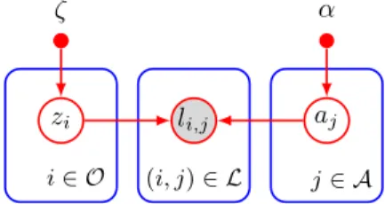
Figure 1 shows the trust model, in which large nodes represent random variables (RVs), and shaded nodes are ob-served; directed edges show the direction of causal influence; larger rectangles collect groups of RVs; and smaller nodes are the prior parameters of the model. Together, this represents a joint probability distribution. Ground-truths zi, labels lij,
and annotator reliability estimates, aj, are represented in the model by RVs. For simplicity, we focus on binary labels, i.e. zi, lij ∈ {0,1}, but this model can be used with
1-of-K categorical, ordinal, real scalar and real vector labels. Here, reliability estimates aj = (aj,0, aj,1), whereaj,0 andaj,1 are
annotator j’s true negative rate (specificity) and true positive rate (sensitivity) respectively.
i∈ O zi (i, j)∈ L li,j j∈ A aj ζ α
Fig. 1. Simple graphical model to infer ground truth from semi-trusted labels – objecti∈ Ohas hidden ground-truthzi, annotatorj∈ Ahas reliabilityaj, andlij∈ Lare observed labels. Parametersζandαencode prior knowledge.
A. Information Entropy and Gain
Information entropy and gain are used in Section III to anticipate the value of a new label. Information theory [22] tells us that before we know the outcome of some discrete random variable (RV), X, then its entropy is given by
H(X) = X
x∈AX
P(x) log2
1
P(x) (1)
1Similar to the model used in [2], where poor labellers are blacklisted.
whereAXare possible values forX, andP(x)is the probabil-ityX =x. Put simply,H(X)measures how much information we gain by knowing the outcome ofX.
For two RVs, X andY, the average entropy remaining in
X after knowingY is given by the conditional entropy
H(X|Y) = X
x,y∈AX×AY
P(x, y) log2 1
P(x|y) (2) whereP(x, y)is the joint probability that X=xandY =y, andP(x|y)is the probability X =xgivenY =y.
A related concept is mutual information, which measures the average reduction in entropy of X by knowingY, and is
I(X;Y) =H(X)−H(X|Y) (3) We define two more information theoretic quantities. First, the joint entropy of N independent RVsX1, . . . , XN is
H(X1, . . . , XN) = X
n
H(Xn) (4)
where independence means P(x1, x2. . . , xN) =QnP(xn).
If RVX has distributionP, and we think it has distribution
Q, then the Kullback-Leibler (KL) divergence measures the information we gain by learning true distribution P, and is
DKL(P||Q) = X x∈AX P(x) ln P(x) Q(x) (5)
Bayesian probabilistic models allow us to treat beliefs about unknown quantities as probability distributions over RVs. Together with the above information theoretic quantities, this concept allows us to measure how changing beliefs corre-spond to information gains. In the next section, we show how these measures can be used to guide knowledge acquisition.
III. ACTIVELABELCOLLECTION
This paper considers labels about objective reality, e.g. map locations; or about a shared view, e.g. whether a cycle route is challenging. Given this, the object being labelled must be expe-rienced. We categorise labels as either singular experienceor repeatable experience.Singular experiencelabels can only be acquired contemporaneously with the data, because the original experience cannot be sufficiently reconstructed from the data to be re-experienced. For example, the categorisation of human movement, e.g. cycling or walking, from accelerometer and gyroscope readings.Repeatable experiencelabels are such that a human inspecting or experiencing the data can reasonably be expected to label it. A trivial example is labelling an image based on its content. However, other examples exist, such as deciding whether there is traffic noise or human conversation in a sound recording (applicable to [17] and [5] respectively); or tagging the name and function of a map location (used in [5], [7], [8]). One common form ofrepeatable experiencelabelling is the up-/down-voting of data (or meta-data), e.g. suggested cycle routes [17], or the location of pot-holes [14]. This paper focuses on labels corresponding to repeatable experience, as the modelling techniques we employ require multiple labels for data items. More precisely, they require a degree of overlap in data items labelled by different annotators.
A. Object versus Annotator Centricity
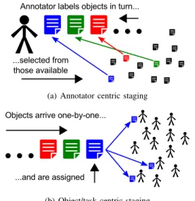
Crowdsourcing (and hence crowdsensing) annotation appli-cations come in many forms, and with different ways in which data items (more generally tasks) are selected for annotators, and how annotators are notified of requests, called staging. Figure 2 shows two common approaches. The first is anno-tator centric staging, see Figure 2(a), where annoanno-tators are central to the task assignment, and objects are selected, either individually or in batches, and queued for each annotator. This approach is common for the labelling of large data-sets, where annotators may attendsessionsof annotation. Inobject centric staging, see Figure 2(b), tasks arrive–or are selected in turn– and are then assigned to a waiting crowd of annotators. This approach is suited to live, on-going annotation, such as you might find in crowdsensing applications, where annotators are on callto answer questions for certain periods of the day.
(a) Annotator centric staging
(b) Object/task centric staging Fig. 2. Annotator centric versus object/task centric staging.
There are a number of additional concerns that can apply to both approaches, e.g. it may be that:
• Ground-truth corresponds to objective reality, or to hypo-thetical consensus, i.e. population majority view.
• The ground-truth is used as training inputs to learning algorithms, either for a single known algorithm or as a general purpose data-set.
• There is marginal utility to improving the confidence in ground-truth predictions beyond a threshold.
• QoI is either associated with the number of objects above the confidence threshold, or more generally with overall confidencemeasured across all objects.
• Some objects require higher confidence than others. This paper focuses on general purpose active labelling for objective ground-truth, treats all objects as equal in terms of information quality, and explores methods to improve both confidence threshold andoverall confidencemetrics. As stated in [1], there is no fundamental difference in the treatment of objective ground-truth and hypothetical consensus, so we approach both label types in the same way.
B. Object Centric Staging
Object centric labelling involves finding the right annota-tors for a given object or task. For this, the central authority must be able to request labels from individuals. There are a
number of additional concerns associated with object centric approaches. For example, the central authority may wish to:
• select one annotator for each object, or more than one.
• account for annotators failing to respond to requests, for annotators to respond at different rates, or with response rates that change with time
• limit the number of responses per object a priori by number, or reactively based on information measures.
• associate a higher cost with labels from some annotators, or with waiting longer for a response.
We focus on assigning one annotator per object at a time, assume that all annotators respond reasonably quickly, and allow costs to be a balance between time and number of la-bels. Other complicating factors are considered straightforward extensions of the methods here. We explore object centric approaches first and propose two generalstaging algorithms.
Buffered Streaming: A small number of objects/tasks are queued in a buffer. Iteratively, the queue’s head is assessed, and if the inference is still unsatisfactory, it is paired with an annotator and marked awaiting; otherwise the object is done (qualified). When a an awaiting label is returned (or times out), the object is moved to to the back of the queue.
Algorithm 1 Buffered Streaming.
Require: Buffer sizeb, qualification threshold,η
# Initialise buffer and pending & qualified objects B ← ∅, P ← ∅, Q ← ∅
whileO\Q 6=∅do while|B|+|P|< bdo
i←next object()
P ← P ∪ {i}
for alllabelslijreturned, with(i, j)∈ B)do # Store label, move object from buffer to pending L ← L ∪ {lij}, B ← B\{(i, j)}, P ← P ∪ {i} run learning(L)
for alli∈ Pdo ifqualifies(i, η)then
Q ← Q ∪ {i} else
j←pair annotator(i,A\BA) B ← B ∪ {(i, j)}. P ← P\{i} returnL
Buffered Pool Sampling: Objects are kept together in a pool, then sampled individually from the pool, either randomly or based on inference. Sampled objects are allocated to a annotator, and pushed to a finite awaiting buffer. Objects exit the awaiting buffer when response is received (or times out). As new responses become available, inference can be rerun, and satisfactory objects marked asqualified.
Algorithm 2 Buffered Pool Sampling.
Require: Buffer sizeb, qualification threshold,η
# Initialise buffer and qualified objects B ← ∅, Q ← ∅
whileO\Q 6=∅do while|B|< bdo
i←select object(O\(BO∪ Q)) j←pair annotator(i,A\BA) B ← B ∪ {(i, j)}
for alllabelslijreturned, with(i, j)∈ B)do # Store label, remove object from buffer L ← L ∪ {lij}, B ← B\{(i, j)} run learning(L)
Q ←all qualified(η)
returnL
Buffered streamingandbuffered pool samplingare outlined in Algorithms 1 and 2 respectively. In both algorithms, the set Ais the current set of annotators on call, and annotators
may dynamically join and leave this set. The set O contains all objects recognised by the system. In general, new ob-jects will be added to (or possibly removed from) this set with time. Busy annotators are defined as those in a buffer
BA def
={j|(i, j)∈ B}, and objects that have been assigned and are awaiting responses are defined as BO
def
={i|(i, j)∈ B}. next object() is used by buffered streaming to schedule the next object for labelling. Most simply, this is done by time-stamp or sampled at random. However, active-learning could be used when coupled with a classification/regression al-gorithm, see Section V. run learning(L) takes the current labelsL, and runs the inference, giving new ground-truth and reliability estimates. qualifies(i, η)determines if the inference for object i is sufficiently certain, and takes a threshold,
η, as argument – we discuss this further in Section III-D. all qualified(η)simply returns the set of all sufficiently certain objects, i.e. {i∈ O|qualifies(i, η)}.pair annotator(i,A\BA) predicts the best available annotator to label object i, and select object( ¯O)is used by buffered pool sampling to schedule the next object, both are discussed further in Section III-D. Buffered streaming is clearly more constrained than buffered pool sampling, the latter allowing the central authority to choose objects for every pairing based on changing need but with an additional overhead. However, buffered streaming ensures that each object qualifies in turn, and so can be used to rapidly acquire individual objects of a given quality. C. Annotator Centric Staging
Annotator centric labelling involves choosing appropriate objects for users who annotate in sessions. Annotator centric approaches may additionally wish to:
• allow annotators to terminate sessions at any point.
• have many annotators in sessionat any time.
• account for annotators working more or less quickly, with response times that depend on time and task.
We propose one annotator centric staging algorithm, which supports multiple annotators, who may join or terminate ses-sions freely. We assume response times are probabilistic but, for simplicity, assume these do not depend on task, time or annotator. Suitable extensions are straightforward.
Session Queues: Eachin sessionannotator is assigned a queue of up to n objects. At each iteration, annotators are assessed individually and suitable objects are allocated to return queues to size n. As annotators leave sessions, queues are cleared, and are freshly filled to sizen when they rejoin.
Algorithm 3 Session Queues.
Require: Queue sizec, qualification threshold,η
# Initialise session annotators, buffer and qualified objects
¯ A ← ∅, B ← ∅, Q ← ∅ whileO\Q 6=∅do for allj∈ A\A¯do Cj← ∅ ¯ A ← A, B ← {(i, j)|i∈ Cj, j∈A}¯ forj∈order annotators( ¯A)do
while|Cj|< cdo i←pair object(j,O\(BO∪ Q)) B ← B ∪ {(i, j)} L ←update labels() run learning(L) Q ←all qualified(η) returnL
Session Queuesstaging is outlined in Algorithm 3, where in-sessionannotators are denotedA¯, and update labels()adds
all newly returned labels to L. Finally, order annotators( ¯A) determines what order the in session annotators will have their queues filled, and pair object(j,O\(BO ∪ Q)) predicts the best unqueued object for annotator j to label, again, both are discussed further in Section III-D.
D. Information and Pairing Metrics
As discussed in Section II, the information content of probabilistic beliefs (or rather the degree of uncertainty) can be measured using the entropy of the corresponding random variable (RV). Here we show how this relates to the simple trust model from Section II for binary labels2, and how we use this to mark objects assatisfiedandpairthem with annotators. Recall that for labelsL, the trust model infers ground-truthzi
for each object i. For our binary model, zi∈ {0,1}, and this
unknown outcome is modelled by a RV,Zi, where
P(zi=z|L) = (1−µi)(1−z)µzi (6)
For notational simplicity, we drop the explicit label condi-tion, i.e.P(zi|L) =P(zi). Given this represents a probability
distribution over possible ground-truthszi, we can measure the entropy of Zi, using Equations (1) and (6), to give
H(Zi) =−(1−µi) log(1−µi)−µilog(µi) (7)
Each label lij we have not yet collected also represents a RVLij. We can again calculate the entropyH(Lij), by noting
P(lij =l) =X
z
P(lij =l|zi =z)P(zi=z) and
P(lij =l|zi =z) =aj,lI[l=z](1−aj,l)(1−I[l=z]) (8) whereI[.]is the indicator function.
From Equation (4), the total entropy over all objects is
H(O) =X
i∈O
H(Zi) (9)
because conditioned on theµis the Zis are independent. Information theory states that new data will on average add information [22], and hence decrease this entropy. Our aim is to select a new label lij that will most reduceH(O).
In our model, Lij has a more direct relationship to Zi, than other Zi0s, therefore we assume that choosing i and j to
maximally reduce H(Zi) is a good substitute strategy. This is not a formal argument. We present three pairing metrics,
P Mi,j, that predict the information gain inZi givenlij. Mutual Information (MI): If we knew no more about
Zi and Lij, than their joint probability, then the mutual information between Zi and Lij tells us how much new
information about Zi is acquired when we know lij. From Equations (2) and (3), this is
P Mi,j=I(Lij;Zi) =H(Lij)− X zi,lij∈{0,1} P(lij|zi)P(zi) log( 1 P(lij|zi) )
and can be evaluated using Equations (6), (7) and (8). Note that Lij and Zi are non-trivially coupled by the
inference model, so this may not be a perfectly accurate measure. However, it is a good first order approximation.
Information Gain (IG): Alternatively, we can predict how estimates of zi change, if we acquire lij. Define Zi0 as new probability distribution that would be inferred if lij were added to L. More specifically, if lij =l thenZi0 =Zi|lij=l. The information gained by addinglij =lis then estimated by
DKL(Zi|lij=l||Zi)3. As we do not know the label in advance, we calculate the expected information gain
P Mi,j=E(DKL(Zi0||Zi)|lij) =X
lij∈{0,1}
P(lij)DKL(Zi|lij||Zi)
= X
zi,lij∈{0,1}
P(lij|zi)P(zi)DKL(Zi|lij||Zi)
using Equations (6) and (8) and run learning(L ∪ {lij}). Thresholding (T): The third pairing metric, requires a thresholdη, and is the probability thatlij will increase object i’s entropy beyond thresholdη, e.g.P(H(Zi0)> η). This again usesrun learning(L ∪ {lij})and is given by
P(H(Zi0)> η) = X
lij∈{0,1}
P(lij)I[H(Zi|lij)> η]
Approximating Zi0: Note that information gain and thresholding’s use of run learning(L ∪ {lij}) can be expen-sive. However, methods from [1] and [2] use expectation-maximisation algorithms which iteratively approximate all µi
and aj simultaneously. For models already trained on
mod-erately sized label sets, adding one label and retraining is relatively cheap, and the vast majority of the change in Zi
occurs in the first E-step. For these reasons, we use a single E-step approximation of each Zi0, in our experiments. E. Selection, Qualification and Pairing
The above measures are used as follows:
select object( ¯O): in buffered pool sampling, schedules the next object given those available,O¯. This selection can take advantage of the entropy of ground-truth predictions, and we examine three possibilities: random, object chosen at random; most certain, choose objecti?= argmax
i∈O¯H(Zi); andleast
certain, choose objecti?= argmin
i∈O¯H(Zi).
qualifies(i, η): determines if the inference for objectiis sufficiently certain given scalar thresholdη >0. For generality, this uses the entropy as a measure of certainty, i.e. returning
H(Zi)≤η. For binary labels, this is equivalent to a probability
thresholdη0, where sufficient certainty corresponds toµi≤η0
or µi≥(1−η0); asymmetric thresholds are also possible.
pair object(j,O¯): finds the best objecti?, for annotator
j from those available. This uses any pairing metric, P M.,j, and returns i?= argmaxi∈O¯P Mi,j.
pair annotator(i,A¯): finds the best annotator, j?, for
objectifrom those available, again based on a pairing metric,
P Mi., wherej?= argmax
i∈A¯P Mi,j.
order annotators( ¯A): orders annotators for processing bysession queues. We explore three possibilities: Egality (E), i.e. random order; Meritocracy (M), i.e. by decreasing relia-bility; and Cannon Fodder (C), i.e. by increasing reliability.
3To see why, note thatZ
i|lij=lwould then be our best approximation of
the ground-truth.
pair annotator(., .)andpair object(., .), also support ran-dom (passive) pairing. However, the staging methods discussed here are only truly effective, with non-passive (active) pairing.
IV. RESULTS
The data-set most closely satisfying our experimental re-quirements was the Cub200 birds [2]. However, this has too little overlap between annotators, and no ground-truth. To ad-dress this, we trained the inference model on real labels for an individual binary Cub200 attribute, e.g. has size::small, then sampled500 object ground-truths and50annotator expertises from the inferred values, to synthetically generate labels with known ground-truth. Response times were sampled from an exponential distribution with mean of 1 minute.
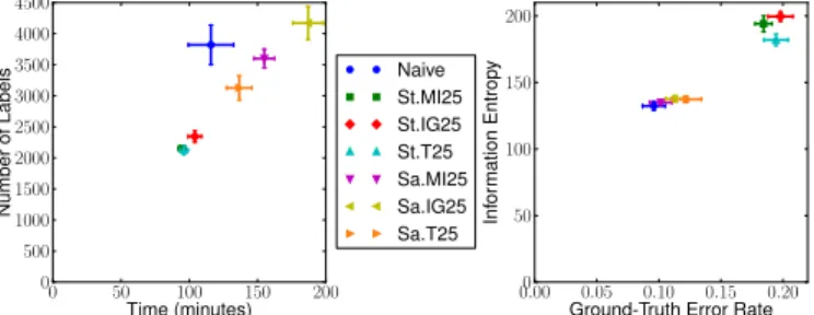
Figure 3(a) shows final label count, time, information entropy and ground-truth error rate for 5 runs of each object centric approach, as well as naive label collection. . Results show buffered streaming terminates more quickly than naive sampling and with just over half as many labels, while the best pool sampling method takes ∼ 50% longer, but again with fewer labels. Note that performance for all methods have error rates slightly higher than their thresholds, with buffered streaming as least accurate. Figure 3(b) shows how error rate threshold affects buffered streaming performance, with stricter thresholds reducing the number of labels (cost), but with increased time penalty. Mutual information pairing leads to fewest labels, while Thresholding gives the best accuracy.
(a) Streaming (St.) and pool sampling (Sa.); threshold error rate0.1.
(b) Buffered streaming, variable threshold error shown in legend. Fig. 3. Object centric results, with pairing metrics mutual information (MI), information gain (IG) and threshold crossing (T). Buffer size was25for active methods. Naive (N) method also shown. Error bars are 1 std. error.
Figure 4 (a) and (b) show the effects of varying ordering and queue length on the session queues staging respectively, where annotators join/leave sessions with probability0.1each iteration. Each experiment represents 5runs for a fixed50000 iterations, so only accuracy and entropy results are shown. Figure 4 (a), shows Egality ordering, with thresholding and information gain metrics, leads to higher accuracy than all
other choices. Figure 4 (b) uses Egality ordering and shows that larger queues give slightly higher throughput of labels.
N
(a) Annotator order (b) Session Queues
Fig. 4. Session queues, with pairing metrics: Mutual Information (MI), Thresholding (T) and Information Gain (IG). (a) compares (E)gality, (M)eritocracy, and (C)annon Fodder ordering, and (b) compares different Queue lengthsn, denoted Qn. Error bars are 1 std. error.
V. CONCLUSION
This paper outlines a family of approaches for active labelling within crowdsensing systems. These methods are based on information theoretic principles and cater for a variety of constraints on how labels are collected, i.e.staging. Object centric staging offers ways in which the number of labels required can be significantly reduced with small or no impact on time, and this will be particularly relevant when there is a cost associated with label collection. However, there are additional benefits, including a finer grained control over label collection, and cleaner data-sets, e.g. a smaller number of low quality labels. Unsurprisingly the naive approach is competitive on time though, as it allows maximal through-put of information, every annotator providing labels at their maximum rate. Annotator centric staging shows a marked improvement in accuracy over naive approaches for fixed label collection time, and labels can be queued in advance for each annotator. Both staging approaches can improve the acquisition rate and accuracy of inferred ground truth.
Aggressively optimising label acquisition could, in theory, lead to reduced accuracy due toconfirmation bias, i.e. seeking to confirm what one already believes. However, there was no evidence of this in our results. The entropy measure correlates well with the error rate for all of our algorithms.
In future work, we intend to support other label types & QoI measures (e.g. those in [23]); to account for time, task & annotator dependent response rates, and easier & harder tasks; and perform case studies on real collection in the wild. Another research avenue is to account for the specific learning algorithms that use the data, by integratingactive label collectionwithactive learning. The general principles outlined here offer a strategic base from which to explore these ideas.
ACKNOWLEDGMENT
This work was funded by EIT ICT Labs under the City Crowd Source Activity (13064). We are also grateful to Dr. Anil Bharath at Imperial, and to colleagues within the project, for the many useful discussions which influenced this work.
REFERENCES
[1] V. C. Raykar, S. Yu, L. H. Zhao, A. Jerebko, C. Florin, G. H. Valadez, L. Bogoni, and L. Moy, “Supervised Learning from Multiple Experts: Whom to Trust when Everyone Lies a Bit,” inICML, 2009, pp. 889– 896.
[2] P. Welinder and P. Perona, “Online crowdsourcing: rating annotators and obtaining cost-effective labels,” inCVPR, 2010, pp. 2262–2269. [3] D. Mendez and M. A. Labrador, “On Sensor Data Verification for
Participatory Sensing Sys.”J. of Networks, vol. 8, pp. 576–87, 2013. [4] M. Riahi, T. G. Papaioannou, I. Trummer, and K. Aberer, “Utility-driven
data acquisition in participatory sensing,” inProc. of 16th Intl. Conf. on Extending Database Technology, ser. EDBT ’13, 2013, pp. 251–262. [5] E. Miluzzo, N. D. Lane, K. Fodor, R. Peterson, H. Lu, M. Musolesi,
S. B. Eisenman, X. Zheng, and A. T. Campbell, “Sensing meets mobile social networks: the design, implementation and evaluation of the cenceme application,” inProc. of 6th ACM Conf. on Embedded Network Sensor Sys., 2008, pp. 337–50.
[6] A. Stopczynski, J. Larsen, S. Lehmann, L. Dynowski, and M. Fuentes, “Participatory bluetooth sensing: A method for acquiring spatio-temporal data about participant mobility and interactions at large scale events,” inPervasive Computing and Comms. Wksps. (PERCOM), 2013. [7] C. S. Karjalainen, “Moves: Activity Tracking without Gadgets,” 2013,
accessed on: 23/10/2013. [Online]. Available: moves-app.com [8] N. Bulusu, C. T. Chou, S. Kanhere, Y. Dong, S. Sehgal, D. Sullivan,
and L. Blazeski, “Participatory Sensing in Commerce: Using Mobile Camera Phones to Track Market Price Dispersion,” inWksp. on Urban, Community, and Social Apps. of Networked Sensing Sys., 2008. [9] L. Deng and L. P. Cox, “Livecompare: grocery bargain hunting through
participatory sensing,” inProc. of 10th Wksp. on Mobile Computing Sys. and Applications, 2009, pp. 4:1–4:6.
[10] S. Devarakonda, P. Sevusu, H. Liu, R. Liu, L. Iftode, and B. Nath, “Real-time air quality monitoring through mobile sensing in metropolitan areas,” inProc. of 2nd ACM SIGKDD Intl. Wksp. on Urban Computing, ser. UrbComp ’13, 2013, pp. 15:1–15:8.
[11] E. D’Hondt, M. Stevens, and A. Jacobs, “Participatory noise mapping works! an evaluation of participatory sensing as an alternative to stan-dard techniques for environmental monitoring,”Pervasive and Mobile Computing, vol. 9, no. 5, pp. 681 – 694, 2013.
[12] K. Han, E. A. Graham, D. Vassallo, and D. Estrin, “Enhancing mo-tivation in a mobile participatory sensing project through gaming,” in
SocialCom/PASSAT, 2011, pp. 1443–1448.
[13] J. Burke, D. Estrin, M. Hansen, A. Parker, N. Ramanathan, S. Reddy, and M. B. Srivastava, “Participatory Sensing,” in Wksp. on World-Sensor-Web, 2006, pp. 117–134.
[14] J. Eriksson, L. Girod, B. Hull, R. Newton, S. Madden, and H. Balakr-ishnan, “The Pothole Patrol: Using a Mobile Sensor Network for Road Surface Monitoring,” inMobile Sys., Apps. and Services, 2008. [15] U. Lee, B. Zhou, M. Gerla, E. Magistretti, P. Bellavista, and A. Corradi,
“Mobeyes: smart mobs for urban monitoring with a vehicular sensor network,”Wireless Comms., IEEE, vol. 13, no. 5, pp. 52–57, 2006. [16] W. Sha, D. Kwak, B. Nath, and L. Iftode, “Social vehicle navigation:
integrating shared driving experience into vehicle navigation,” inProc. of 14th Wksp. on Mobile Computing Sys. and Apps., 2013, pp. 16:1–6. [17] S. Reddy, K. Shilton, G. Denisov, C. Cenizal, D. Estrin, and M. Srivas-tava, “Biketastic: sensing and mapping for better biking,” inSIGCHI Conf. on Human Factors in Computing Sys., 2010, pp. 1817–1820. [18] E. A. Ni and C. X. Ling, “Active learning with c-certainty,” inProc.
of 16th Pacific-Asia Conf. on Advs. in Knowledge Discovery and Data Mining, 2012, pp. 231–242.
[19] P. Welinder, S. Branson, S. Belongie, and P. Perona, “The multidimen-sional wisdom of crowds,” inNIPS, 2010, pp. 2424–2432.
[20] J. Whitehill, P. Ruvolo, T. Wu, J. Bergsma, and J. Movellan, “Whose vote should count more: Optimal integration of labels from labelers of unknown expertise,” inNIPS, 2009, pp. 2035–2043.
[21] X. Liu, L. Li, and N. Memon, “A lightweight combinatorial approach for inferring the ground truth from multiple annotators,” inMach. Learn. and Data Mining in Pattern Recog., 2013, vol. 7988, pp. 616–628. [22] D. J. C. MacKay,Information Theory, Inference & Learning Algorithms.
New York, NY, USA: Cambridge University Press, 2004.
[23] C. Liu, P. Hui, J. Branch, and B. Yang, “Qoi-aware energy manage-ment for wireless sensor networks,” in Pervasive Comp. and Coms. Workshops (PERCOM Workshops), 2011, pp. 8–13.