Ex post analysis of economic impacts from wind power development in U.S. counties

University of Nebraska - Lincoln

University of Nebraska - Lincoln

DigitalCommons@University of Nebraska - Lincoln

DigitalCommons@University of Nebraska - Lincoln

Publications from USDA-ARS / UNL Faculty

U.S. Department of Agriculture: Agricultural

_{Research Service, Lincoln, Nebraska}

2012

Ex post analysis of economic impacts from wind power

Ex post analysis of economic impacts from wind power

development in U.S. counties

development in U.S. counties

Jason P. Brown

USDA, [email protected]

John Pender

USDA,, [email protected]

Ryan Wiser

Lawrence Berkeley National Laboratory, [email protected]

Eric Lantz

National Renewable Energy Laboratory, [email protected]

Ben Hoen

Lawrence Berkeley National Laboratory, [email protected]

Follow this and additional works at:

https://digitalcommons.unl.edu/usdaarsfacpub

Brown, Jason P.; Pender, John; Wiser, Ryan; Lantz, Eric; and Hoen, Ben, "Ex post analysis of economic

impacts from wind power development in U.S. counties" (2012). Publications from USDA-ARS / UNL

Faculty. 1144.

https://digitalcommons.unl.edu/usdaarsfacpub/1144

This Article is brought to you for free and open access by the U.S. Department of Agriculture: Agricultural Research

Service, Lincoln, Nebraska at DigitalCommons@University of Nebraska - Lincoln. It has been accepted for inclusion in

Publications from USDA-ARS / UNL Faculty by an authorized administrator of DigitalCommons@University of

Nebraska - Lincoln.

Ex post analysis of economic impacts from wind power development in

U.S. counties

☆

Jason P. Brown

⁎

, John Pender

, Ryan Wiser

, Eric Lantz

, Ben Hoen

a

USDA, Economic Research Service, 355 E St. SW, Washington, D.C. 20024, United States b_{Lawrence Berkeley National Laboratory, 1 Cyclotron Road, Berkeley, CA 94720, United States} c

National Renewable Energy Laboratory, 1617 Cole Boulevard, Golden, CO 80401, United States d

Lawrence Berkeley National Laboratory, 20 Sawmill Road, Milan, NY 1257, United States

a b s t r a c t

a r t i c l e i n f o

Article history:

Received 16 December 2011 Received in revised form 3 July 2012 Accepted 7 July 2012

Available online 20 July 2012

JEL classification:

Q20 Q42 R11 Keywords: Wind power Economic development Ex post analysis

Wind power development has surged in recent years in the United States. Policymakers and economic devel-opment practitioners to date have typically relied upon project-level case studies or modeled input–output estimates to assess the economic development impacts from wind power, often focusing on potential local, state-wide, or national employment or earnings impacts. Building on this literature, we conduct an ex post econometric analysis of the county-level economic development impacts of wind power installations from 2000 through 2008 in a large, wind-rich region in the country. Taking into account factors influencing wind turbine location, wefind an aggregate increase in county-level personal income and employment of ap-proximately $11,000 and 0.5 jobs per megawatt of wind power capacity installed over the sample period of 2000 to 2008. These estimates appear broadly consistent with modeled input–output results, and translate to a median increase in total county personal income and employment of 0.2% and 0.4% for counties with installed wind power over the same period.

Published by Elsevier B.V.

1. Introduction

Wind power development has expanded rapidly in the United States (Wiser and Bolinger, 2011). Though annual capacity additions vary from year-to-year, cumulative installations totaled roughly 47 giga-watts (GW) by the end of 2011. From 2007 through 2010, wind contrib-uted 36% of all new electric generation capacity added to the U.S. power system. Worldwide, the USA is second only to China in annual additions and cumulative capacity (Wiser and Bolinger, 2011).

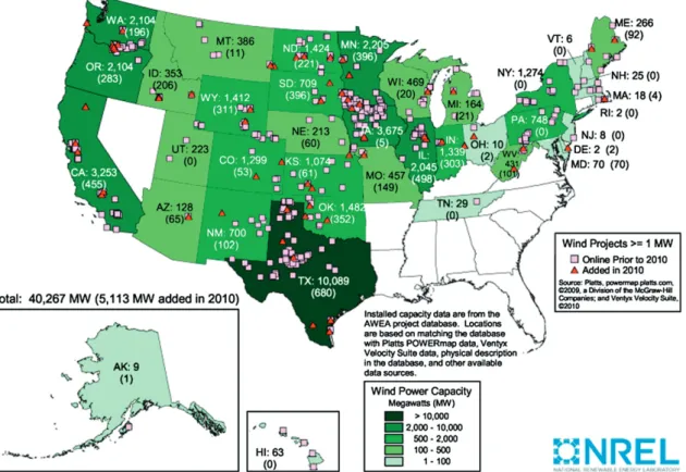
Utility-scale wind power installations have been developed throughout the nation, with the notable exception of portions of the Southeast, which lacks a high-quality on-shore wind resource. Higher quality wind resources and favorable policies have led to some con-centration of wind development in the Great Plains, but installations are also substantial on the Pacific seaboard and in the Northeast (Fig. 1). Wind power installed by the end of 2010 has been estimated

to be capable of delivering more than 5% of total electricity genera-tion in 13 states, with four states exceeding 10% (South Dakota, Iowa, North Dakota, and Minnesota). In aggregate, wind power installed through 2010 was capable of generating more than 2.5% of the nation's electricity supply (Wiser and Bolinger, 2011). With con-tinued and accelerated growth, studies have shown that it is techni-cally feasible for 20% of the U.S. electric supply to be derived from wind power by 2030 (e.g.,U.S. DOE, 2008).

Though the improving economics of wind energy has played a major role in driving development over the past decades (Bolinger and Wiser, 2009; Wiser et al., 2011), government policy has also been important in supporting growth. At the federal level, production-based tax credits (PTC) have helped reduce the cost of wind energy to purchasers (Lu et al., 2011), while the more recent ability to convert the PTC to an up-front cash grant has helped the wind industry weather thefinancial crisis (Bolinger et al., 2010). At the state level, a combination of policies, such as Renewables Portfolio Standards (RPS) andfinancial incentives, have been important (Bird et al., 2005). Most recently, however, RPS policies that impose an obligation on electricity suppliers to use a certain amount of renewable energy in their supply mix have been the domi-nant state policy tool (Wiser and Barbose, 2008). Oftenly noted motivat-ing factors behind policy support include wind energy's potential global, regional, and local environmental benefits such as net carbon reduction when used in place of traditional fossil fuels (i.e., coal or natural gas); presumed fuel diversity bene_fits; and the potential impact of wind ☆ The views expressed here are those of the authors, and may not be attributed to the

U.S. Department of Agriculture, the Economic Research Service, the Lawrence Berkeley National Laboratory, the U.S. Department of Energy, or the National Renewable Energy Laboratory. NBNL's and NREL's contribution to this work was funded by the U.S. DOE (Wind & Water Power Program) under Contract No. DE-AC02-05CH11231.

⁎Corresponding author.

E-mail addresses:[email protected](J.P. Brown),[email protected] (J. Pender),[email protected](R. Wiser),[email protected](E. Lantz),[email protected] (B. Hoen).

0140-9883/$–see front matter. Published by Elsevier B.V. doi:10.1016/j.eneco.2012.07.010

Contents lists available atSciVerse ScienceDirect

Energy Economics

j o u r n a l h o m e p a g e : w w w . e l s e v i e r . c o m / l o c a t e / e n e c o

power installations on local, state, and/or national employment and economic development.

Despite the role of economic development potential in driving wind energy policy, questions persist with respect to the existence, magni-tude, distribution, and durability of the employment and economic development impacts associated with renewable energy. Such debates are largely focused on national level impacts in the USA and abroad, and often relate to the treatment of“gross”vs.“net”effects. For exam-ple, in addition to the potentially positive direct employment and eco-nomic development impacts of renewable energy development and equipment manufacturing, are employment and economic losses asso-ciated with the displacement of other energy sources or land uses con-sidered? Additionally, what are the macroeconomic effects (i.e., costs vs. benefits) of policy support for renewable energy, for example, over-all impacts to electricity rates (e.g.,Frondel et al., 2010; Hillebrand et al., 2006; Lehr et al., 2008; Sathaye et al., 2011)? Regardless of these larger debates about gross and net impacts that often play out on a national stage, however, the possibility of contributing tolocaleconomic devel-opment is particularly salient in rural areas, where wind power plants are often constructed and where new investment, earnings growth, and employment opportunities have otherwise often been trending downward for some time.

This work applies ex post econometric evaluation methods using county-level data, and covering multiple wind power projects, to explore the impact of wind power development on personal income and employment in U.S. counties. The analysis is not intended to inform the debate over state or national“net”effects. Nor does the analysis presented here seek to provide a comprehensive benefit–cost analysis of wind energy–such an analysis would need to investigate the myriad of potential costs and benefits of wind energy development, and is be-yond the scope of this paper. Instead, this paper provides an empirical assessment of county-level economic development impacts while

avoiding many of the potential weaknesses apparent in other methods that have been used to assess such local impacts (seeSection 2). In ad-dition, it creates the opportunity to test the validity of previous input–

output modeling analyses by comparing the modeled estimates already available in the literature with those derived here based on anex-post

econometric analysis of the local impact of actual wind power develop-ment. To our knowledge, this effort represents afirst of its kind applica-tion of these methods to the study of the local economic impacts from wind power development.⁎

The balance of the paper is organized as follows:Section 2reviews the literature on measuring the economic development impacts from wind power, with a focus on local effects, and notes the general short-comings typically associated with the methodologies used to date; Section 3presents the methods and data used in this study;Section 4 describes the study region and sample data;Section 5 contains the results of the study, including the findings of multiple alternative econometric models; andSection 6provides a summary of conclusions and a brief discussion of future research directions.

2. Measuring the local economic impacts of wind power development

Wind power development can affect the local economies in which projects are situated in many ways, including but not necessarily limited to:

1. Wind power development directly affects the employment and in-come of those working in the industry, particularly during the con-struction phase of a project, but also during the operations phase. Source: Wiser and Bolinger(2011)

Numbers within states represent cumulative installed wind capacity and, in parentheses, annual additions in 2010.

Fig. 1.Location of wind power development in the United States. Note: Numbers within states represent cumulative installed wind capacity and, in parentheses, annual additions in 2010. Source:Wiser and Bolinger (2011).

⁎_{A number of studies have used econometric analysis to test for larger,country level} relationships between, for example, renewable energy and economic growth and other variables (e.g.,Chien and Hu, 2008; Menegaki, 2011).

2. Wind power construction and operations expenditures may gener-ate indirect demand for goods and services (e.g., gravel, concrete, vehicles, fuel, hardware, and consumables) produced or sold by other industries in the local economy, contributing to increased employment and income in those industries.

3. If wind turbines are absentee-owned, lease payments by project owners to local landowners contribute to local income. However, if wind turbines displace other uses of land or other resources, the net impact of these payments on the local economy could be less than the gross amount of the payments. For example, wind turbines may reduce agricultural production due to their footprint which would reduce income from farming. According to one study, wind turbines permanently displace on average 0.74 acres of land per MW and temporarily 1.74 acres per MW of installed capacity (Denholm et al., 2009). The fact that the land owners voluntarily accept payments for the wind development suggests that their net benefits exceed the net costs.

4. If wind turbines are locally-owned, the profits that owners earn add to the income of community residents. However, this effect depends on the opportunity costs of these investments (as well as the level of the profits earned), which can result in negative income impacts.

5. Property taxes or payments in lieu of property taxes paid by wind energy operators can contribute to increased local government revenues.

6. Spending on goods and services in the local economy by local res-idents and governments from these additional sources of income as well as by workers involved in construction or operations activ-ities can induce further local economic impacts.

7. Wind power development may positively or negatively affect the desire of people to live, visit or work in the community, in turn af-fecting migration and commuting_flows and income from tourism as well as demand for land, with subsequent potential impacts on property values, property tax revenues, and other aspects of the local economy.

8. Wind power development in one community may affect employ-ment and income of people in nearby communities through vari-ous means, such as by inducing increased demand for goods and services from nearby communities, or by affecting commuting or migration to or from these communities. Changes in economic ac-tivity in nearby communities can in turn affect economic acac-tivity in the counties where the wind power development is occurring.

Given the multiple pathways of impact, assessing the local eco-nomic development impacts of wind power installations is likely to require multiple methods and outcome measures. However, to date almost all studies of the economic development impacts of wind power have relied on two methods: (1) project-level case studies of the gross impacts of actual wind power plants (e.g., GAO, 2004; Pedden, 2006) which are, in effect, an assessment of the direct im-pacts of these plants based on employment, cost, and revenue data from particular project developers or operators; and (2) input–output model estimates of the potential direct, indirect, and induced impacts of an individual planned (or completed) wind power plant or an ag-gregate amount of assumed wind development activity (e.g.,GAO, 2004; Lantz and Tegen, 2008, 2009; Reategui and Hendrickson, 2011; Reategui and Tegen, 2008; U.S. DOE, 2008).

These methods have produced a wide range of estimated impacts of wind power development in the United States across a variety of studies and contexts. Although much of the publicly available literature focuses on state or regional impacts (e.g., Lantz and Tegen, 2009; Pedden, 2006; Reategui and Hendrickson, 2011; Reategui and Tegen, 2008), a limited number of studies have emphasized local areas or counties (e.g.,DanMar and Associates, 1996; ECONorthwest, 2002; GAO, 2004; Kildegaard and Myers-Kuykindall, 2006; NEA, 2003; Slattery et al., 2011; Torgerson et al., 2006).

Focusing on employment, impacts estimated from previous research to local regions or counties (including direct, indirect and induced im-pacts as derived from input_–output models) from absentee-owned wind power plants (i.e., projects owned by non-local businesses or indi-viduals) have been estimated to range from approximately 0.1 to 2.6 jobs per MW of installed capacity during the construction period (DanMar and Associates, 1996; ECONorthwest, 2002; GAO, 2004; NEA, 2003; Slattery et al., 2011), and from 0.1 to 0.6 jobs/MW during the op-erations period (DanMar and Associates, 1996; ECONorthwest, 2002; GAO, 2004; Kildegaard and Myers-Kuykindall, 2006; NEA, 2003; Slattery et al., 2011; Torgerson et al., 2006). The estimated employment impacts of locally-owned plants (again including direct, indirect, and induced impacts) during the construction period are similar to those es-timated for absentee-owned plants. Alternatively, during the opera-tions period, estimated locally-owned plant impacts are notably larger than absentee-owned estimated impacts, ranging from 0.5 to 1.3 jobs/ MW, as a result of the indirect and induced impacts accruing from the estimated returns to local investors (DanMar and Associates, 1996; GAO, 2004; Kildegaard, 2010; Kildegaard and Myers-Kuykindall, 2006; Torgerson et al., 2006).

Focusing on labor income, previous research that has estimated impacts during the long-term operations period by this same set of input–output analyses have found impacts range from about $5,000/ MW to $18,000/MW (in 2010 $) for the more-common absentee-owned plants (DanMar and Associates, 1996; ECONorthwest, 2002; GAO, 2004; NEA, 2003; Slattery et al., 2011; Torgerson et al., 2006), and from $18,000/MW to $43,000/MW for the far-less-common locally-owned plants (DanMar and Associates, 1996; GAO, 2004; Kildegaard, 2010; Kildegaard and Myers-Kuykindall, 2006; Torgerson et al., 2006). Additionally, some of these studies have examined impacts on total eco-nomic output (GAO, 2004). During the operating phase, total ecoeco-nomic output impacts have been estimated to range from $13,000/MW to $55,000/MW for absentee-owned plants (DanMar and Associates, 1996; GAO, 2004; Slattery et al., 2011; Torgerson et al., 2006) and from $82,000/MW to $140,000/MW for locally-owned plants (DanMar and Associates, 1996; GAO, 2004; Torgerson et al., 2006).

Estimates derived from input–output modeling and project-level case studies, however, are subject to several well known criticisms. Both approaches, when applied at a local level, typically focus on project-specific gross impacts and may not reflect the full net impact resulting from a given project or set of projects. For example, local eco-nomic development losses associated with the possible displacement of other local energy sources or with increased electricity rates due to wind development are often not considered. Similarly, displacement of other land uses or of other uses of the local capital and labor required to construct and operate wind power projects are not considered in such analyses. Though these simplifications are more problematic when conducting state or national analyses than when conducting county-level assessments, they may nonetheless fail to provide a com-plete picture of the county-wide impact from a given project or set of projects.

Additionally, project-level case studies might further be questioned because they are often based on self-reported direct employment and income, which may differ from the actual direct employment and come resulting from project operations, particularly when there is an in-centive to boost the favorable impression of a project (e.g.,Loveridge, 2004). Moreover, by focusing on direct impacts (and often ignoring in-direct and induced effects), case studies of actual projects may under-state the economic development impacts of wind development. There may also be questions about whether the individual case studies are representative, and whether these studies report results consistently (e.g., peak jobs versus average jobs versus full-time equivalents).

With regard to input–output models, a variety of assumptions are required that may be questioned, and there is some evidence from empirical studies outside of the wind sector that the estimated contri-bution of industrial development to local economic growth can be

overstated, because of assumptions normally adhered to with the models (e.g.,Edmiston, 2004; Fox and Murray, 2004; Kilkenny and Partridge, 2009). Input_–output models assume that all industrial inputs and factors of production are used infixed proportions and that the sup-ply of these inputs and factors responds perfectly elastically to increases in demand with no increase in prices or costs of production. Such as-sumptions may not be too problematic where the additional source of demand is a small proportion of the local economy, or when the econo-my is relatively open and integrated with outside economies, ensuring that the local supply of factors of production are highly elastic.†In the case of wind power development in isolated rural areas, however, this assumption may not always be reasonable, creating the possibility of upwardly biased estimates of positive local impacts.

Another issue related to input–output model assumptions is that the model coefficients are sometimes based on national input–output tables, adapted to the local economy based on local industrial compo-sition. The high level of resulting disaggregation available in some off-the-shelf modeling packages can create a false sense of precision, with the model re_flecting inter-industrial linkages for sectors that may not exist or that exist at a different level or in different form than predicted by national industrial composition data (Loveridge, 2004). Such models are thus better at predicting impacts in hypothet-ical communities that have the characteristics reflected in the model rather than predicting impacts in actual communities, unless consid-erable effort is made to calibrate the model to local conditions. Fur-thermore, the parameters in off-the-shelf models may not be well adapted to the particular requirements of a small new sector, such as wind power generation.

Efforts have been made to overcome these limitations to input–

output models by better tailoring their data specifically for the sectors under analysis and adjusting the local purchase coefficients to more rea-sonably re_flect the available local supply of goods and services for a given project. For example, the National Renewable Energy Laboratory (NREL) has taken these issues into consideration in its development of the Jobs and Economic Development Impacts (JEDI) Wind model (NREL, 2008), used by (among others)Lantz and Tegen (2008)to per-form a sensitivity analysis of wind-power-related economic develop-ment drivers and the economic developdevelop-ment benefits from wind. Even when using a modified input–output approach, however, questions may remain on the extent to which the modifications are sufficiently tailored to account for the simplifications inherent in input–output models.

A third limitation of traditional input–output models is that they ac-count only for industry linkages, but do not acac-count for the inter-actions between_firms and other important actors in the economy, such as households and governments (Loveridge, 2004). For example, profits earned by local owners of wind projects, lease payments by absentee-owners, and property tax payments are important contributors to the local economic impacts of wind power development, but these pay-ments would not be incorporated into a traditional input–output model. One way to address such issues is to use a social accounting ma-trix (SAM), which builds upon the input–output approach. A SAM uses information from input–output tables, but also accounts for other mon-etaryflows within an economy (Round, 2003; Thorbecke, 1998). For ex-ample, the model used byLantz and Tegen (2008)is based on a SAM for local economies, enabling analysis of the impacts of local ownership of wind power plants, lease payments and property taxes. More recently, Allan et al. (2011)used a SAM to investigate the implications of local revenue sharing from wind development in the Shetland Islands. Nev-ertheless, because they are based on input–output models, even SAM models may still have many of the same limitations as more traditional input–output models, such as the assumptions that all inputs are used

infixed proportions to output and that input supplies are perfectly elas-tic (Loveridge, 2004; Round, 2003).

Input_–output and SAM modeling approaches also generally predict positive indirect and induced impacts of new sources of demand (i.e., they imply that economic multipliers are greater than 1). However, if one considers the possible displacement effects and opportunity costs associated with pursuing such new demands, it becomes clear that the net impacts of investing in a new opportunity are not necessarily positive. For example, if wind power development displaced other uses of local land, labor or capital that would yield a higher return than wind power, the net effect could be to reduce rather than increase local income. Addi-tionally, if wind power development reduced the attractiveness of living in a particular community (e.g., due to negative perceptions of its visual impact, noise, or other impacts), this could potentially have negative im-pacts on local property values and the ability to attract and retain com-munity residents. While the likelihood of such events is unknown, it should be noted that such effects are not addressed by standard input–

output and SAM modeling approaches.

Finally, the potential for spatial feedback of development in near-by economies is also not typically captured near-by these approaches.‡In a regional input–output or SAM model, income spent outside of the re-gion of study is generally treated as entirely lost to the local economy. However, if income increases in nearby regions as a result of wind power development in the region of study (due to the same kind of direct, indirect and induced impacts that occur within the region), this increase in income may induce increased demand for goods and services supplied by people and businesses in the region being stud-ied. Thus, not all of the income thatflows out of the region will nec-essarily be lost.

Many of the limitations of both model-based estimates and project-level case studies can be addressed by analyzing the ex post impacts of past developments using econometric methods. Impacts measured by the econometric approach need not apply the many as-sumptions required by input–output models and can be based on a large and representative set of actual wind power plants. Since both the local economic costs and benefits of wind power development are likely to be reflected in measured changes in outcomes such as employment and personal income, econometric estimation can also directly account for any substitution and displacement effects that occur within the local economy and provide a better reflection of the net impacts of this development within a given study area. Relat-ed to this, because direct and indirect effects, as well as impacts on property values, migration and commutingflows, are also likely to be reflected in the measured changes in outcomes, the econometric approach allows for a more complete set of possible impacts to be considered.

3. Empirical model and estimation

We use an ex post econometric approach relying on publicly avail-able data to estimate the county-level economic impacts of wind pro-ject installations. We focus on wind power development from 2000 through 2008 in the large, wind-rich Great Plains region of the USA, as discussed in more depth later. Though we are not able to address all of the issues raised in the previous section (for example, we do not directly investigate impacts of wind power development on prop-erty values, tourism, migration, or commutingflows), our approach builds on the existing literature by avoiding many of the potential weaknesses apparent in other methods. We focus our investigation

†_{This will not be the case forfixed factors of production, such as land. However, as} noted above, wind projects generally do not displace much land use if located in agri-culturalfields or with other land uses that are not significantly disrupted.

‡_{Traditional approaches have not accounted for spatial spillovers but there are} re-gional methodologies that now allow one to capture these effects to some extent. To date, however, these regional methods have not been used in analyzing wind power development impacts.

on two of the more prevalent economic development outcomes em-phasized in this literature: personal income§_{and employment.}

Speci_fically, the change in per capita annual personal income and employment at the county level are used as the economic outcomes of interest. Changes in these outcome variables over time are hypoth-esized to be affected by a county's socio-economic and demographic characteristics, and by the amount of wind power development in that county. Given that we observe geographic clusters of counties with wind power installations (see Fig. 4), it is also hypothesized that changes in the outcome variables could be impacted by wind power development in neighboring counties. Given these hypothe-sizes, we therefore assume that changes in annual per capita personal income and employment (y) at the county level are impacted by the counties' own socio-economic and demographic characteristics (X), the counties' own wind power development (D) (measured in mega-watts of capacity per capita), neighboring counties' wind power development (WD), and state-levelfixed effects (S), as shown by:

y¼Z Xð ;DÞβþWDγþαSþμ; ð1Þ

whereZis vector containingXandD,Wis an (n×n) spatial weight ma-trix containing information about county neighbors, andμis a vector of residuals. Neighborhood criteria are often based on distance or commonly shared borders between spatial units, with the elements in

Wtypically being row-standardized so that each row sums to one (Anselin, 2002). For the purpose of the present study, queen order-one contiguity was selected for the neighboring criteria.¶

The location of wind power development (D) may be endogenous to the outcome variables of interest. This could be because a change in per capita income or employment in a county impacts wind development (e.g., if increased income enables local investors to invest in wind devel-opment), or because wind development is impacted by unobserved fac-tors that also affect the change in per capita income or employment (e.g., if wind development is more likely to take place in communities that have fewer alternative economic opportunities or less ability to in-vest in such opportunities due to unobserved factors such as the quality of local resources or local leadership or entrepreneurial capacity). In such a case, estimation using methods such as ordinary least squares (OLS) can result in biased estimates. For example, if communities with fewer alternative economic opportunities are more likely to invest in wind power, then communities with more wind power installed could tend to have lower rates of growth than other communities, biasing downward an OLS-estimated economic impact of wind power.

A common approach for dealing with endogenous regressors is in-strumental variables (IV) estimation. Availability of a high quality wind resource (i.e., high-speed wind) is likely a primary factor affecting the location and amount of wind power development and is unlikely to be directly related to the outcome measures in question (change in in-come per capita and employment from 2000 to 2008).⁎⁎Among other

factors, available capacity on existing nearby transmission lines, de-mand for new power generation, state and local policy drivers, and cit-ing and permittcit-ing processes are also likely to be important in wind project development. Constructing convincing instrumental variables based on these latter factors, however, is challenging if not impossible. Consistent data on available transmission capacity, for example, are not available, and datasets similarly do not exist that fully characterize federal, state and local citing and permitting processes and demand for new power generation. Consequently, to instrument actual wind power development we ultimately use two instrumental variables re-lated to wind resource conditions: (1) the presence of wind resource potential across power classes 3–7 in a county (where 3 is towards the low end of feasible power classes for economic wind energy devel-opment and 7 represents areas with the highest wind speeds), and (2) the cumulative technical potential for wind power development in a county, measured in megawatts, based on the amount of class 3_–7 winds available.,†† ‡‡

Standard tests were used to determine the strength, validity and necessity of using the instrumental variables (IV) model compared to a more efficient (but possibly inconsistent) single-stage model such as an OLS model. These include tests for weak instruments, over-identification, and exogeneity of the presumed endogenous re-gressors. The weak instrument test investigates whether the instru-ments are sufficiently correlated with the endogenous variable to avoid large biases.§§The over-identification test investigates the hy-pothesis that the instrumental variables are valid (i.e., exogenous–

not correlated with the error term in the model–and valid to exclude from the main equation being estimated). The exogeneity test investi-gates whether the potentially endogenous regressors are exogenous (a rejection implies that they are not). Rejection of this last hypothesis (together with passing thefirst two tests for the validity of the IV model) supports the IV model as the best model, while failure to reject supports the use of the more efficient single stage model (Wooldridge, 2002, pp. 483–486).

4. Data and sample description

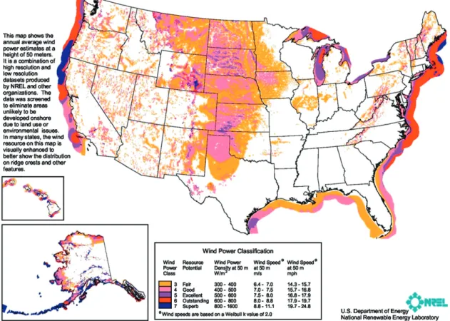
The prevalence of wind varies greatly across the USA.Fig. 2shows a U.S. wind resource map developed by the National Renewable Ener-gy Laboratory (NREL). As illustrated, the 12 states in the Great Plains and the eastern edge of the Rocky Mountains have some of the highest on-shore wind resource potential (i.e., classes 3 to 7 wind re-source regimes). Therefore, it follows that these states are also the lo-cation of substantial wind power capacity, as of the end of 2010, as was depicted in Fig. 1. This region was selected for the present

§

We also decomposed county personal income into its various components and estimat-ed the models on wages/salary and rental income separately. Such an approach could allow one to separate the impact of wind power development on lease payments from other im-pacts on personal income, which includes both. Though the full statistical model results from this analysis are not presented here, as one would expect, the effect sizes were found to be smaller than when personal income is used, but were not statistically significant.

¶

Our results were indifferent to other specifications ofW, such ask-nearest neigh-bor and inverse distance criterion.

⁎⁎_{It could be that high winds reduce economic activity in a county (separately from their} impact on wind energy development) by making such counties less attractive places to live and work. It seems unlikely that any effect of high winds on the attractiveness of a commu-nity would change substantially over a relatively short period of time such as between 2000 and 2008. Thus, although theabsolutelevel of economic activity in a county in any given year may be affected by the average amount of wind in that county,changesin economic activity over the period may not be much affected (i.e., this could be afixed effect in econo-metric terms). In that case, the fact that we are investigating changes in income and em-ployment rather than levels of income and emem-ployment helps to reduce concern about this possible source of bias. Our statistical test of the over-identification restrictions (test discussed and reported later) further supports our argument that these are valid instru-ments that can be excluded from the primary regression.

††_{County-level wind potential data were provided by NREL. The indicator variable took} the value of one if the county had any wind potential across the power classes 3–7. The other instrument was the level of aggregate wind potential (in MW terms) summed across the power classes for each county. Wind resource estimates were derived from NREL's validated wind resource maps at 50 m height where available (seehttp://www. windpoweringamerica.gov), and supplemented with other high resolution state wind maps or low resolution data from the Wind Energy Resource Atlas of the United States (Elliott et. al., 1986). Wind resource data werefiltered to eliminate areas that are consid-ered unsuitable or unlikely for development due to environmental or land use reasons (e.g., national parks and other protected federal, state, and private land as well as urban, wetland and water areas, and slopes in excess of 20%). Potential wind generation capacity is based on an assumed wind project land-use power density of 5 MW/km2

, a standard in-dustry rule of thumb (Denholm et al., 2009).

‡‡_{We also attempted to use distance to the nearest transmission line based upon GIS} calculations, but the variables constructed in this fashion were found to be weak in-struments. Regardless, they were not correlated with either outcome variable, suggesting little risk of omitted variable bias as a result of proximity to transmission lines.

§§_{Bound, et al. (1995)proved that, with weak instruments, the coefficients of an}

instru-mental variables (IV) estimation can be more biased with afinite sample than the coeffi -cients from a comparable ordinary least squares (OLS) estimation, even though the IV model is asymptotically consistent and the OLS model is not (if the assumptions of the IV model hold). Standard tests for weak instruments are discussed inWooldridge (2002).

analysis because, in part, of this potential and development, and also because the region of states is contiguous and is relatively homoge-nous in its socio-economic and demographic characteristics. The use of a more homogenous, contiguous region is anticipated to reduce the impacts of omitted variables on the econometric analysis, and grouping states based on economic and social factors is common (e.g., the Bureau of Economic Analysis has grouped states into“BEA Regions” for similar reasons; historically, the guiding principle for the grouping of states into regions was homogeneity with regard to economic and social factors (Kort, 2008)). As a result, the 12 states in-cluded in the present analysis include: Iowa, Kansas, Minnesota, Ne-braska, North Dakota, South Dakota, New Mexico, Oklahoma, Texas, Colorado, Montana, and Wyoming, representing 1009 counties.¶¶

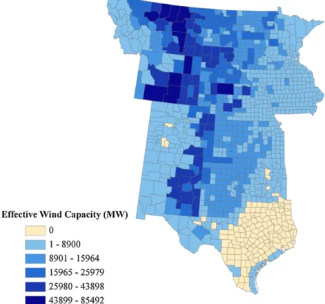
Data on installed wind power capacity by county and year compiled by the Lawrence Berkeley National Laboratory (LBNL) were obtained for the period of 2000 through 2008. NREL provided county-level wind re-source potential data for the USA for wind classes 3 through 7, data that were used to construct appropriate instrumental variables for actual wind capacity additions.Fig. 3shows the total technical resource poten-tial for wind power capacity (measured in megawatts, MW) summed across all of the relevant wind power classes (3 to 7) for each county in the study region. The counties with highest wind potential are clus-tered in parts of Wyoming, Montana, North and South Dakota, as well as in the eastern edge of Colorado and New Mexico.Fig. 4shows the amount of actual wind power capacity installed in the counties in the study region over the period from 2000 to 2008. The counties in the study region with the highest installed wind power capacity over the study period are located in north-central/west Texas, southern Minne-sota, and northern Iowa.Fig. 4also indicates that counties with wind

power installations tend to neighbor counties that also have installed wind power.

Table 1provides summary statistics of the data used to model the county-level economic impacts of wind turbine development, which–

with the exception of the key explanatory variable of interest and the two outcome variables–were taken from the year 2000 or prior. The key explanatory variable of interest,mwcap, is a per capita measure of the total (i.e., cumulative) amount of wind power capacity (in MW) installed in a county over the study period of 2000–2008 (in other words, it represents the change in installed capacity between 2000 and 2008). The key outcome measures are the county-level change in annual per capita income and per capita employment over the same time period. Though wind power projects may have economic develop-ment impacts at the county level during both the operations and con-struction phases, our analysis does not seek to separately analyze these two effects. However, because our outcome measures are the change in per capita income and employment from 2000 to 2008, while the key explanatory variablemwcapmeasures the (per capita) quantity of wind capacity installed over the period of 2000–2008, the results of the present analysis should be dominated by operating period impacts.⁎⁎⁎

Previous studies that have modeled changes in county-level per capita income and employment were utilized to determine what kinds of socioeconomic, demographic, and other control variables to include in our analysis. Indicators of initial (2000 or before) outcomes

¶¶

The analysis was also conducted on the entire U.S. lower 48 states. The results were quantitatively similar. Results are available from the authors upon request.

⁎⁎⁎_{Because the construction of a wind project normally lasts no longer than one year,} only those wind power projects constructed in 2008 can logically have construction period impacts that are captured in the present analysis. Further, projects constructed from 2000–2007 will only show operation period impacts, because construction im-pacts largely would have faded. Though, because of a lack of precision in the available data, we did not attempt to disentangle these two types of impacts.

Source: National Renewable Energy Laboratory

Fig. 3.Technical resource potential for wind capacity (Power Class 3–7, MW).

in per capita income (pci) are usually used to account for growth tra-jectories over the study period that may differ depending on pre-study-period income levels (e.g.,Isserman and Rephann, 1995; Pender and Reeder, 2011; Stenberg, et al., 2009). The determinants of economic demand are also commonly used, such as the level of population (pop) and the poverty rate (poverty) (Deller et al., 2001). Recent research on economic growth in very rural places such as the Great Plains region has concluded that two major factors affecting rural growth are remoteness to cities and natural amenities (Deller et al., 2001; Partridge et al., 2008; Wu and Gopinath, 2008). Distances to urban population centers of 25,000, 100,000, 250,000, 500,000 and 1,000,000 were calculated for each county using GIS methods.††† Since the literature is unclear on what specific natural amenities mat-ter the most (McGranahan et al., 2011), a natural amenities scale was selected for the present analysis (USDA ERS, 2004).

Urban agglomeration economies have also been shown to impact changes in per capita income, in particular where urban and rural areas are interdependent (Castle et al., 2011). Urban agglomeration is measured using population density (popdens) and an indicator of whether a county is part of a metropolitan area (metro). Economic structure as it relates to regional specialization has also been shown to be of importance (Kim, 1998). For example, as industrial sectors rise and fall it has implications for per capita economic development in a county depending upon its industrial composition. We control for this by using the share of employment in major industries such as ag-riculture, forestry,fishing, and hunting (agffh), construction (const), manufacturing (manuf), and the retail trade sector (retrade). Land use as part of the economic structure is accounted for by the share of farm land to total area in a county (farmland).

Consistent with modern economic growth theory, as the stock of human capital increases in a county, income has been shown to grow (Rupasingha et al., 2002). Human capital is measured using ed-ucational attainment via the percentage of the adult population with associate (pedas), bachelors (pedbs), and masters (pedms) degrees. Labor accessibility and participation have also been shown to contrib-ute to economic growth in a region (Partridge and Rickman, 2003). Here they are measured using a county's unemployment rate (uer) and the share of adult men (wfullmsh) and women (wfullwsh) work-ing full time in 1999.

†††_{Using these distance measures also introduces a possible concern about multicollinearity,} since a town that is far from a small city is also far from a larger city. However, the maximum variance inflation factor for these measures was 2.6, indicating that multicollinearity was not a major problem. Another concern is that Euclidean distance is not a perfect indicator of ac-cess to urban areas, considering topographic characteristics and differences in acac-cess to high-ways. Other urban access measures were considered including drive time and incremental distance measures. The results were similar in direction, size, and significance.

Table 1

Descriptive statistics.

Variable Label Mean Std. dev.

Change in per capita income 2000–20081

($/capita) dpci 11,593 5488

Change in per capita employment 2000–20081

(jobs/capita) demp 0.050 0.056

Change in installed wind capacity 2000–2008 (MW/capita) mwcap 0.003 0.022 Technical wind resource potential (power class 3–7, MW) twrp 8042.33 9422.48

Per capita income ($)1 _{pci 23,640 5370}

Population (thous.)1

pop 45.20 166.08

Poverty rate (%)2

poverty 13.43 5.98

Natural amenity scale3

nascale 3.45 1.13

Agriculture, forestry,fishing, & hunting share of employment1

agffh 0.11 0.09

Construction share of employment1

const 0.07 0.02

Manufacturing share of employment1

manuf 0.11 0.07

Retail & trade share of employment1 _{retrade 0.11 0.02} Adult population (25 yrs >) with associates degree (%)2

pedas 6.05 2.07

Adult population (25 yrs >) with bachelors degree (%)2

pedbs 12.23 4.60

Adult population (25 yrs. >) with masters degree (%)2

pedms 3.48 1.88

Population density (persons per square mile)2

popdens 57.75 221.03

Amount of Interstate highway (miles)4

interst 12.44 22.31

Distance to nearest urban population of 25,000(miles)5 _{d25k 43.53 38.95} Distance to nearest urban population of 100,000 (miles)5 _{d100k 93.38 75.25} Distance to nearest urban population of 250,000 (miles)5

d250k 154.00 109.86

Distance to nearest urban population of 500,000 (miles)5

d500k 238.80 165.68

Distance to nearest urban population of 1,000,000 (miles)5

d1000k 402.80 243.21

Unemployment rate (%)6

uer 3.83 1.56

Farmland share of total acres7

farmland 0.42 0.28

Population weighted distance to highway on-ramp (km)5 _{hwyaccess 45.60 43.02}

Rural population share2 _{rurpopsh 0.65 0.31}

Farmer population share2

frmpopsh 0.09 0.08

African American population share2

afrpopsh 0.02 0.05

Child population share2

chdpopsh 0.26 0.03

Elderly population share2

eldpopsh 0.16 0.05

Share of adult men working full time2

wfullmsh 0.65 0.06

Share of adult women working full time2 _{wfullwsh 0.42 0.05}

Metro county (yes/no)8 _{metro 0.20 0.40}

Notes: N= 1009; Source:

1

Bureau of Economic Analysis, REIS;

2

Census Bureau, 2000 Census;

3 _{Economic Research Service;} 4 _{US DOT;}

5

ERS GIS team calculations;

6

Bureau of Labor Statistics;

7

Census Bureau, U.S. Counties;

8

Differences in county demographics that might impact consumption ability (Deller et al., 2001) are controlled for by the rural population share (rurpopsh), the farming population share (frmpopsh), African American population share (afrpopsh), children population share (chdpopsh), and the elderly population share (eldpopsh).

Infrastructure has also been shown to positively impact county eco-nomic growth (Monchuk et al., 2007). Infrastructure is controlled for by using miles of Interstate highway within the county (interst) and the population weighted mean distance to a highway on-ramp (hwyaccess). Statefixed effects were also included in the model (though not shown inTable 1) to control for differences in unobserved state poli-cies or conditions that might impact changes in per capita county in-come and employment.‡‡‡

5. Results

We present three sets of models used to estimate the impact of wind power plant installation (MW per capita) on,first, changes in income per capita (Table 2) and, secondly, employment per capita (Table 3) be-tween 2000 and 2008 using data for the 1009 counties in the sample re-gion. Thefirst set of columns inTable 2shows the personal income results from a simple linear model estimated by ordinary least squares (OLS).§§§_{The assumptions of this model are that per capita wind turbine} installation (mwcap) is exogenous and that local spatial spillovers from wind power development in neighboring counties are not present.¶¶¶ Overall the model explains approximately 38% of the variation in the change of annual per capita income. A keyfinding is that with each ad-ditional MW of wind power installed over the 2000–2008 period, the change in total annual personal income in the county from 2000 to 2008 increased by $9,326. Other factors that had a statistically signifi -cant association with income growth include the share of employment in agricultural, forestry,fishing, and hunting (agffh) and manufacturing (manuf), with less growth in per capita income associated with greater employment shares in these industries. Higher initial per capita income levels (pci) were correlated with larger changes in per capita income. Additionally, counties with longer distances to the nearest highway in-terchange (hwyaccess) or to urban population centers of half a million people (d500k), larger percentages of the adult population with an asso-ciate's degree (pedas), larger rural shares of the population (rurpopsh) and larger shares of men working full time (wfullmsh) were associated with greater growth in per capita income. Conversely, a larger percent-age of the adult population with a master's degree (pedms), child share of the population (chdpopsh) and a larger share of women working full time (wfullwsh) were associated with less change in per capita income. This likely reflects fewer economic opportunities for these segments of the population due to life cycle effects as well as the possibility of wage inequality between women and men. Metropolitan counties had small-er changes in psmall-er capita income, which suggests convsmall-ergence of income between metro and non-metropolitan counties.

The second set of columns inTable 2reports the IV results (without accounting for local spillovers). A Durbin–Wu–Hausman test (t-stat= 6.98, p-value= 0.000) confirmed the endogeneity ofmwcap. Addition-ally, the chosen instruments had sufficient strength and were valid according to the F-test and Hansen J-test. Combined, these results indi-cate the presence of bias in the OLS estimates. The IV coefficient on

mwcapshows that for every additional MW of installed wind power ca-pacity, total county personal income increased by $11,150 over the 2000 to 2008 period, a somewhat larger impact than estimated previ-ously with OLS.

To account for the possibility of local geographic spillovers from wind development in neighboring counties on income, the third set of columns inTable 2presents IV results when including both mwcap

andW × mwcap, assuming that both are endogenous. Spatial lags of the initial set of instruments were used to instrumentW × mwcap. The coef_ficient on W × mwcap, which re_flects local spillovers from wind power development, was not statistically significant. Although the di-rect personal income effects of in-county wind power development were statistically significant in this third regression, and somewhat larger in magnitude than found in the first two models, F-tests for weak instruments used formwcap(F= 2.72⁎⁎⁎, d.o.f. = 2 and 964) and W × mwcap(F= 11.77⁎⁎⁎, d.o.f. = 2 and 964) raise a concern about weak instrument bias when accounting for the number of endog-enous regressors (2) and instruments (4) (see Table 5.1 ofStock and Yogo, 2005). Because of this, and because this regression failed to show statistical evidence of local spillovers from wind power develop-ment, the IV model including only direct impacts from wind power de-velopment (the second column inTable 2) is preferred.

To aid in establishing the economic signi_ficance of wind power de-velopment, the estimated marginal effect of $11,150 per MW can be translated into a county-level total annual personal income measure by multiplying the marginal effect by the installed wind power capac-ity of each county that had installed wind power (assuming that the same marginal effect of wind power development would occur in all counties). Reporting the resulting number as a percentage of total county personal income levels in 2000 for those counties with installed capacity helps gauge wind power development's importance in driving economic activity on a historical basis. Among the counties in the sample that experienced wind development from 2000–2008, the resulting percentage increase in county-level personal income as a result of wind development equaled 0.03% at the 25th percentile of counties, 0.22% at the 50th percentile of counties, and 0.86% at the 75th percentile of counties. In absolute terms, the average estimated increase in annual personal income from wind power development for the top quartile of counties (in terms of percentage impact, i.e., 0.86% and above) was estimated to be $2,552,679 over the sample period.

Table 3shows the results from the models estimating net employ-ment impacts. Wind power developemploy-ment was not found to have a sta-tistically significant effect on per capita net employment in the OLS specification (thefirst set of columns), while factors significantly as-sociated with increases in employment per capita were higher levels of personal income (pci) and higher shares of adult men working full-time (wfullmsh). Conversely, covariates that were negatively cor-related with changes in county employment per capita were higher shares of employment in construction (const), manufacturing (manuf) and retail trade (retrade), higher shares of farmland ( farm-land), children (chdpopsh), and women working full-time (wfullwsh), and metropolitan counties (metro).

The IV results for per capita employment impacts were similar for most variables, with the exception of wind power capacity (mwcap), which was treated as endogenous in these regressions and was found to be statistically significant. For each additional MW of installed wind power capacity in a county over the 2000 to 2008 time period, 0.48 net additional jobs were added according to thefirst IV model, which does not consider the possibility of local spillovers from wind develop-ment in neighboring counties (second column ofTable 3). As with the personal income IV results, the strength and validity of the instrumental variables are supported by the F-test and Hansen's J test, and the endogeneity ofmwcapis supported by a Durbin–Wu–Hausman test (t-stat= 1.90, p-value = 0.057). The difference between the OLS and IV coefficients reflects the relative bias in the OLS estimate ofmwcap

when it is assumed to be exogenous. Regardless, we also note that the coefficient is only statistically significant at the 90% confidence level.

To account for the possibility of local geographic spillovers from wind development in neighboring counties, the second IV model ‡‡‡_{Wyoming serves as the omitted category in the regressions.}

§§§

Standard errors of the coefficients have been adjusted for heteroskedasticity.

¶¶¶_{The spatial lag of wind power development,W×mwcap, was not statistically significant}

in the OLS models, suggesting that local spillovers do not impact changes in per capita income or employment in a meaningful way. We revisited the presence of local spillovers as an en-dogenous regressor when considering the endogeneity ofmwcap; the results for this case are discussed further below.

includes bothmwcapandW × mwcapand treats both as endogenous (third column ofTable 3). The resulting coefficient formwcapshows a marginally statistically significant but somewhat smaller impact of wind power development on net county-level employment (0.37 jobs per MW). The same model shows a small and statistically insig-nificant impact of wind power development in neighboring counties. Similar to the income results, the F‐test of the instruments in the sec-ond IV model revealed a potential concern about weak instrument bias; hence thefirst IV model is preferred.

Using the results from thefirst IV model (0.48 jobs per MW), those counties in the sample that experienced wind development from 2000–2008 are estimated to have experienced a net increase in county-level employment from the base period in 2000 of 0.1%, 0.4%, and 1.4% at the 25th, 50th, and 75th percentiles of counties, re-spectively. In absolute terms, the average estimated number of net additional jobs from wind power development in the top quartile of counties (in terms of percentage impact, i.e., 1.4% and above) was es-timated to be 132 over the sample period.

These econometric results are not strictly comparable to the input–

output model estimates presented earlier because they: (1) emphasize the broader category of personal income rather than the narrower cat-egory of labor income (or the even-broader catcat-egory of total economic output), and (2) include construction period impacts for installations occurring in the year 2008. All else being equal, these factors would be expected to yield higher estimated impacts in the present analysis when compared to the input–output derived labor income and employ-ment results presented earlier. On the other hand, the results presented here are the estimated net effect of wind power development at the county level, which, all else being equal, should be lower than the

gross impacts reported earlier from input–output analyses. Notwith-standing these differences, the estimated impact on personal income and employment of approximately $11,000/MW and 0.5 jobs/MW in 2008 can be compared to the results from previous input–output models which, as reported earlier, range from $5000 to $18,000 per MW (for labor income) and 0.1 to 0.6 jobs per MW (for employment) in the operating phase of wind development for absentee-owned plants (the dominant case) (DanMar and Associates, 1996; GAO, 2004; NEA, 2003; Slattery et al., 2011; Torgerson et al., 2006).

6. Conclusions

Policymakers and economic development practitioners have recent-ly been looking to wind power development as a rural development strategy, though questions persist with respect to the existence, magni-tude, and durability of the potential impacts. Many analyses of such impacts have relied onex antemodeled estimates of the expected eco-nomic impacts of wind power development.

This study is thefirst that we are aware of to empirically test for the economic development impacts of wind power installations in U.S. counties using an ex post econometric approach. We applied this method to a large region of the country that hosts a large number of existing wind power projects, mainly in the Great Plains, to test the hypotheses that wind power installations increased county-level in-come and employment growth between 2000 and 2008. The analysis does not address questions concerning state or national“net”effects. Nor does the analysis seek to provide a comprehensive benefit–cost analysis of wind energy of the type that would be desired in making local, state, or national policy decisions– such an analysis would Table 2

Change in per capita income 2000–2008.

Variable OLS IV Estimation IV Estimation–Local spillovers

Coefficient Robust S.E. Coefficient Robust S.E. Coefficient Robust S.E. mwcap 9326.30⁎⁎ 4858.10 11,150.05⁎⁎ 5410.78 13,948.23⁎⁎ 6268.66 W × mwcap −10,593.58 11,614.18 pci 457.74⁎⁎⁎ 159.19 458.89⁎⁎⁎ 162.51 457.28⁎⁎⁎ 163.12 pop −2.05 1.27 −2.05 1.30 −2.06 1.30 poverty 3.65 105.96 6.69 108.20 8.69 108.56 nascale 150.71 131.31 151.06 134.11 158.51 134.15 agffh −17,346.00⁎⁎⁎ 6018.60 −17,383.61⁎⁎⁎ 6149.17 −17,573.79⁎⁎⁎ 6162.49 const −12,938.00 9232.60 −12,648.34 9432.33 −13,076.99 9606.09 manuf −24,799.00⁎⁎⁎ 2881.70 −24,740.39⁎⁎⁎ 2944.06 −25,007.41⁎⁎⁎ 2990.97 retrade −7169.80 9242.90 −7069.71 9440.70 −7627.98 9529.68 pedas 215.86⁎⁎ 95.44 215.64⁎⁎ 97.52 212.87⁎⁎ 97.80 pedbs −47.69 91.53 −48.18 93.47 −48.39 93.66 pedms −400.69⁎⁎⁎ 153.90 −399.62⁎⁎ 157.24 −410.88⁎⁎⁎ 158.31 popdens −0.09 0.92 −0.09 0.94 −0.10 0.94 metro −1467.80⁎⁎⁎ 366.43 −1458.50⁎⁎⁎ 374.42 −1458.54⁎⁎⁎ 374.28 uer 261.29 170.40 259.04 174.95 250.08 175.10 interst 10.22 8.54 10.20 8.73 10.00 8.72 farmland 1245.50 915.45 1254.78 935.34 1301.06 936.79 hwyaccess 10.25⁎ 5.49 10.28⁎ 5.61 10.22⁎ 5.62 d25k −3.74 4.51 −3.78 4.61 −3.94 4.61 d100k 3.14 3.20 3.15 3.27 3.08 3.28 d250k −1.89 2.57 −1.90 2.63 −1.82 2.63 d500k 3.21⁎⁎⁎ 1.13 3.24⁎⁎⁎ 1.16 3.26⁎⁎⁎ 1.16 d1,000k −0.35 0.71 −0.36 0.73 −0.39 0.73 rurpopsh 2206.10⁎⁎⁎ 828.51 2194.24⁎⁎⁎ 846.41 2133.58⁎⁎ 851.29 frmpopsh 10,340.00 6336.60 10,331.45 6469.94 10,264.92 6475.08 afrpopsh 2427.70 3134.50 2519.21 3200.89 2462.54 3216.80 chdpopsh −19,243.00⁎⁎ 8823.80 −19,247.39⁎⁎ 9013.07 −19,521.30⁎⁎ 9024.85 eldpopsh −3740.70 8182.10 −3592.00 8353.54 −3466.64 8358.86 wfullmsh 20,288.00⁎⁎⁎ 5134.90 20,409.65⁎⁎⁎ 5246.88 20,627.76⁎⁎⁎ 5249.64 wfullwsh −17,788.00⁎⁎⁎ 4961.00 −17810.95⁎⁎⁎ 5068.54 −17,796.97⁎⁎⁎ 5078.13 constant 6011.40 6330.20 5832.22 6464.29 6009.57 6496.73 Adj. R2 0.38 0.41 0.41 F-test (IVs) – 9.26⁎⁎⁎ 2.72⁎⁎⁎, 11.77⁎⁎⁎ Hansen J – 7.30 7.67

need to investigate the myriad potential costs and benefits of wind energy development. Instead, the present paper provides an empiri-cal assessment of netlocal economic development impacts, while avoiding many of the potential weaknesses of other methods that have been used to assess such local impacts.

Taking into account the endogeneity of location decisions of wind power development, wefind an average aggregate increase in annual personal income of approximately $11,000 per megawatt of wind power capacity installed over the sample period, and an average ag-gregate increase in net county-level employment of 0.5 jobs per megawatt. Thesefigures translate to a median increase in total county personal income and employment of 0.22% and 0.4%, respectively, for counties with installed wind power over the 2000 to 2008 period.

Overall, ourfindings suggest that empirical econometric methods are useful in measuring the ex post impacts of wind power develop-ment. Interestingly, despite a number of known limitations to the standard application of input–output models to estimating economic development impacts, our results are of a similar general magnitude to input–output derived estimated impacts. Though the two sets of results are not strictly comparable, this suggests that input–output models that are used to assess the economic impacts of wind energy (at least at the county or local level) may not be unduly impacted by the generic limitations to those models discussed earlier in this paper. Whether the local economic development impacts of wind power are sizable enough to be policy relevant on a local, state, or national level is open to debate. Regardless, more research on these impacts is warranted. First, questions about gross vs. net effects, especially when conducting analysis on a state, national or global scale, remain open. Second, with regard to local effects, further econometric analysis may

be warranted to try to separate construction and operation period im-pacts. Third, with additional wind power development (and therefore additional available data), it may be possible to extend the econometric approach to investigate other possible outcome variables, including the impact of wind power development on county-level migration, proper-ty values, and other variables of interest beyond personal income and employment. Fourth, and related, with more wind development it may also be possible to decompose income impacts into various constit-uent parts, for example impacts on wage vs. rental income. Finally, with more data, the analysis could also be extended to additional years and to more regions of the country, potentially teasing out the existence of and reasons for any temporal or locational variations in the economic development impacts of wind power installations.

References

Allan, G., McGregor, P., Swales, K., 2011. The importance of revenue sharing for the local economic impacts of a renewable energy project: a social accounting matrix approach. Reg. Stud. 45 (9), 1171–1186.

Anselin, L., 2002. Under the hood: issues in the specification and interpretation of spatial regression models. Agric. Econ. 17 (3), 247–267.

Bird, L., Bolinger, M., Gagliano, T., Wiser, R., Brown, M., Parsons, B., 2005. Policies and mar-ket factors driving wind power development in the United States. Energy Policy 33 (11), 1397–1407.

Bolinger, M., Wiser, R., 2009. Wind power price trends in the United States: struggling to remain competitive in the face of strong growth. Energy Policy 37 (3), 1061–1071. Bolinger, M., Wiser, R., Darghouth, N., 2010. Preliminary evaluation of the impact of the

Section 1603 Treasury grant program on renewable energy deployment in 2009. LBNL-3188E. Lawrence Berkeley National Laboratory, Berkeley, CA.

Bound, J., Jaeger, D.A., Baker, R.M., 1995. Problems with instrumental variables estima-tion when the correlaestima-tion between the instruments and the exogenous explanato-ry variable is weak. J. Am. Stat. Assoc. 90, 443–450.

Table 3

Change in per capita employment 2000–2008.

Variable OLS IV Estimation IV Estimation–local spillovers

Coefficient Robust S.E. Coefficient Robust S.E. Coefficient Robust S.E.

mwcap −0.0655 0.1000 0.4817⁎ 0.2812 0.3721⁎ 0.2253 W × mwcap 0.0835 0.2732 pci 0.0028⁎ 0.0016 0.0031⁎ 0.0016 0.0031⁎ 0.0016 pop −0.00002 0.00001 −0.00002 0.00001 −0.00002 0.00001 poverty −0.0001 0.0012 0.0008 0.0013 0.0006 0.0013 nascale 0.0009 0.0015 0.0010 0.0016 0.0010 0.0016 agffh −0.0989 0.0784 −0.1101 0.0819 −0.1068 0.0813 const −0.2971⁎⁎⁎ 0.1128 −0.2102⁎ 0.1183 −0.2207⁎ 0.1190 manuf −0.2200⁎⁎⁎ 0.0387 −0.2023⁎⁎⁎ 0.0403 −0.2031⁎⁎⁎ 0.0392 retrade −0.2195⁎ 0.1207 −0.1895 0.1237 −0.1899 0.1220 pedas −0.0006 0.0014 −0.0007 0.0015 −0.0006 0.0014 pedbs −0.0019 0.0014 −0.0021 0.0014 −0.0021 0.0014 pedms −0.0012 0.0033 −0.0009 0.0034 −0.0009 0.0034 popdens −0.00002 0.00001 −0.00002 0.00001 −0.00002 0.00001 metro −0.0181⁎⁎⁎ 0.0053 −0.0153⁎⁎⁎ 0.0054 −0.0156⁎⁎⁎ 0.0054 uer 0.0019 0.0023 0.0013 0.0026 0.0014 0.0025 interst 0.00002 0.0001 0.00001 0.0001 0.00001 0.0001 farmland −0.0363⁎⁎⁎ 0.0114 −0.0335⁎⁎⁎ 0.0119 −0.0343⁎⁎⁎ 0.0120 hwyaccess 0.00001 0.00006 0.00002 0.0001 0.00002 0.0001 d25k −0.00006 0.00005 −0.0001 0.0001 −0.0001 0.0001 d100k 0.00002 0.00004 0.00002 0.00004 0.00002 0.00004 d250k −0.00002 0.00003 −0.00002 0.00003 −0.00002 0.00003 d500k 0.00001 0.00001 0.00002 0.00001 0.00002 0.00001 d1,000k 0.000001 0.00001 −0.000003 0.00001 −0.000003 0.00001 rurpopsh 0.0047 0.0102 0.0011 0.0107 0.0022 0.0105 frmpopsh 0.0333 0.0675 0.0308 0.0778 0.0317 0.0752 afrpopsh −0.0561 0.0467 −0.0287 0.0475 −0.0326 0.0480 chdpopsh −0.2001⁎ 0.1183 −0.2015⁎ 0.1216 −0.1991 0.1227 eldpopsh 0.0413 0.0868 0.0859 0.0902 0.0778 0.0897 wfullmsh 0.2839⁎⁎⁎ 0.0778 0.3205⁎⁎⁎ 0.0849 0.3129⁎⁎⁎ 0.0834 wfullwsh −0.1262⁎ 0.0678 −0.1330⁎ 0.0712 −0.1321⁎ 0.0706 constant 0.0037 0.0808 −0.0500 0.0829 −0.0428 0.0820 Adj. R2 0.21 0.21 0.22 F-test (IVs) – 9.26⁎⁎⁎ 2.72⁎⁎⁎, 11.77⁎⁎⁎ Hansen J – 1.08 1.03