Center for Financial Studies
No. 2011/19
Default Risk in an Interconnected Banking
System with Endogeneous Asset Markets
Marcel Bluhm and Jan Pieter Krahnen
Center for Financial Studies Telefon: +49 (0)69 798-30050
Center for Financial Studies
The Center for Financial Studies is a nonprofit research organization, supported by an association of more than 120 banks, insurance companies, industrial corporations and public institutions. Established in 1968 and closely affiliated with the University of Frankfurt, it provides a strong link between the financial community and academia. The CFS Working Paper Series presents the result of scientific research on selected topics in the field of money, banking and finance. The authors were either participants in the Center´s Research Fellow Program or members of one of the Center´s Research Projects.
If you would like to know more about the Center for Financial Studies, please let us know of your interest.
* The authors are grateful to Peter Ockenfels as well as to participants of the 3rd Annual Conference of the Post-Graduate Programme on Global Financial Markets in Jena and the Research Conference on Financial Networks in Geneva in 2011 for valuable comments. 1 The Wang Yanan Institute for Studies in Economics at Xiamen University and Center for Financial Studies at Goethe University
CFS Working Paper No. 2011/19
Default Risk in an Interconnected Banking
System with Endogeneous Asset Markets*
Marcel Bluhm
1and Jan Pieter Krahnen
2August 2011
Abstract:
This paper analyzes the emergence of systemic risk in a network model of interconnected bank balance sheets. Given a shock to asset values of one or several banks, systemic risk in the form of multiple bank defaults depends on the strength of balance sheets and asset market liquidity. The price of bank assets on the secondary market is endogenous in the model, thereby relating funding liquidity to expected solvency - an important stylized fact of banking crises. Based on the concept of a system value at risk, Shapley values are used to define the systemic risk charge levied upon individual banks. Using a parallelized simulated annealing algorithm the properties of an optimal charge are derived. Among other things we find that there is not necessarily a correspondence between a bank's contribution to systemic risk - which determines its risk charge - and the capital that is optimally injected into it to make the financial system more resilient to systemic risk. The analysis has policy implications for the design of optimal bank levies.
JEL Classification: G01, G18, G33
Keywords: Systemic Risk, Systemic Risk Charge, Systemic Risk Fund, Macroprudential Supervision, Shapley Value, Financial Network
1 Introduction
In a manner unexpected only a few years ago, the global nancial crisis which started in 2007 has demonstrated that a system of interconnected nancial institutions may be subject to a systemic breakdown, with large eects on the real economy. In this paper a numerical model is used to analyze a network of nancial institutions subject to capital requirements. The model allows to replicate important stylized facts of systemic risk which emerged during the recent nancial crisis. We then introduce the concept of a Systemic Value at Risk (SVaR) which allows to simultaneously determine both, a fair risk charge as well as the optimal macro-prudential capital endowment, for nancial institutions in the system. Among other things we nd that there is not necessarily a correspondence between a bank's1 contribution to
systemic risk which determines its risk charge and the optimal capital injection which would render the nancial system more resilient with respect to systemic risk.
As there are many dierent sources of systemic risk, and also dierent potential consequences for the real economy, there is not a single denition of systemic risk.2 An early denition of systemic risk was given in Group
of Ten: Systemic nancial risk is the risk that an event will trigger a loss of economic value or condence in, and attendant increases is uncertainly about, a substantial portion of the nancial system that is serious enough to quite probably have signicant adverse eects on the real economy. Sys-temic risk events can be sudden and unexpected, or the likelihood of their occurrence can build up through time in the absence of appropriate policy responses. The adverse real economic eects from systemic problems are gen-erally seen arising from disruptions to the payment system, to credit ows, and from the destruction of asset values.3 Lo (2009) proposes analyzing
a set of risk measures to capture systemic risk in the entire nancial sys-tem. These risk measures capture the six dimensions `leverage', `liquidity', `correlation', `concentration', `sensitivities', and `connectedness'. The IMF denes systemic risk as large losses to other nancial institutions induced by the failure of a particular institution due to its interconnectedness4 and
the Financial Stability Board, International Monetary Fund, and Bank for International Settlements describe systemic risk in a report to the G-20 as a
1In the following the terms `banks' and `nancial institutions' will be used
interchange-ably.
2See paper 2 of International Monetary Fund (2009) for a comprehensive discussion of
dierent denitions of systemic risk.
3Group of Ten (2001), p. 126.
risk of disruption to nancial services that is (i) caused by an impairment of all or parts of the nancial system and (ii) has the potential to have serious negative consequences for the real economy.5 Following closely the latter
denition, in this paper we dene systemic risk as the danger that failures within the nancial system will mean that an adequate supply of credit and nancial services to the economy is no longer guaranteed, so that negative real eects will follow.
A main driver of the recent nancial crisis was the state of the nan-cial system.6 Large nancial institutions tended to be highly leveraged,
while their portfolio structures were relatively homogeneous, and returns were highly correlated.7 There were also close ties to the so-called shadow
banking sector, obscuring balance sheets and rendering the nancial system fragile. In the course of the crisis numerous institutions had to be bailed out because their insolvency would have put the nancial system at risk via triggering a cascade of other nancial institutions' defaults. The increase in systemic risk was essentially driven by three factors, the size of the nancial institutions, the direct links among these institutions, as well as the indirect, asset market-driven links.
First of all, the default of a nancial institution which is relatively large can put the nancial system at risk. For example, in line with our denition of systemic risk, one can expect that the insolvency of even a single large bank constitutes a serious threat to the nancial system and the real economy of the entire country. Switzerland is a good example, as its two global banks, UBS and Credit Suisse, pose a signicant risk for the country's nancial system and the wider economy because of their mere size. This is why banks like UBS or CS were called `too-big-to-fail' in the recent nancial crisis.
Second, banks that are highly interlinked with other nancial institutions can also threaten the nancial system through their network of exposures to other banks, domestically and abroad. If such a bank defaults on its liabilities it can directly induce losses on its creditor banks which on their part might spread the shock further in case they also default. For example, during the recent nancial crisis, the insurance company American International group (AIG) was bailed out because of its interlinkages, via CDS (Credit Default
5Financial Stability Board, International Monetary Fund, and Bank for International
Settlements (2009), p. 2.
6For a general overview on the causes and consequences of the recent nancial crisis
see, inter alia, Issing, Asmussen, Krahnen, Regling, Weidmann, and White (2009), Borio (2008), Brunnermeier (2009), and Gorton (2010a).
7For an analysis of the role of the shadow banking system in the recent nancial
crisis see Gorton (2010b) who compares the breakdown of the shadow banking system to historical bank runs.
Swap) counterpart exposures, with several other large nancial institutions. A default of AIG would thus have exposed a large part of the nancial system to signicant expected losses.
Third, indirect connections between nancial institutions, too, may ren-der the nancial system vulnerable. If banks invest in identical or corre-lated nancial products, their balance sheets become more highly correcorre-lated. Furthermore, losses may induce banks to deleverage via the liquidation of assets on the market, eventually resulting in a decline of prices for these as-sets. Other banks that have invested into the same or into correlated assets will thus also face losses when marking their assets to market. Accordingly, these banks are induced to sell assets on the market which will likely fur-ther depress prices, eventually forcing ofur-ther banks to engage in deleverag-ing tmemnselves. Ultimately this cascade creates resales8 and indirectly
transmits shocks across nancial institutions with correlated balance sheets. Shocks can thus spread directly and indirectly through the nancial system. Institutions that threaten the nancial system through a contagious casacade of defaults because of their interconnectedness with the nancial system were labelled `too-interconnected-to-fail' during the recent nancial crisis.
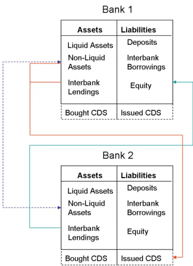
Figure 1 gives an outline of how balance sheets of nancial institutions are interconnected. Solid lines depict direct interconnections while dashed lines depict indirect interconnections. The direction of the arrows indicates exposure towards another bank. For example, the arrow from the interbank lendings of bank 2 to the interbank borrowings of bank 1 represents counter-party exposure of bank 2 towards bank 1.
On the stylized balance sheet from Figure 1 banks' assets consist of liq-uid and non-liqliq-uid assets as well as interbank lendings. Liqliq-uid assets are, for example, cash and cash equivalents. Non-liquid assets are, for example, Collateralized Debt Obligations (CDO) and need to be marked to market if they are held in a bank's trading book. Interbank lendings are, for example, credits given to other nancial institutions. Distinguishing between liquid and illiquid assets is important because one of the main drivers of systemic risk during the recent nancial crisis consisted of banks which were cut o from liquidity on the interbank markets and thus had to sell illiquid assets, resulting in self-energizing resales. Banks' liabilities consist of deposits, in-terbank borrowings, and equity. Below the stylized balance sheets on Figure 1 in dashed lines are conditional assets and liabilities, for example CDS.
To mitigate the risk of future nancial meltdowns it has become con-sensus that, in addition to microprudential supervision, supervisors need
8See Gorton and Metrick (2009) and Gorton (2009) for a detailed analysis of how
Figure 1: Interconnections Between Financial Institutions
to set up an additional layer of macroprudential regulation and supervi-sion which shall allow to identify system-wide risk drivers, monitor systemic risk, and react adequately to it. Systemic risk is a negative externality of nancial institutions on the nancial system. Without charging them for this negative externality, nancial institutions are perversely incentivized to increase their contribution to systemic risk via becoming too-big-to-fail or too-interconnected-to-fail because it allows them to take advantage from re-sulting cheap renancing opportunities.
To analyze systemic risk and banks' contributions to it, we develop a network of interrelated bank balance sheets with endogeneous asset markets. Our model reproduces the main stylized facts with regards to systemic risk that emerged during the recent nancial crisis. We then introduce the con-cept of SVaR in which a Pigouvian tax is used to capitalize a systemic risk
fund. The capital from the systemic risk fund is re-injected into the nan-cial system to make it more resilient to systemic risk. The optimal amount of capital for the systemic risk fund as well as the necessary proportions of capital injected into nancial institutions are determined with a parallelized simulated annealing approach.
Our analysis provides evidence that there is not neccessarily a correspon-dence between a bank's contribution to systemic risk which determines its risk charge and the capital that is injected into it to make the nancial system more resilient to systemic risk. In addition, the analysis provides evidence that a systemic risk fund which is immediately re-injected into the nancial system requires less capital than a systemic risk fund which stores the capital in a central depository and is used to bail out banks ex-post.
The remainder of the paper is organized as follows: Section 2 gives an overview on the previous literature. Section 3 outlines our model, and Sec-tion 4 shows how it can be used to analyze systemic risk as well as individual institutions' contribution to systemic risk along various parameters. Using the outlined model, Section 5 develops and analyzes a proposed systemic risk charge and fund subject to our SVaR concept within a systemic risk man-agement approach. Section 6 concludes. Further details regarding dierent model structures analyzed as well as the parallelized simulated annealing al-gorithm employed for analysis are described in several appendices at the end of the paper.
2 Review of Previous Literature
To get a general overview on systemic risk, Haldane (2009) considers the -nancial network as a complex and adaptive system and applies several lessons from other disciplines such as ecology, epidemiology, biology, and engineering to gain insights to systemic risk in the nancial system. More specically and regarding the various approaches to assessing systemic risk it is sensible to distinguish between (i) `market-based' and (ii) `network-based' approaches.9
While the former use correlations and default probabilities that can be ex-tracted from market prices of nancial instruments, the latter explicitely model linkages between nancial institutions, mostly using balance sheet in-formation.
As regards the market-based literature, Lehar (2005) uses standard tools which regulators require banks to use for their internal risk management however at the level of the entire bank system and shows that in a sample of international banks over the period from 1988 to 2002 the North American banking system increased its stability while the Japanese banking sector has become more fragile. Bartram, Brown, and Hund (2007) develop three distinct methods to quantify the risk of systemic failures in the global banking system. Using a sample of 334 international banks during 6 nan-cial crises the authors come to the conclusion that the existing institutional framework could be regarded as adequate to handle major macroeconomic events. Bårdsen, Lindquist, and Tsomocos (2006) evaluate the usefulness of macroeconomic models for policy analysis from a nancial stability per-spective. They nd that a suite of models is needed to evaluate risk factors because nancial stability depends on a wide range of factors.
To measure systemic risk, more recent research from the market-based literature focuses mainly on detecting systemic risk in groups of nancial institutions, in particular using multivariate measures such as tail risk indi-cators or multivariate distress dependences.10 For example, Gray and Jobst
(2010) nd that using equity option information to calculate (joint) tail risk indicators between institutions yields timely information about the extent of systemic risk. Segoviano and Goodhart (2009) compute the multivariate density of a portfolio of banks to capture linear and non-linear distress de-pendences and apply their methodology to a number of country and regional examples. Among other ndings they show that U.S. banks are highly in-terconnected, and that distress dependence rises in times of crises. Finally, Adrian and Brunnermeier (2009) propose CoVaR, dened as the value at risk
9See the background paper of Financial Stability Board, International Monetary Fund,
and Bank for International Settlements (2009) for a similar distinction.
of nancial institutions conditional on other institutions being in distress to assess systemic risk in the nancial system. Using this measure, the authors quantify the extent to which nancial key gures such as the leverage ratio and maturity mismatch can predict systemic risk.
As regards the network-based literature, Upper and Worms (2004) use balance sheet information to analyze whether there is the risk of contagion in the German interbank market and nd that the failure of a single bank can lead to a loss of up to 15% of the banking system's assets. Cifuentes, Fer-rucci, and Shin (2005) integrate a mechanism of marking to market assets in a network model and show that liquidity requirements can serve as an eec-tive means to forestall contagious defaults in the nancial system. Elsinger, Lehar, and Summer (2006) use standard tools from risk management in com-bination with a network model of interbank loans. Applying their methodol-ogy to a dataset of all Austrian banks they provide evidence that correlations in banks' asset portfolios are a main source of systemic risk. Mueller (2006) employs a data set of bilateral bank exposures and credit lines in a network model and nds a substantial potential for contagion in the Swiss interbank market. Aikman, Alessandri, Eklund, Gai, Kapadia, Martin, Mora, Sterne, and Willison (2009) combine a network model of the nancial system with funding liquidity risk and incorporate this to a suite of models that allow to model various aspects of systemic risk. The authors provide evidence that large losses at some banks can be exacerbated by liquidity feedbacks and thus can lead to system-wide instability.
Castaglionesi and Navarro (2007) study the endogeneous formation of nancial networks and show that an ecient nancial network and a decen-tralized nancial network both display a core-periphery structure in which core banks are all connected among themselves and choose to hold a safe asset while periphery banks can eventually be connected to other banks and choose to hold a risky asset. Gai and Kapadia (2010) develop a network framework where asset prices are allowed to interact with balance sheets. The authors nd that greater connectivity in nancial systems reduces the likelihood of widespread default in case of relatively small shocks, while the impact on the nancial system in case of large shocks increases this likelihood. Espinosa-Vega and Solé (2010) show how a cross-border network analysis can be used to eciently monitor direct and indirect systemic linkages between countries, in particular in the face of dierent credit and funding shocks. The authors provide evidence that the inclusion of risk transfers can modify the risk prole of entire nancial systems.
The recent nancial crisis has revealed that individual nancial institu-tions impact dierently on systemic risk. There are particularly two reasons why it is important to assess nancial institutions' individual contribution to
systemic risk. First of all, to prevent the insecurity surrounding potential de-faults such as the Lehmann bankruptcy in 2008, a supervisor should be able to assess the impact of individual institutions' defaults on the stability of the nancial system. Second, as already outlined in the previous section, individ-ual nancial institutions should be charged to incentivize them to internalize the cost of their negative externality on the nancial system. Tarashev, Bo-rio, and Tsatsaronis (2009) use the Shapley value methodology to identify the contribution of individual nancial institutions to systemic risk. The authors show that none of the drivers of contribution to systemic risk, such as the institution's size or its probability of default, in isolation provide a fully satisfactory proxy for systemic importance. Following the authors, it is thus important to carefully take into consideration the interactions between the various risk factors when analyzing systemic risk and the individual in-stitutions' contribution to it. Gauthier, Lehar, and Souissi (2010) compare alternative mechanisms for allocating the overall risk of a banking system to its member banks. Using a data set of the Canadian banking system the au-thors nd that capital allocations that are optimal with respect to systemic risk can dier by up to 50% from actually observed capital levels. Similarly to Tarashev, Borio, and Tsatsaronis (2009) these allocations are not trivially related to dierent risk factors.
The following section outlines the network model that will be used for our analysis.
3 Model of an Interrelated Financial Network
The model which is set up in this section captures important features of the nancial system and replicates several stylized facts encountered during the recent nancial crisis. It consists of (i) a system of three interconnected nancial institutions that adjust their portfolio to fulll a capital requirement and (ii) the Rest of the World (ROW). Banks have deposits, lend to each other, and hold liquid assets (LA) and non-liquid assets (NLA) on their balance sheet. Non-liquid assets are marked to market11 while liquid assetsdo not change their value on banks' balance sheets. The nancial system is mapped into a matrix of assets and liabilities as displayed on Figure 2.
Figure 2: Matrix of the Financial System Model
Figure 2 summarizes bank balance sheets and their interconnections in a matrix from. The second row, for example, displays bank 1's assets, while its liabilities are captured in the second column. Item 'W' in matrix entry 3/3 represents bank 2's interbank lending to bank 1. W is an asset for bank 2, and a liability for bank 1. Item 'X' represents bank 1's holdings of non-liquid claims on the set of the world like, for example, collateralized debt obligations or corporate loans. Similarly, item 'Y' in matrix entry 2/6 refers to bank1's holdings of liquid assets, i.e. cash and trading book assets. Item 'Z', nally, entails bank 1's deposits and outstanding bonds, held by the rest of the world.
11Note that there is no distinction between banking and trading book in the model, all
Banks have to fulll a minimum capital requirement, γ, which is dened
for bank i according to equation 1,
γ = P jaj +p·bi+ci− P jlj−di P jaj+p·bi , (1)
where i, j ∈ (1,2,3), i 6= j, are indices for the three banks in the system, bi
are non-liquid assets, ci are liquid assets, aj are interbank lendings, lj are
interbank borrowings, p is the market price of the non-liquid asset, and di
are deposits. Note that the liquid asset does not show up in the denominator of Equation 1 because banks do not have to hold capital for their liquid asset holdings.12 If a bank's equity ratio is lower than the capital requirement,
γ, it tries to net its interbank exposure and, if that is not sucient to
ade-quately recapitalize, sells non-liquid assets on the market. In both cases the denominator in Equation 1 decreases relative to the numerator. If a bank cannot meet the capital requirement, it defaults.
Equation 2 shows the capital ratio after netting its exposures against other banks by θ units.
γ∗ = ( P jaj −θ) +p·bi+ci−( P jlj−θ)−di (P jaj −θ) +p·bi (2) Netting reduces the denominator byθ units while the numerator remains
unchanged. Note that in the model, banks may net any cross-exposure as long as their balance sheet equity value remains non-negative, that isP
jaj+
p·bi+ci− P
jlj−di ≥0.13 The term cross-exposure means that two banks
have borrowed from and lent to each other. Note that a bank which has cross-exposure with another bank can have net-cross-exposure with the same bank. Here and in the following net-exposure is dened as one bank having lent more to another bank than borrowed from the same bank.
Solving Equation 2 for the amount of banki's desired netting yields
Equa-tion 3 θdi =−111[nvi≥0] (1−γ)(P jaj +p·bi+ci− P jlj−di) γ , (3)
where 111 is an indicator function and nvi is bank i's net-value dened as P
jaj+p·bi+ci− P
jlj−di. The amount of netting the j'th bank is willing
to accept with bank i is given by Equation 4
θsj = 111[nvj≥0]min(ai, li). (4)
12See Cifuentes, Ferrucci, and Shin (2005) for a similar set up.
13If a bank's liabilities exceed its assets, it is taken into custody by the supervisor to
Note that the minimum operator is used since only cross-exposures can be netted. The resulting amount netted between bank iand bank j is given by
Equation 5
θji =min(θjs, θ d
i). (5)
Note that in the model banks never increase their lending to each other. Furthermore, in order to meet the minimum capital requirement, the bank may engage in asset sales. Equation 6 shows the capital ratio bankiexpects
to obtain if it engages in selling si units of its non-liquid assets.
γ∗ = P jaj +p(bi−si) +ci+p·si − P jlj −di P jaj+p(bi−si) (6) Consider the indirect eects of the above responses to violations of Equa-tion 1. Netting by bank i increases γ for banks i and j, where bank j is
holding the cross exposure. Asset sales by bank i, in contrast, have further
repercussions on all banks with positive exposure14 in that very asset,
be-cause asset sales have an impact on its secondary market price. In the model it is assumed that market prices of non-liquid assets, p, are a function of
supply and demand on the market. If banks engage in liquidating (part of) their non-liquid assets, several eects on banks' balance sheets have to be considered: the seller obtains cash, a liquid asset, and hence improves her capital ratio. However, at the same time an increased supply of non-liquid assets to the market decreases the market price of the asset, lowering the market value of the bank's remaining portfolio holdings of the same asset. Furthermore, the price eect also inuences other banks' balance sheets since the market value of their non-liquid assets is reduced as well.
In the model, the market price of the non-liquid asset is found via a tâton-nement process between supply and demand. Following Cifuentes, Ferrucci, and Shin (2005), the inverse demand function is assumed to follow Equation 7
p=exp(−ξX
i
si), (7)
where ξ is a positive constant to scale the price responsiveness with
re-spect to non-liquid assets sold, and si is the amount of bank i's non-liquid
assets sold in the market.
Solving Equation 6 for the amount of non-liquid assets sold by bank i to
fulll the capital requirement, and noting that a bank can only sell non-liquid
14We restrictbito be non-negative, assuming that bank asset holdings refer to cash ow
streams outside the nancial sector. Put dierently, bonds issued by banks are included in lj.
assets it holds in positive quantities15, leads to Equation 8. It shows banki's
supply of non-liquid assets on the market as a function of the market price.
si =min bi, −(1−γ)(p·bi+ P ai)−ci+ P li+di γp (8) Since each si is decreasing in p, the aggregate sales function, S(p), is also
decreasing in p. The tâtonnement-process leading to the equilibrium market
price is depicted in Figure 3.
Figure 3: Tâtonnement Process in the Model
Prior to any shock, the market price equals 1, which is the initial price when all banks fulll their respective capital requirements, and sales of the non-liquid asset are zero. A shock to bank i, say a certain loss of cash, ci, shifts the supply curve upwards, resulting in S(1) = si 0 because
15Note that banks do not engage in buying or short-selling non-liquid assets in the
bank i starts selling non-liquid assets to fulll its capital ratio. However, for S(1) the bid price equals only p(S(1))bid, while the oer price is one.
The resulting market price is p(S(1))mid, the midprice between bid and oer
prices. Since the market price thus decreases and banks have to mark their non-liquid assets to market, additional non-liquid asset sales may be needed to fulll the capital requirement. The stepwise adjustment process continues the demand and the supply curves intersect atp∗. Note that the supply curve
may become horizontal from some value of non-liquid assets sold onwards, as the total amount of non-liquid assets on the banks' balance sheets is limited. Since a shock to a bank will always result in an upward shift of the supply curve, and the maximum price of the non-liquid asset being equal to 1, while the initial equilibrium prior to the shock equals zero, a market pricep∈(0,1)
always exists.
In the framework just outlined, there are two main shock transmission channels, the direct connection between banks via interbank holdings (credit risk), and indirect connections via marking to market of non-liquid assets on the balance sheet (market risk).
The following sub-section explains how dierent congurations of a nan-cial network can be captured in the model.
3.1 Generating Specic Realizations of the Financial
System Matrix
Any specic set up of a nancial system is described by a consistent matrix, that is, when all banks fulll their capital requirement ratio, with concrete values for all assets and liabilities, as depicted in gure 2. Accordingly, a setup is dened by (i) the structure of the system, that is, the network of exposures and cross-exposures among banks and the rest of the world; (ii) the banks' individual ratio of interbank lending to other assets (that is, her non-liquid and liquid asset holdings), α, with α the overall amount lent to
other banks, and 1−αthe amount invested in other assets; (iii) the ratio of
investment in non-liquid to liquid assets, β, whereβ is the fraction invested
in non-liquid assets and 1−β is the fraction invested in liquid assets; (iv)
the capital requirement, γ; and (v) an initial endowment of capital, A, that
is allocated to banks' assets according to α and β. Note that 0≤α ≤1 and 0≤β ≤1.
To determine all except the last row of the nancial system matrix in Figure 2, the structure of interlinkages, i.e. the net of exposures has to be dened, and concrete values for α, β, A, and γ have to be assigned. In the
and non-liquid assets. The overall amounts bank i holds in non-liquid and
liquid assets are ((1 −α)· A+P
jlj)β and ((1 −α)· A+ P
jlj)(1 − β),
respectively. The entry for the i'th bank in the last row of the nancial
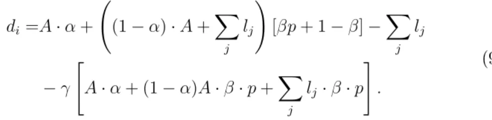
system matrix, that is, its deposits, is residual in the sense that the capital requirement is just met, using Equation 9
di =A·α+ (1−α)·A+ X j lj ! [βp+ 1−β]−X j lj −γ " A·α+ (1−α)A·β·p+X j lj ·β·p # . (9)
As an example, Figure 4 illustrates the symmetric case. All banks have identical initial capital, A, they borrow from and lend to each other, and they have identical portfolio allocations, α and β.
Figure 4: Symmetric Case of the Financial System Matrix
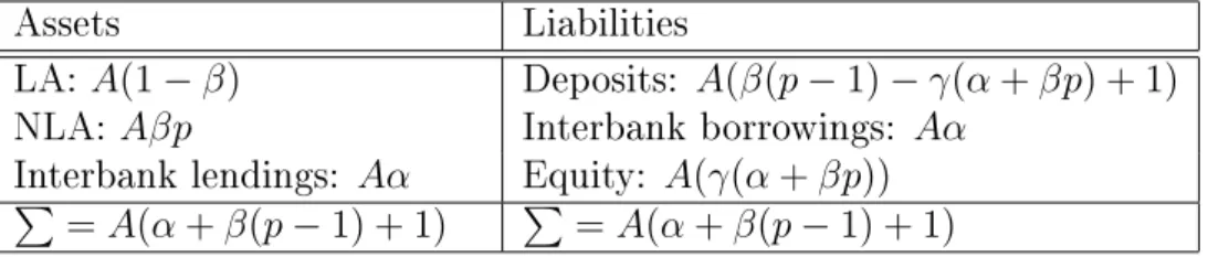
In the example on Figure 4 each bank's balance sheet then looks as dis-played on Table 1.
Note that with dierent interlinkage structures the relative size of banks vis-à-vis each other, measured by the sum of their assets, changes because banks choose their leverage independently, and are free to select their desired balance sheets.
The next sub-section outlines how shocks to the nancial system matrix are modeled.
Assets Liabilities
LA: A(1−β) Deposits: A(β(p−1)−γ(α+βp) + 1)
NLA: Aβp Interbank borrowings: Aα
Interbank lendings: Aα Equity: A(γ(α+βp)) P
=A(α+β(p−1) + 1) P
=A(α+β(p−1) + 1)
Table 1: Banks' Balance Sheets in the Symmetric Case
3.2 Shocks in the Financial System Matrix and the
Mea-sure for Systemic Risk
As explained in the beginning, systemic risk is dened as the hazard of bank failures causing a decrease in the supply of credit and nancial services to the economy which, resulting in negative real eects. Accordingly, we dene systemic risk conditional on a shock as the relative size of the nancial system that breaks down. It is measured by the banks' balance sheet size, that is, the sum of their assets. Intuitively, when banks default, the resulting liquidation costs as well as the the banks' overall importance to the real economy will be closely related to the size of its balance sheet.
Shocks in the model come in the form of percentage loss in asset val-ues. The resulting systemic risk is calculated as the ratio of assets from defaulting banks to system-wide asset total, both measured prior to the shock. For example, if subsequent to a shock only bank 1 defaults, while all other banks in the nancial system remain solvent, then systemic risk is
Sum of Bank 1's Assets Prior to the Shock Sum of all Banks' Assets Prior to the Shock.
A wide range of possible shock events, from mild to severe, are considered in the simulations. Strongly adverse scenarios with high unexpected losses will be included among these scenarios, as such shocks are likely candidates to trigger systemic risk events, involving defaults of parts of the nancial system. The expected systemic risk in a particular point in time is calculated as the weighted sum of systemic risk events caused by a distribution of shock realizations. The weights are derived from the probability distribution of shock realizations. Equation (10) denes this measure of expected systemic risk.
ΦE =X
j
Sum of Insolvent Bank's Assets Prior to Shockj
Sum of all Banks' Assets Prior to Shockj
·probj (10)
where ΦE is expected systemic risk and prob
j is the probability assigned to
shock scenarioj. Dening systemic risk this way, i.e. assuming a distribution
individual banks to overall systemic risk. At the same time, it allows to handle the three main risk-channels of interbank risk in a unied framework, namely bank size, bank interconnectedness, and bank asset re sales. As it turns out, given the parametrization chosen in our model, the re sale channel is particularly sensitive to systemic risk, since even small shocks have a signicant eect on nancial system default rates. The interlinkage channel, on the other hand, requires a relatively large shock to generate a system-wide default. Our modeling strategy allows to adopt the Value at Risk (VaR) metros,16 the standard risk management tool used in microprudential
supervision, for a macroprudential problem. The resulting metric, the System Value-at-Risk (SVaR), is eectively a set of stress tests for an entire banking system. This metric, expected systemic risk, will be used subsequently to analyze systemic risk in the nancial system.
Each possible shock to the banking system is modeled as a vector of per-centage losses to a bank's (non-weighted) sum of assets over a discrete grid,
ι, ranging from 1% toς%, withς being the highest conceivable shock.
Con-sidering all combinations of shocks for the three banks yields a total number of ι3 shock vectors. Each shock vector consists of n elements, i.e. the loss
associated with the shock for each institution our model with n banks. In
this paper,n=3. The probability of a shock realization is captured by a
multi-variate normal distribution centered at a value between 1 and ς. The extent
of correlation between the shocks is modeled with the variance-covariance matrix of the multivariate normal density function. The correlation between shocks in a given scenario, say a shock to banks 1 and 2 in scenario 1, is then calculated as cov1,2
σ1σ2 , where cov1,2 designates the covariance between shocks 1
and 2 and σ1 and σ2 are the standard deviations of shocks to banks 1 and
2, respectively.17 Since shocks only range from 1 to ς, the multivariate
nor-mal density is rescaled such that the integral of the volume described by the discrete grid of shocks, ranging from 1 to ς in all three dimensions equals 1.
As previously outlined, if subsequent to a shock realization, the bank cannot fulll its capital requirement, it will net its counterparty exposures rst. Next, if netting is not enough to meet the capital constraint, the bank will sell non-liquid assets, thereby indirectly transmitting the shock to other banks, via a downward pressure on the market prices of non-liquid assets. If it still cannot fulll the capital requirement,the bank will go into defaults. In default, seniority of deposits over other liabilities is respected.
The clearing algorithm for shock transmission is an iterative process in
16See Jorion (2006) for an outline of the VaR methodology.
17Apart from the resale channel for non-liquid assets, the correlation between direct
shocks to dierent banks captures an additional element of common bank exposure within the nancial system.
which banks sequentially absorb the shock. Banks initially try to fulll their capital requirement via netting counterparty exposures, and, after that stage, via selling non-liquid assets into the market. Banks with negative net-value, i.e. negative equity then transmit a shock to their creditors, and the iterative process restarts. The process ends when shocks to solvent banks are fully absorbed. Figure 5 depicts the procedure of modeling the shock transmission.
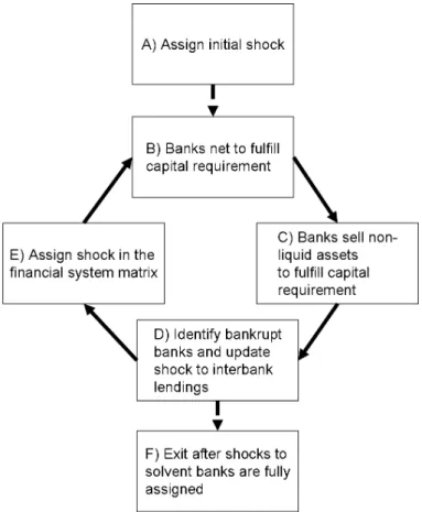
Figure 5: Shock Transmission in the Financial System Model
Banks' assets are contracted by the initial shock (step A on Figure 5). Banks that do not fulll the capital requirement rst try to improve their capital ratio through netting interbank liabilities with other banks, since netting has no negative repercussions on the balance sheet (step B on Figure 5). Next, banks that still do not fulll the capital requirement start selling non-liquid assets in the market (step C on Figure 5).
Banks that are not able to fulll the capital requirement even after selling all their non-liquid assets, will enter into default. If insolvent banks have negative net-value they will transmit shocks to their creditors, that is, banks
that have exposure with them, or ultimately to the bank's depositors. A bank with negative net-value transmits shocks to its creditors, respecting seniority, until it has a net-value of zero. The overall shock prepared for transmission to the insolvent banks' creditors equals the absolute value of their negative net-value and is assigned proportionally to a bankrupt's bank interbank liabilities as long as they are positive (step D on Figure 5).
In case the interbank liability shock matrix contains nonzero entries it is assigned (step E on Figure 5), and the iteration restarts (step A on Figure 5). If the interbank liability shock matrix is empty the shock has been assigned, and the resulting systemic risk is computed (step F on Figure 5).
The following sub-section outlines how the model can be used to analyze individual nancial institutions' contribution to expected systemic risk.
3.3 Analyzing Banks' Contribution to Expected
Sys-temic Risk
To identify the contribution of an individual bank to expected systemic risk, the Shapley value methodology can be employed.18 In game theory this
value is used to nd the fair allocation of gains obtained by cooperation among players. For a game consisting of three players the Shapley value is dened as φi(v) = X K3i;K⊂N (k−1)!(n−k)! n! [v(K)−v(K− {i})], (11)
where k is the number of players in coalition K, N is the set of all players,
v(K) is the value obtained by coalition K including player i and v(K− {i})
is the value of coalition K without player i. The Shapley value for player i
is the average contribution to the gain of the coalition over all permutations in which players can form a coalition.
The analogy between gains allocation in game theory and systemic risk contribution in nancial economics is evident, as individual banks through their portolio structures and their interconnections to other banks and to the rest of the world may increase or decrease the likelihood of a given nancial
18See Shapley (1953). Tarashev, Borio, and Tsatsaronis (2009) also rely on the Shapley
value to compute individual nancial institutions' contribution to systemic risk. Note that in general also other measures for nancial institutions' contribution to systemic risk could be employed, for example the CoVaR methodology developed by Adrian and Brunnermeier (2009). However, for a simulation based approach to systemic bank risk, the Shapley value methodology is suited particularly well, as dierent patterns of interbank dependencies, i.e. via portfolio structures and via interbank lending and borrowing, can be accounted for. The CoVaR methodology, in comparison, relies on reduced form representation instead.
system experience multiple bank defaults. In this sense, a bank's contribution to overall system risk can a priori be positive or negative. Furthermore, the marginal eect of a bank on overall systemic risk cannot be estimated from bank-individual data alone; the interplay with other banks' balance sheets and their portfolio compositions is needed to assess the bank's impact on system stability.
The Shapley value has a number of well-known properties:
• Pareto eciency: The total gain of a coalition is distributed;
• Symmetry: Players with equivalent marginal contributions obtain the
same Shapley value;
• Additivity: If one coalition can be split into two sub-coalitions then
the pay-o of each player in the composite game is equal to the sum of the sub-coalition games;
• Zero player: A player that has no marginal contribution to any coalition
has a Shapley value of zero.
Of course, expected systemic risk is a cost to the nancial network. There-fore, the Shapley value can be employed to to compute the marginal contri-bution of any single bank to the overall cost of systemic risk.
From the nancial network matrix, the contribution of each single bank to systemic risk is determined in Equation 11, given a shock of a particular magnitude. As outlined before, systemic risk conditional on the realization of a shock is dened as the proportion of the assets of all banks that enter default because of a system wide asset shock, where pre-shock asset values are used to dene the proportions. v(K) is the coalition K of `all banks
that can default and transmit shocks' and hence contribute to the measure for expected systemic risk, and v(K − {i}) is the coalition K without the i'th bank. Intuitively, the latter can be imagined as the situation in which
bank i cannot default and thus not transmit shocks to the nancial system.
In the model this is done via temporarily adding a large amount of liquid assets to a bank that shall not transmit shocks. Such a 'safe' bank does not try to net counterparty exposure19 or sell non-liquid assets on the markets
because it always fullls the capital requirement. Following this approach, one calculates for each permutation of banks the systemic risk if only the rst bank in the order can default, next the marginal contribution to systemic risk if the following bank can also default, and nally the marginal contribution to
systemic risk if all three banks in the actual order can default. The Shapley value for a bank is then the average of its marginal contributions over all possible permutations. Since systemic risk is dened as a proportion here, its value and the Shapley values are restricted to lie between 0and 1.
Similar to calculating expected systemic risk as a weighted sum of sys-temic risk from a set of scenarios, Equation (12) outlines banki's contribution
to expected systemic risk from a weighted sum of its Shapley values.
φEi =X j
φij ·probj (12)
where φij is bank i's contribution to systemic risk in scenario j and probj is
the probability that scenario j realizes. Note that ΦE =P3 i φ
E i .
Using the model just developed, the nest section analyzes the main de-terminants of systemic risk.
4 Applying the model: Systemic risk and its
determinants
In the model banks' contribution to expected systemic risk is driven in partic-ular by three characteristics, namely a bank's size within the nancial system, as well as the extent of direct and indirect links among the banks.20 First
of all, the size of an individual bank matters for its contribution to expected systemic risk because our measure of systemic risk, total assets of defaulting banks relative to system-wide assets, both measured prior to the shock real-ization, increases with the size of the 'shocked' bank's balance sheets. Second, banks that have borrowed from other banks are likely to contribute more to expected systemic risk than banks inactive in interbank borrowing. Further-more, a defaulting bank with outstanding interbank liabilities transmits a shock to its creditor banks. Third, with signicant amounts of non-liquid assets on banks' balance sheets, the nancial system becomes vulnerable to re sales. Non-liquid assets on a bank's balance sheet creates vulnerabilities with respect to movements of asset prices. Furthermore, subsequent to a loss, banks may be forced to sell non-liquid assets, thereby furthering the downward spiral of asset prices and transmitting the shock to other banks in the nancial system. The following analyses will consider these three main risk-channels in turn.
Expected systemic risk will rst be explored in a baseline specication of the model. Subsequent analyses will then investigate the impact of the above risk-channels. To shed some light on the role of banks' capitalization and its role as a shock buer, the eect of dierent capital requirement ratios on expected systemic risk will also be investigated.
In the baseline specication parameters are set such that banks' resulting balance sheets roughly corresponds to the proportions actually found in a real-word nancial system. Concerning the relative importance of interbank lending, Upper and Worms (2004) in their study on the German interbank market report an average level of interbank lending of 2.96 times the amount of their own capital. Scaling the parameter α to 0.3 in our model generates
approximately the aforementioned relative amount of interbank lending, as-suming the bank engages in such lending at all. Furthermore, the proportion of non-liquid assets to cash and cash equivalents at an international univer-sal bank, as for example Deutsche Bank in 2009 was roughly 0.8.21 In the
model, we setβto0.8, roughly mimicking the proportion found at an
interna-20Throughout the remainder of the paper we will refer to expected systemic risk caused
by direct and indirect interconnections as `interlinkage' and `resale' channels, respectively.
tional bank. As regards banks' capitalization, following the Basel Commitee on Banking Supervision (2006), the capital requirement ratio, parameter γ,
is set to 8% of risk weighted assets, where we assume risk weights to be uniformly one for non-liquid assets, and zero for liquid assets. The scaling parameter for the price responsiveness of non-liquid assets, parameter ξ, is
set to 0.03which results in a price decrease of approximately 7% of its
mar-ket price if banks sell all their non-liquid assets on the marmar-ket. Banks in the system are initially equipped with one unit of capital, parameter A. Since
systemic risk is measured as a proportion throughout the following exercises,
A is eectively a scaling parameter. It aects results only if banks were to
obtain dierent amounts of initial capital because only then banks' relative sizes will be aected.
To repeat, shocks that aect individual banks are modeled as a loss of a bank's assets ranging from 1% to 9% of its balance sheet sum in discrete steps of 2%. Note that a shock always manifests itself via a loss in liquid asset value.22 The multivariate normal shock distribution which determines
the shock scenario realizations is centered at a loss of 6% of banks' assets.
The main diagonal of the variance-covariance matrix is set to 3, and the
covariances are set to yield a pairwise correlation coecient of 1
6 between
shocks to all banks.23
Note that the distribution of shock scenarios will likely inuence the out-comes of the following analyses. For example, choosing the parameters of the distribution such that small shocks receive a relatively high likelihood will generally reduce the expected risk contribution of the interlinkage channel. This property of the mechanism is due to the fact that banks only transmit shocks via the interlinkage channel if a shock is large enough to reduce the sum of a bank's assets below the sum of its liabilities, that is, its equity is exhausted. Similarly, if very large shocks have a high probability, the size channel dominates the outcome as regards banks' contribution to expected systemic risk. In the extreme case when all banks lose all equity from an initial shock and cannot recapitalize, the whole banking system defaults. In
22A direct loss assigned to non-liquid assets might aect the resales channel in the
model. A larger shock to an institution's non-liquid assets can theoretically cause lower risk in the nancial system through a reduced volume of resales. In the extreme case of a bank losing all its non-liquid assets subsequent to a shock, its potential to transmit the shock via the resales channel has vanished.
23Concerning mean and variance of the shock distribution, there is little empirical
guidance as to how these parameters can be chosen. Moody's Investor Service (2005) estimates the asset correlations for major structural nance sectors to range between 2% and 18%. Given that the recent nancial crisis has demonstrated that correlations in the nancial sector can be even higher than was previously assumed, a value slightly above the upper range of the interval has been chosen.
this case, there is no room for contagion via resales, or interlinkages. In this respect, the variance and covariance of shocks matter as well. For example, to identify banks which contribute to expected systemic risk via the interlink-age channel it is necessary to model shock scenarios in which creditor banks are subject to a relatively small shock. 'Small' implies it does not cause the bank to default, even if, at the same time, its debtor banks are subject to a relatively large shock which makes them default on their liabilities. thus ultimately imposing some default risk on creditor banks. The distribution parameters thus inuence expected systemic risk directly as well as indirectly, through banks' systemic risk contributions, via dierent channels.
Our choice of parameters governing the distribution of shock scenarios has been taken mainly with a view on generating shock scenarios which, on the one hand, allow for the emergence of systemic risk through all risk-channels, and, on the other hand, to identify through which of the channels banks primarily contribute to expected systemic risk. It is important to note that while the analyses are in some cases aected by distributional assumptions and interactions between the risk-channels themselves, the insights obtained from the outcomes of the experiments are qualitatively robust to changes in these underlying parameters because they are always corroborated with a view on the model's underlying mechanics. Furthermore, in case the distri-butional assumptions particularly matter, we will discuss the robustness of the results in question.
Given that a bank can engage in borrowing and lending to and from other banks simultaneously, there exist26possible banking structures, i.e. patterns
of interbank exposures. Appendix A, at the end of the paper,describes all possible structures of the nancial network matrix.
In the next section, the properties of a model of interconnected banking with endogenous asset markets is explored using a baseline specication. The role of dierent channels of risk contagion in the emergence of systemic risk is analyzed. The discussion will be in terms of bank 1's contribution to systemic risk. This is without loss of generality since the interlinkage structures as seen from banks 2 and 3 are symmetric, and it therefore suces to report results from the view of one bank only. For example, as can be seen in Appendix A, structure 19 from the perspective of bank 1 is the same as structure 25 from the perspective of bank 3.
Finally note that all following analyses will frequently refer to specic structures of the nancial system as well as to banks' size, counterparty exposure, and amount of non-liquid asset investment. Besides the general structural overview given in Appendix A, a presentation of specic banking network structures as well as their size distribution can be found in Appendix B, along with banks' relative size.
The following sub-section analyzes expected systemic risk in the baseline specication.
4.1 Expected Systemic Risk in the Baseline
Specica-tion
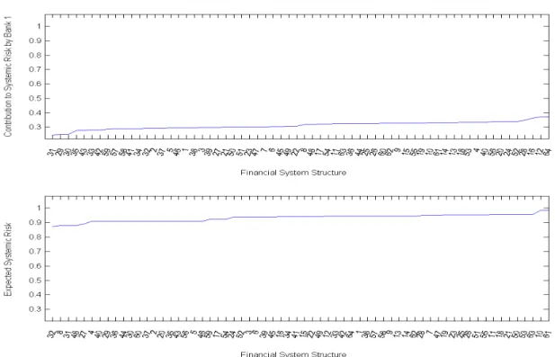
Figure 6 displays expected systemic risk in the baseline specication of the model. The upper panel shows the contribution of bank 1 to expected sys-temic risk (y-axis). The possible interlinkage structures outlined in Appendix A have been ordered from lowest to highest contribution to expected systemic risk (x-axis).
In the baseline model, it is interlinkage structure 31 in which bank 1 contributes least to expected systemic risk (Table 13 in Appendix B). Looking at the three main risk-channels, i.e. size, interlinkages, and resales, suggests why this is the case. First of all, in this network structure, bank 1 is relatively small, holding merely 28% of total assets in the nancial system. Second, it has no direct connections to other banks. This prevents it from being involved in shock transmissions via interbank lending. Third, in this network structure, bank 1 holds the same amount of non-liquid assets as the other two banks and thus is not particularly involved in the resales channel either. At the other end of the spectrum are network structure 12 and 64, in which Bank 1 is the major contributor to expected systemic risk (Tables 7 and 16, respectively). Here, bank 1 holds 36% of nancial system total assets. It thus contributes more prominently to expected systemic risk via the size channel. Furthermore, due to its interlinkages with other banks in both network structures, it can directly issue or indirectly transmit a shock to its creditor banks. Finally, in this network structure, bank1 has a major amount of non-liquid assets on its balance sheet, rendering participation in resales more likely.
As outlined at the beginning of this section, expected systemic risk and bank 1's contribution to it may depend on the distributional assumptions of the shock scenarios. Note, for example, that in structure 16 (Table 8), though bank 1 is the largest bank in the nancial system (44%), two banks have net-exposure to it, and it has the largest holdings of non-liquid assets, it contributes slightly less to expected systemic risk than in structures 12 or 64. This result is due to the fact that shocks large enough to throw several banks into default, as in network structure 16, are at the extreme end of the shock distribution and thus receive relatively little weight in the calculation of expected systemic risk (Equation (10)).In this particular scenario, Similarly, bank 1's contribution to overall systemic risk is limited (Equation (12)).
In contrast, in network structures 12 or 64, an eventual loss from bank 1 is transferred forcefully to its single creditor, rendering a sigincant shock transfer more likely, particularly for relatively smaller shocks with a higher probability weight in the shock distribution.
The lower panel in Figure 6 displays expected systemic risk (y-axis) in the nancial system over the dierent possible interlinkage structures (x-axis). The structures have been ordered by expected value of systemic risk. In the baseline specication expected systemic risk is lowest in interlinkage structure 32 (Table 14), where banks are not connected at all by interbank lending, and are otherwise equal with respect to size, and non-liquid asset holdings. Expected systemic risk peaks when network structures display unidirectional links, as for example in structures 10 and 61 (Tables 6 and 15, respectively). Note that in these structures, the arrows are `pointing' into the same direction, that is, from bank 1 via bank 2 to bank 3, and from bank 3 back to bank 1, or vice versa, such that each bank can send shocks via interbank linkages to all other banks in the nancial system. In these network structures with maximal risk, banks are akin with respect to size and non-liquid asset holdings.
We now turn to the main risk-channels for the emergence of expected systemic risk. The systemic risk contribution of individual banks will be analyzed in the next sub-section. To isolate the eect of any particular chan-nel, we will modify the simulations such that other channels are temporarily (partially) shut down. Note that the size variations in our model do hinge upon initial amounts of capital, A, as well as upon bank interconnectedness,
since bank borrowings increase the scale of their operations.
The next sub-section analyzes the eect of resales on expected systemic risk.
4.2 The Eect of Firesales on Expected Systemic Risk
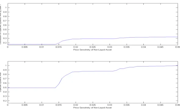
The eect of the `resales' channel on expected systemic risk can be analyzed if the `interlinkage' channel is shut down and all banks start with the same amount of initial assets. This can be done using structure 32 (Table 14), where all banks have the same size with respect to the nancial system and do not lend to each other. The price responsiveness of the non-liquid asset, parameter ξ, is increased from 0 to 0.05. If all non-liquid assets are sold on
the market, the percentage loss of the price of the non-liquid asset then ranges from 0% to 11%, respectively. Figure 7 displays the eect of an increase in the price responsiveness of the non-liquid asset (x-axis) on expected systemic risk (y-axis) on the lower panel and bank 1's contribution to it (y-axis) on the upper panel, both in structure 32. Not surprisingly, the impact of the resale
Figure 6: Expected Systemic Risk in the Financial System Model's Baseline Specication
channel depends upon the price sensitivity of secondary asset markets to an increase of sales. High price sensitivities translate into increased expected systemic, while bank 1's contribution rises as well. For parameter value of 0.05 and above, even small shocks to asset value may translate into the default of the entire nancial system.Because relatively small amounts of non-liquid assets sold in order to recapitalize the balance sheet may lead to signicant price eects, triggering a resale spiral.
Note that the functions displayed on Figure 7 do not follow a smooth pattern because of the coarseness of the grid of shocks, featureing a stepsize of 2% over a range of losses. For example, assume that given price respon-siveness, a bank losing 5% of its assets is not able to recapitalize successfully, and thus is forced to sell all its non-liquid assets on the market before default-ing. If the price responsiveness is then ceteris paribus slightly increased, this bank would start liquidating its assets earlier, say at a loss rate of 4% before defaulting. However, since the next smaller shock considered is 3%, the price responsiveness needs to be raised sizeably to increase expected systemic risk and banks' contribution to it over some ranges of the grid. The upshot is
Figure 7: Eect of Firesales on Expected Systemic Risk in Financial System Structure 32
that over some regions of the parameter space of ξ, a signicant increase in
price elasticity is required to cause an osetting increase in expected systemic risk.
The simulation results presented in this section suggest the importance to understand the price elasticity of non-liquid assets in order to estimate ex-pected systemic risk properly. The same holds true for a bank's contribution to systemic risk.
The next section turns to the role of interbank lending in the emergence of systemic risk.
4.3 The Eect of Interlinkages on Expected Systemic
Risk
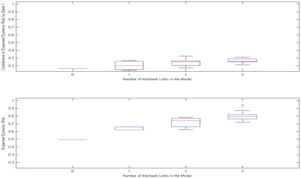
As a rst inspection of the eect of interlinkages on expected systemic risk, Figure 8 displays a boxplot of expected systemic risk (lower panel) as well as bank 1's contribution to it (upper panel), for dierent number of interbank links, according to the 64 possible nancial network structures in the model. Note that two banks are considered as being connected if there is a single link
between them. To focus on the pure eect of interbank connectedness, we have to abstract from other risk determinants, like asset resales and bank size. Therefore, the parameter of price responsiveness has been set to zero, and initial assets of bank j is equal for all banks. Results are presented in a
Figure 8: Eect of Number of Interlinks on Expected Systemic Risk box plot diagram. When investigating the medians (red lines), the plots sug-gest that expected systemic risk, as well as bank 1's contribution to it, tend to increase with the number of active links across banks. However, focusing on the upper and lower quartiles (designated by the blue boxes), the whiskers which extend to the extreme data points (black lines), and to outliers (red plus symbol), demonstrate that there is no monotonous relationship between number of interbank links and expected systemic risk, or contribution to it. In the network literature this property is sometimes labeled 'robust, yet fragile', meaning that a growing number of interbank linages will render the network more robust vis-à-vis small shocks, and at the same time more vulnerable to large shocks. Since in this case the shock vectors are the same, the `robust yet fragile' property follows from a specic network structure, namely cross-exposures between two banks, akin to a mutual insurance.
The box-plots in Figure 8 suggest that expected systemic risk as well as a bank's contribution to it increase with the number and the intensity of
Figure 9: Eect of Financial System Structures on Expected Systemic Risk interlinkages in the nancial system.
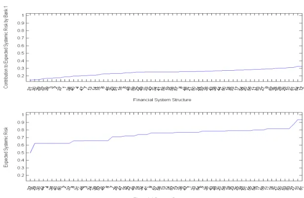
As an alternative representation, the eect of the interlinkage-channel on expected systemic risk is presented in Figure 9 analogously to Figure 6. It again relies on the baseline specication, but this time the resales channel is shut down. In other words, the parameter for price responsiveness, ξ, is set
to zero, while all banks are starting with the same amount of initial assets, parameter A.
Qualitatively the results remain broadly the same. However, two points deserve mentioning. First, in Figure 9 expected systemic risk (lower panel) as well as bank 1's contribution to it (upper panel) turn out to be lower than before. For some structures with a low level of expected systemic risk, such as structure 32, the decrease of expected systemic risk (from 0.87on Figure
6 to0.49on Figure 9) and bank 1's contribution to it (from0.29on Figure 6
to0.17on Figure 9) are signicant. For other structures, such as for example
structure 61 which is at the high end of expected systemic risk, the eect is relatively small (expected systemic risk decreases from 0.99 on Figure 6 to 0.94 on Figure 9 and bank 1's contribution to it from 0.33 on Figure 6 to 0.31on Figure 9.).
Second, the ordering of structures along the x-axis can be aected, provid-ing further evidence that the resales channel impacts expected systemic risk arising through dierent interlinkage structures to dierent extents. Shock transmission via direct interlinkages takes only place if a debtor bank is hit by a shock which is strong enough to turn the bank's net-value negative because the direct interlinkage channel only gets contagious once the debtor bank's equity has been completely extinguished. The analysis of Sub-Section 4.2 has already provided evidence that the resales channel increases the impact of shocks, as, for example, a high value for the parameter for price respon-siveness, ξ, causes the whole nancial system to default at even tiny shocks.
This feature indirectly also impacts the eect of interlinkages and can thus aect expected systemic risk as well as banks' contribution to it in some structures.
Consider, for example, expected systemic risk and bank 1's contribution to it in structures 19 and 25 (Tables 9 and 10, respectively) on Figures 6 and 9. Both structures yield the same expected systemic risk on the same gure (0.96on Figure 6 and0.79on Figure 9.). However, comparing bank 1's
contributions to expected systemic risk (upper panel) on Figure 6 with the resales channel being active, bank 1 contributes less to expected systemic risk in structure 25 (0.32) than in structure 19 (0.33). By contrast, with the resales channel shut down, on Figure 9 bank 1 contributes relatively more to expected systemic risk in structure 25 (0.30) than in structure 19 (0.25).
This change in the relative magnitudes of systemic risk attached to partic-ular network structures are a consequence of the interaction between lending (cross-) exposures and asset resales, as well as the mean shock size. The underlying mechanism can be investigated by quantifying the risk-channels through which bank 1 contributes to expected systemic risk. Considering the interlinkage channel in isolation, bank 1's contributions to expected systemic risk are considerably larger in structure 25 than in structure 19.24
Further-more, in structure 25 bank 1 constitutes a larger proportion of the nancial system (0.37) and has more non-liquid assets (0.92) than in structure 19 (0.33 and 0.8, respectively). Depending on the shock scenario, bank 1 can
24As can be seen on Tables 9 and 10, in structure 25 bank 3 has net-exposure to bank
1 and bank 2 has net exposure to bank 3, while in structure 19 bank 2 has net-exposure to bank 1 and bank 1 has net exposure to bank 3. This means that in structure 19 bank 1 can directly send a shock to bank 2 and/or transmit a shock from bank 3 to bank 2. In structure 25, however, bank 1 can directly send a shock to bank 3 which will transmit the shock even further to bank 2. Ceteris paribus, in the model a bank X that transmits a shock to another bank Y, which inn turn forwards the shock to a third bank Z contributes more to systemic risk than a second bank X which sends a shock to another bank Y but also forwards a shock from one bank Z to another bank Y.
contribute more to systemic risk in structure 25 than in structure 19, across all three channels.
This is reected on Figure 9 where bank 1 contributes more to expected systemic risk in structure 25 than in structure 19. Note that when the resales channel is shut down, the interconnection channel is generally weak in the baseline specication. It therefore merely plays a minor role in this bank's contribution to expected systemic risk.25 We summarize these observations
by stating that bank 1's larger systemic risk contribution in structure 25 as opposed to structure 19 in Figure 9 is apparently driven by the larger size of bank 1 in scenario 25.
Furthermore, according to Figure 6, bank 1 contributes slightly more to expected systemic risk in structure 19 than in structure 25. The change of order between the two structures when the resales channel is active ren-dering shocks more severe can be traced to the properties of the shock distribution.26 Since shocks close to the mean receive a higher probability
weight in the computation of the contribution to expected systemic risk than shocks on the upper range of the interval of shocks analyzed, bank 1 con-tributes more to expected systemic risk via the interlinkage channel which in this case outweighs its relatively smaller contribution from the other two channels in structure 19 than in structure 25 on Figure 6.27
Shutting down the resales channel also has mixed eects on expected systemic risk, depending on the actual network structure of the nancial system (lower panels on Figures 6 and 9). For example, the second lowest expected systemic risk is found in structure 8 (0.88; Table 5) on Figure 6. This structure is relatively safe because only banks 1 and 3 which have
cross-25Banks that have borrowed from other banks to invest into non-liquid assets are
rela-tively safe, given the resales channel shut down, because non-liquid assets are similar to liquid assets in these circumstances.
26With the resales channel open, shocks to banks in the nancial system have more
impact, increasing also the inuence of the interconnection channel. Taking into account the mean size of shocks to the system, a further needs to be considered: a large shock to bank 1, that is, a shock on the upper range of the shocks considered, to bank 1, quickly erases equity such that the bank cannot use netting anymore to reduce its counterparty exposures. In case of a medium shock to bank 1, i.e. a shock close to the mean of the shock distribution, equity will not be wiped out, so it may improve its capital ratio via netting. Since bank 1 can net more counterparty exposure in structure 25 (0.3) than in structure 19 (0.15), it has less chances to recover via netting in the latter structure and is thus more likely to forward a shock to a bank that has exposure to it.
27Note that this interpretation is corroborated by the fact that summing up all
con-tributions to expected systemic risk by bank 1 with equal weights, that is, relaxing the assumption that shocks near the mean have a higher probability and all other parameters set as in the baseline specication, results, as expected, in bank 1 contributing more to expected systemic risk in structure 25 than in structure 19.
exposure but no net-exposure to each other are interlinked. This pattern allows the banks to engage in self-insure against shocks, via netting. However, with the resales channel shut down (Figure 9), the second lowest level of expected systemic risk can be found in structure 29 (0.62; Table 12). Again, this change of ranks results from the particular role of interlinkages when resales are disallowed: In structure 29, bank 2 has a net exposure vis-à-vis bank 3. The latter is leveraged and holds more non-liquid assets than the other banks. However, with the resales channel shut down, bank 3 appears safe because the non-liquid assets are now similar to liquid assets, so shock are transferred to bank 2 via the interlinkage channel only infrequently. The non-liquid asset-based shock buer lowers systemic risk by more than the quasi mutual insurance provided by the cross-exposure between banks 1 and 3 in structure 8. In addition, in the latter structure all banks hold the same amount of non-liquid assets, so banks that theoretically may send shocks via interbank lendings have no particularly large shock buer from non-liquid asset holdings, given the resales channel is shut down.
Summing up, the baseline specication with no resales and no size dif-ferences, we nd four insights relating to the role of the the interlinkage channel. First, expected systemic risk as well as the bank's own contribu-tion to systemic risk tend to increase with the amount of interlinkages in the nancial system. Second, cross-exposure is a form of mutual insurance (since netting on the interbank market tends to increase the capital ratio) and thus can lower expected systemic risk, and also banks' contribution to it. Third, a positive net-exposure increases expected systemic risk as well as the contribution to it provided the banks remain net borrowers. Fourth, the eect of the interlinkage channel on expected systemic risk and bank 1 's contribution to it depends on the magnitude of the shock to the nancial system which, in turn, is also impacted by the resales channel. Since the interlinkage channel only becomes contagious at relatively large shock levels, that is, those shocks which turn the net-value of banks negative, and the resales channel amplies the eect of shocks to the nancial system, the eect of the interlinkage channel on expected systemic risk as well as banks' contribution to it increase with the extent of resales in the nancial system. The next sub-section analyzes the eect of a bank's size on expected systemic risk.