SIRUS: Making Random Forests Interpretable

HAL Id: hal-02190689

https://hal.archives-ouvertes.fr/hal-02190689v2

HAL is a multi-disciplinary open access archive for the deposit and dissemination of sci-entific research documents, whether they are pub-lished or not. The documents may come from teaching and research institutions in France or abroad, or from public or private research centers.

L’archive ouverte pluridisciplinaire HAL, est destinée au dépôt et à la diffusion de documents scientifiques de niveau recherche, publiés ou non, émanant des établissements d’enseignement et de recherche français ou étrangers, des laboratoires publics ou privés.

SIRUS: Making Random Forests Interpretable

Clément Bénard, Gérard Biau, Sébastien da Veiga, Erwan Scornet

To cite this version:

Clément Bénard, Gérard Biau, Sébastien da Veiga, Erwan Scornet. SIRUS: Making Random Forests Interpretable. 2019. �hal-02190689v2�

SIRUS: Making Random Forests Interpretable

Abstract

State-of-the-art learning algorithms, such as random forests or neural networks, are often qualied as black-boxes because of the high number and complexity of operations involved in their prediction mechanism. This lack of interpretability is a strong limitation for applications involving critical decisions, typically the analysis of production processes in the manufacturing industry. In such critical contexts, models have to be interpretable, i.e., simple, stable, and predictive. To address this issue, we design SIRUS (Stable and Interpretable RUle Set), a new classication algorithm based on random forests, which takes the form of a short list of rules. While simple models are usually unstable with respect to data perturbation, SIRUS achieves a remarkable stability improvement over cutting-edge methods. Furthermore, SIRUS inherits a predictive accuracy close to random forests, combined with the simplicity of decision trees. These properties are assessed both from a theoretical and empirical point of view, through extensive numerical experiments based on our R/C++ software implementation sirus available from CRAN.

Keywords: classication, interpretability, random forests, rules, stability.

1 Introduction

Industrial context In the manufacturing industry, production processes involve complex physical and chemical phenomena, whose control and eciency are of critical importance. In practice, data is collected along the manufacturing line, describing both the production environment and its conformity. The retrieved information enables to infer a link between the manufacturing conditions and the resulting quality at the end of line, and then to in-crease the process eciency. State-of-the-art supervised learning algorithms can successfully catch patterns of such complex physical phenomena, characterized by nonlinear eects and low-order interactions between parameters. However, any decision impacting the production process has long-term and heavy consequences, and therefore cannot simply rely on a blind stochastic modelling. As a matter of fact, a deep physical understanding of the forces in action is required, and this makes black-box algorithms unappropriate. In a word, models have to be interpretable, i.e., provide an understanding of the internal mechanisms that build a relation

∗_{Safran Tech, Sorbonne Université} †_{Sorbonne Université}

‡_{Safran Tech}

between inputs and ouputs, to provide insights to guide the physical analysis. This is for ex-ample typically the case in the aeronautics industry, where the manufacturing of engine parts involves sensitive casting and forging processes. Interpretable models allow us to gain knowl-edge on the behavior of such production processes, which can lead, for instance, to identify or ne-tune critical parameters, improve measurement and control, optimize maintenance, or deepen understanding of physical phenomena.

Interpretability As stated inRüping (2006),Lipton (2016), Doshi-Velez and Kim (2017), or Murdoch et al. (2019), to date, there is no agreement in statistics and machine learning communities about a rigorous denition of interpretability. There are multiple concepts behind it, many dierent types of methods, and a strong dependence to the area of application and the audience. Here, we focus on models intrinsically interpretable, which directly provide insights on how inputs and outputs are related. In that case, we argue that it is possible to dene minimum requirements for interpretability through the triptych simplicity, stability, and predictivity, in line with the framework recently proposed by Yu and Kumbier (2019). Indeed, in order to grasp how inputs and outputs are related, the structure of the model has to be simple. The notion of simplicity is implied whenever interpretability is invoked (e.g., Rüping,2006; Freitas, 2014; Letham, 2015;Letham et al., 2015; Lipton, 2016;Ribeiro et al., 2016; Murdoch et al., 2019) and essentially refers to the model size, complexity, or the number of operations performed in the prediction mechanism. Yu (2013) denes stability as another fundamental requirement for interpretability: conclusions of a statistical analysis have to be robust to small data perturbations to be meaningful. Finally, if the predictive accuracy of an interpretable model is signicantly lower than the one of a state-of-the-art black-box algorithm, it clearly misses some patterns in the data and will therefore be useless, as explained inBreiman (2001b). For example, the trivial model that outputs the empirical mean of the observations for any input is simple, stable, but brings in most cases no useful information. Thus, we add a good predictivity as an essential requirement for interpretability. Decision trees Decision trees are a class of supervised learning algorithms that recursively partition the input space and make local decisions in the cells of the resulting partition (Breiman et al., 1984). Trees can model highly nonlinear patterns while having a simple structure, and are therefore good candidates when interpretability is required. However, as explained inBreiman(2001b), trees are unstable to small data perturbations, which is a strong limitation to their practical use. In an operational context, as a new batch of data is collected from a stationary production process, the conclusions can drastically change, and such unstable models provide us with a partial and arbitrary analysis of the underlying phenomena.

A widespread method to stabilize decision trees is bagging (Breiman, 1996), in which multiple trees are grown on perturbed data and aggregated together. Random forests is an algorithm developped byBreiman(2001a) that improves over bagging by randomizing the tree construction. Predictions are stable, accuracy is increased, but the nal model is unfortunately a black-box. Thus, simplicity of trees is lost, and some post-treatment mechanisms are needed to understand how random forests make their decisions. Nonetheless, even if they are useful, such treatments only provide partial information and can be dicult to operationalize for critical decisions (Rudin, 2018). For example, variable importance (Breiman, 2001a,2003a)

identies variables that have a strong impact on the output, but not which inputs values are associated to output values of interest. Similarly, local approximation methods such as LIME (Ribeiro et al.,2016) do not provide insights on the global relation.

Rule models Another class of supervised learning methods that can model nonlinear pat-terns while retaining a simple structure are the so-called rule models. As such, a rule is dened as a conjunction of constraints on input variables, which form a hyperrectangle in the input space where the estimated output is constant. A collection of rules is combined to form a model. Rule learning originates from the inuential AQ system of Michalski (1969). Many algorithms were subsequently developped in the 1980's and 1990's, including Decision List (Rivest, 1987), CN2 (Clark and Niblett,1989), C4.5 (Quinlan,1992), IREP (Incremen-tal Reduced Error Pruning,Fürnkranz and Widmer, 1994), RIPPER (Repeated Incremental Pruning to Produce Error Reduction,Cohen,1995), PART (Partial Decision Trees,Frank and Witten,1998), SLIPPER (Simple Learner with Iterative Pruning to Produce Error Reduction, Cohen and Singer,1999), and LRI (Leightweight Rule Induction,Weiss and Indurkhya,2000). The last decade has seen a resurgence of rule models, especially with RuleFit (Friedman et al., 2008), Node harvest (Meinshausen,2010), ENDER (Ensemble of Decision Rules,Dembczy«ski et al.,2010), and BRL (Bayesian Rule Lists,Letham et al.,2015). Despite their simplicity and excellent predictive skills, these approaches are unstable and, from this point of view, share the same limitation as decision trees (Letham et al., 2015). To the best of our knowledge, the signed iterative random forest method (s-iRF,Kumbier et al.,2018) is the only procedure that tackles both rule learning and stability. Using random forests, s-IRF manages to extract stable signed interactions, i.e., feature interactions enriched with a thresholding behavior for each variable, lower or higher, but without specic thresholding values. Besides, s-IRF is de-signed to model biological systems, characterized by high-order interactions, whereas we are more concerned with low-order interactions involved in the analysis of industrial processes typically main eects and second-order interactions. In this industrial setting, the extraction of signed interactions via s-IRF can be dicult to operationalize since it does not provide any specic input thresholds, and thus no precise information about the inuence of input variables. Therefore an explicit rule model is required to identify input values of interest. SIRUS In line with the above, we design in the present paper a new supervised classication algorithm that we call SIRUS (Stable and Interpretable RUle Set). SIRUS inherits the accuracy of random forests and the simplicity of decision trees, while having a stable structure for problems with low-order interaction eects. The core aggregation principle of random forests is kept, but instead of aggregating predictions, SIRUS focuses on the probability that a given hyperrectangle (i.e., a node) is contained in a randomized tree. The nodes with the highest probability are robust to data perturbation and represent strong patterns. They are therefore selected to form a stable rule ensemble model.

In Section 4 we illustrate SIRUS on a real and open dataset, SECOM (Dua and Gra, 2017), from a semi-conductor manufacturing process. Data is collected from590 sensors and

process measurement points(X(1), X(2), . . . , X(590))to monitor the production. At the end of

the line, each of the1567 produced entities is associated to a pass/fail label, with an average

Average failure rate pf = 6.6% if X(60)<5.51 then pf = 4.2% else pf = 16.6% if X(104) <−0.01 then pf = 3.9% else pf = 13.0% if X(349)<0.04 then pf = 5.4% else pf = 17.8% if X(206)_{<12.7 then p} f = 5.4% else pf = 17.8% if X(65)<26.1 then pf = 5.5% else pf = 17.2% if _&X(60)<5.51 X(349)<0.04 then pf = 3.6% else pf = 16.4%

The model is stable: when a10-fold cross-validation is run to simulate data perturbation,4to 5rules are consistent across two folds in average. The predictive accuracy of SIRUS is similar

to random forests whereas CART tree performs no better than the random classier as we will see for this dataset.

Section 2 is devoted to the detailed description of SIRUS. In Section 3, we establish the consistency and the stability of the rule selection procedure. These results allow us to derive empirical guidelines for parameter tuning, gathered in Section 4, which is critical for good practical performance. One of the main contributions of this work is the development of a software implementation of SIRUS, via the R package sirus available from CRAN, based on ranger, a high-performance random forest implementation in R and C++ (Wright and Ziegler, 2017). We illustrate, in Section 4, the eciency of our procedure sirus through numerical experiments on real datasets.

2 SIRUS description

Within the general framework of supervised (binary) classication, we assume to be given an i.i.d. sample Dn = {(Xi, Yi), i = 1, . . . , n}. Each (Xi, Yi) is distributed as the generic pair

(X, Y) independent of Dn, where X = (X(1), . . . , X(p)) is a random vector taking values in

Rp andY ∈ {0,1}is a binary response. Throughout the document, the distribution of(X, Y)

is assumed to be unknown, and is denoted by PX,Y. For x ∈ Rp, our goal is to accurately

estimate the conditional probabilityη(x) =P(Y = 1|X=x)with few simple and stable rules.

To tackle this problem, SIRUS rst builds a (slightly modied) random forest with trees of depth 2 (i.e., interactions of order 2). Next, each hyperrectangle of each tree of the forest is turned into a simple decision rule, and the collection of these elementary rules is ranked based on their frequency of appearance in the forest. Finally, the most signicant rules are retained and are averaged together to form an ensemble model. To present SIRUS, we rst describe how individual rules are created in Subsection2.1, and then show how to select and aggregate the individual rules to obtain a more robust classier in Subsection2.2.

2.1 Basic elements

Random forests SIRUS uses at its core the random forest method (Breiman, 2001a), slightly modied for our purpose. As in the original procedure, each single tree in the forest

is grown with a greedy heuristic that recursively partitions the input space using a random variableΘ. The essential dierence between our approach and Breiman's one is that, prior to

all tree constructions, the empirical q-quantiles of the marginal distributions over the whole dataset are computed: in each node of each tree, the best split can be selected among these empirical quantiles only. This constraint helps to stabilize the forest structure while keeping almost intact the predictive accuracy, provided q is not too small (typically of the order of 10see the experimental Subsection4.2). Also, because the targeted applications involve low-order interactions, the depth of the individual trees is limited tod = 2(so, each tree has at

most four terminal leaves). This produces shallow and simple trees, unlike traditional forests which use trees of maximal depth. Apart from these dierences, the tree growing is similar to Breiman's original procedure. The tree randomizationΘis independent of the sample and

has two independent components, denoted byΘ(S) andΘ(V), which are respectively used for

the subsampling mechanism and randomization of the split direction. More precisely, we let

Θ(S) ⊂ {1, . . . , n}an be the indexes of the observations in D

n sampled with replacement to

build the tree, wherean∈ {1, . . . , n}is the number of sampled observations (it is a parameter

of SIRUS). As forΘ(V)_{, since the tree depth is limited to 2, it takes the form} Θ(V)= Θ(₀V),Θ_L(V),Θ(_RV)

,

where Θ(₀V) (resp., Θ_L(V) and Θ(_RV)) is the set of coordinates selected to split the root node

(resp., its left and right children). As in the original forests, Θ(₀V), Θ_L(V), and Θ(_RV) are of

cardinality mtry∈ {1, . . . , p}, an additional parameter of SIRUS.

Throughout the manuscript, for a given integer q ≥2 and r ∈ {1, . . . , q−1}, we let qˆn,r(j)

be the empiricalr-thq-quantile of {X₁(j), . . . , Xn(j)}, i.e.,

ˆ q_n,r(j) = inf x∈_R: 1 n n X i=1 1_X(j) i ≤x ≥ r q . (2.1)

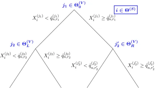
The construction of the individual trees is summarized in the table below and is illustrated in Figure1.

Algorithm 1 Tree construction

1: Parameters: Number of quantiles q, number of subsampled observations an, number of

eligible directions for splitting mtry.

2: Compute the empiricalq-quantiles for each marginal distribution over the whole dataset.

3: Subsample with replacement an observations, indexed byΘ(S). Only these observations

are used to build the tree.

4: Initialize s= 0 (the root of the tree).

5: Draw uniformly at random a subset Θ(sV)⊂ {1, . . . , p} of cardinality mtry.

6: For allj∈Θ(sV), compute the CART-splitting criterion at all empiricalq-quantiles ofX(j)

that split the cell sinto two non-empty cells.

7: Choose the split that maximizes the CART-splitting criterion.

i∈Θ(S) j1 ∈Θ(0V) X(j1) i <qˆ (j1) n,r1 X (j1) i ≥qˆ (j1) n,r1 j2 ∈Θ(_LV) X(j2) i <qˆ (j2) n,r2 X (j2) i ≥qˆ (j2) n,r2 j₂0 ∈Θ(_RV) X(j 0 2) i <qˆ (j0 2) n,r0₂ X (j0 2) i ≥qˆ (j0 2) n,r0₂

Figure 1: Schematic view of a randomized tree of depth 2. Θ(₀V)(resp.,Θ_L(V)and Θ(_RV)) is the set of

coordinates selected to split the root node (resp., its left and right children).

In our context of binary classication, where the output Y ∈ {0,1}, maximizing the

so-called empirical CART-splitting criterion is equivalent to maximizing the criterion based on Gini impurity (see, e.g., Biau and Scornet, 2016). More precisely, at node H and for a cut performed along thej-th coordinate at the empiricalr-thq-quantile qˆn,r(j), this criterion reads:

Ln(H,qˆn,r(j)) def = 1 Nn(H) n X i=1 (Yi−YH)21Xi∈H − 1 Nn(H) n X i=1 Yi−YHL1_X(j) i <qˆ (j) n,r−YHR1Xi(j)≥ˆq (j) n,r 2 1Xi∈H, (2.2)

whereYH is the average of the Yi's such that Xi ∈H, Nn(H) is the number of data points

Xi falling intoH, and

HLdef= {x∈H:x(j)<qˆ(n,rj)} and HRdef= {x∈H :x(j) ≥qˆn,r(j)}.

Note that, for the ease of reading, (2.2) is dened for a tree built with the entire dataset Dn

without resampling.

Following the construction of Algorithm1, SIRUS growsMrandomized trees, where the ex-tra randomness used to build the`-th tree is denoted byΘ`. The random variablesΘ1, . . . ,ΘM

are generated as i.i.d. copies of the generic variableΘ = (Θ(S),Θ(₀V),Θ(_LV),Θ(_RV)), so that tree

structures are independent conditional on the datasetDn.

Path representation In order to go further in the presentation of SIRUS, we still need to introduce a useful notation, which describes the paths that go from the root of the tree to a given node. To this aim, we follow the example shown in Figure 2 with a tree of depth

x(1) x(2) ˆ q_n,(1)₇ ˆ q_n,(1)₅ ˆ q_n,(2)₄ P5 ={(2,4, R), (1,7, L)} P6 ={(2,4, R), (1,7, R)} P3 ={(2,4, L), (1,5, L)} P4={(2,4, L), (1,5, R)} X_i(2)<qˆ(2)_n,4 X_i(2)≥qˆ_n,(2)₄ P1 P2 X_i(1)<qˆ(1)_n,7 X_i(1) ≥qˆ(1)_n,7 P5 P6 X_i(1)<qˆ_n,(1)₅ X_i(1) ≥qˆ(1)_n,5 P3 P4

Figure 2: Example of a root node R2 _{partitionned by a randomized tree of depth 2: the tree on the} right side, the associated paths and hyperrectangles of lengthd= 2on the left side.

document. For instance, let us consider the node P6 dened by the sequence of two splits

X_i(2) ≥ qˆ_n,(2)₄ and X_i(1) ≥ qˆ(1)_n,7. The rst split is symbolized by the triplet (2,4, R), whose

components respectively stand for the variable index2, the quantile index4, and the right side

Rof the split. Similarly, for the second split we cut coordinate 1 at quantile index 7, and pass to the right. Thus, the path to the considered node is dened byP6={(2,4, R),(1,7, R)}. Of

course, this generalizes to each pathP of lengthd= 1 or d= 2 under the symbolic compact

form

P={(jk, rk, sk), k= 1, . . . , d},

where, fork∈ {1, . . . , d}(d∈ {1,2}), the triplet(jk, rk, sk) describes how to move from level

(k−1)to levelk, with a split using the coordinatejk ∈ {1, . . . , p}, the indexrk ∈ {1, . . . , q−1}

of the corresponding quantile, and a sidesk=Lif we go the the left andsk =Rif we go to the

right. The set of all possible such paths is denoted byΠ. It is important to note thatΠis in

fact a deterministic (that is, non random) quantity, which only depends upon the dimensionp and the orderq of the quantilesan easy calculation shows thatΠis a nite set of cardinality 2p(q−1) +p(4p−1)(q−1)2. On the other hand, a Θ-random tree of depth 2 generates (at

most)6 paths inΠ, one for each internal and terminal nodes. In the sequel, we letT(Θ,Dn)

be the list of such extracted paths, which is therefore a random subset of Π. Note that, in

very specic cases, we can have less than6 paths inT(Θ,Dn), typically if one of the two child

nodes does not have any possible splits in the selected directions.

Elementary rule Of course, given a pathP ∈Π one can recover the hyperrectangle (i.e.,

the tree node)_Hˆ_{n associated with P and the entire datasetDn via the correspondence} ˆ Hn(P) = ( x∈_Rp : ( x(jk)_<qˆ(jk) n,rk if sk=L x(jk)_≥qˆ(jk) n,rk if sk=R , k= 1, . . . , d ) . (2.3)

Thus, for each pathP∈Π, we logically dene the companion elementary rule ˆgn,P by ∀x∈_Rp, gˆn,P(x) =    1 Nn( ˆHn(P)) Pn i=1Yi1_Xi∈_Hˆ_n(P) if x∈Hˆn(P) 1 n−Nn( ˆHn(P)) Pn i=1Yi1_Xi∈_/Hˆ_n(P) otherwise,

with the convention0/0 = 0. For x∈_Rp_{, the elementary rule ˆg}

n,P(x) is an estimate of the

probability that x is of class 1, depending whether x falls in _Hˆ_{n(P) or not. We note that}

such a rule depends on the datasetDn and the particular pathP. One small word of caution:

here, the term rule does not stand for classication rule but, as is traditional in the rule learning literature, to a piecewise constant estimate that can take two dierent values and simply reads if conditions on x, then response, else default response.

The elementary rules ˆgn,P will serve as building blocks for SIRUS, which will learn from

a collection of such rules. Since eachΘ-random tree generates (at most) 6 rules through the

path extraction, we can then generate a wide collection of rules using our modied random forest. The next subsection describes how we select and aggregate the most important rules of the forest to form a compact, stable, and predictive rule ensemble model.

2.2 SIRUS

Rule selection Using our modied random forest algorithm, we are able to generate a large numberM of trees (typicallyM = 10 000), randomized byΘ1, . . . ,ΘM. Since we are interested

in selecting the most important rules, i.e., those which represent strong patterns between the inputs and the output, we select rules that are shared by a large portion of trees. As described above, for each Θ`-random tree, we extract 6 rules through the associated paths. To make

this selection procedure explicit, we letpn(P)be the probability that aΘ-random tree of the

forest contains a particular pathP∈Π, that is,

pn(P) =P(P∈T(Θ,Dn)|Dn).

The Monte-Carlo estimate pˆM,n(P) of pn(P), which can be directly computed using the

random forest, takes the form

ˆ pM,n(P) = 1 M M X `=1 1P∈T(Θ`,Dn).

Clearly, pˆM,n(P) is a good estimate of pn(P) when M is large since, by the law of large

numbers, conditional onDn,

lim

M→∞pˆM,n(P) =pn(P) a.s.

We also see thatpˆM,n(P) is unbiased sinceE[ˆpM,n(P)|Dn] =pn(P).

Now, let p0 ∈ (0,1) be a xed parameter to be selected later on. As a general strategy,

in the forest and only retain those that occur with a frequency larger than p0. We are thus

interested in the set

ˆ

PM,n,p0 ={P ∈Π : ˆpM,n(P)> p0}. (2.4)

We see that ifM is large enough, then PˆM,n,p0 is a good estimate of Pn,p0 ={P ∈Π :pn(P)> p0}.

By construction, there is some redundancy in the list of rules generated by the set of distinct paths_Pˆ_M,n,p

0. The hyperrectangles associated with the6 paths extracted from a Θ-random

tree overlap, and so the corresponding rules are linearly dependent. Therefore a post-treatment to lter _Pˆ_M,n,p

0 is needed to make the method operational. The general idea is

straightfor-ward: if the rule associated with the path P ∈ Pˆ_M,n,p0 is a linear combination of rules

associated with paths with a higher frequency in the forest, thenP is removed from_Pˆ_M,n,p

0.

The post-treatment mechanism is fully described and illustrated in AppendixA. Note that the theoretical properties of SIRUS will only be stated for_Pˆ_M,n,p

0 without post-treatment.

How-ever, since the post-treatment is deterministic, all subsequent results still hold when_Pˆ_M,n,p

0

is post-treated (except the second part of Theorem2see Remark 1).

Rule aggregation Recall that our objective is to estimate the conditional probabilityη(x) =

P(Y = 1|X=x) with a few simple and stable rules. To reach this goal, we propose to simply

average the set of elementary rules{gˆn,P :P∈PˆM,n,p0} that have been selected in the rst

step of SIRUS. The aggregated estimateηˆM,n,p0(x) of η(x)is thus dened by

ˆ ηM,n,p0(x) = 1 |Pˆ_M,n,p0| X P∈PˆM,n,p₀ ˆ gn,P(x). (2.5)

Finally, the classication procedure assigns class 1 to an input x if the aggregated estimate ˆ

ηM,n,p0(x)is above a given threshold, and class0otherwise. In the introduction, we presented

an example of a list of 6 rules for the SECOM dataset. In this case, for a new input x, ˆ

ηM,n,p0(x) is simply the average of the outputpf over the 6 selected rules.

In past works on rule ensemble models, such as RuleFit (Friedman et al.,2008) and Node harvest (Meinshausen,2010), rules are also extracted from a tree ensemble, and then combined together through a regularized linear model. In our case, it happens that the parameter p0

alone is enough to control sparsity. Indeed, in our experiments, we observe that adding such linear model in our aggregation method hardly increases the accuracy and hardly reduces the size of the nal rule set, while it can signicantly reduce stability, add a set of coecients that makes the model less straightforward to interpret, and requires more intensive computations. We refer to the experiments in AppendixAfor a comparison betweenηˆM,n,p0 dened as simple

average (2.5) and dened with a logistic regression.

3 Theoretical properties

The construction of the rule ensemble model essentially relies on the path selection and on the estimatespˆM,n(P),P∈Π. Therefore, our theoretical analysis rst focuses on the asymptotic

properties of those estimates in Theorem 1. Among the three minimum requirements for interpretability dened in Section 1, simplicity and predictivity are quite easily met for rule models (Cohen and Singer,1999;Meinshausen,2010;Letham et al.,2015). On the other hand, asLetham et al. (2015) recall, building a stable rule ensemble is challenging. In the second part of the section, we provide a denition of stability in the context of rule models, introduce relevant metrics, and prove the asymptotic stability of SIRUS.

Let us start by dening all theoretical counterparts of the empirical quantities involved in SIRUS, which do not depend on Dn but only on the unknown distribution PX,Y of (X, Y).

For a given integerq≥2 and r∈ {1, . . . , q−1}, the theoretical q-quantiles are dened by q?_r(j) =infx∈_R:P(X(j)≤x)≥ r

q ,

i.e., the population version of qˆ(n,rj) dened in (2.1). Similarly, for a given hyperrectangle

H⊆Rp_{, we let the theoretical CART-splitting criterion be}

L?(H, q?_r(j)) =V[Y|X∈H]

−_P(X(j)< q_r?(j)|X∈H)×_V[Y|X(j)< q_r?(j),X∈H]

−_P(X(j)≥q_r?(j)|X∈H)×_V[Y|X(j)≥q_r?(j),X∈H].

Based on this criterion, we denote byT?(Θ) the list of all paths contained in the theoretical

tree built with randomness Θ, where splits are chosen to maximize the theoretical criterion

L? instead of the empirical one Ln, dened in (2.2). We stress again that the listT?(Θ) does

not depend uponDn but only upon the unknown distribution of(X, Y). Next, we letp?(P)

be the theoretical counterpart ofpn(P), that is

p?(P) =P(P ∈T?(Θ)), and nally dene the theoretical set of selected pathsP?

p0 by {P ∈Π : p

?_{(P) > p}

0} (with

the same post-treatment as for the empirical proceduresee Section 2). Notice that, in the case where multiple splits have the same value of the theoretical CART-splitting criterion, one is randomly selected.

As it is often the case in the theoretical analysis of random forests, we assume through-out this section that the subsampling of an observations to build each tree is done without

replacement to alleviate the mathematical analysis. Note however that Theorem2is valid for subsampling with or without replacement.

3.1 Consistency of the path selection

Our consistency results hold under conditions on the subsampling rateanand the number of

treesMn, together with some assumptions on the distribution of the random vector X. They

are given below.

(A1) The subsampling rate an satises lim

n→∞an=∞ andnlim→∞

an

n = 0.

(A2) The number of trees Mn satises lim

(A3) X has a strictly positive density f with respect to the Lebesgue measure. Furthermore, for all j ∈ {1, . . . , p}, the marginal density f(j) of X(j) is continuous, bounded, and strictly positive.

We are now in a position to state the main result of this section.

Theorem 1. If Assumptions (A1)-(A3) are satised, then, for allP ∈Π, we have lim

n→∞pˆMn,n(P) =p

?_{(P) in probability.}

The proof of Theorem 1 is to be found in the Supplementary Material A. It is however interesting to give a sketch of the proof here. The consistency is obtained by showing that

ˆ

pMn,n(P)is asymptotically unbiased with a null variance. The result for the variance is quite

straightforward since the variance of pˆMn,n(P) can be broken into two terms: the variance

generated by the Monte-Carlo randomization, which goes to0as the number of trees increases

(Assumption (A2)), and the variance ofpn(P). Following Mentch and Hooker(2016), since

pn(P)is a bagged estimate it can be seen as an innite-order U-statistic, and a classic bound

on the variance of U-statistics gives that V[pn(P)] converges to 0 if lim n→∞

an

n = 0, which is

true by Assumption (A1). Next, proving that pˆMn,n(P) is asymptotically unbiased requires

to dive into the internal mechanisms of the random forest algorithm. To do this, we have to show that the CART-splitting criterion is consistent (Lemma 3) and asymptotically normal (Lemma 4) when cuts are limited to empirical quantiles (estimated on the same dataset) and the number of trees grows with n. When cuts are performed on the theoretical quantiles, the law of large numbers and the central limit theorem can be directly applied, so that the proof of Lemmas 3 and 4 boils down to showing that the dierence between the empirical CART-splitting criterion evaluated at empirical and theoretical quantiles converges to 0 in

probability fast enough. This is done in Lemma 2 thanks to Assumption (A3).

The only source of randomness in the selection of the rules lies in the estimatespˆMn,n(P).

Since Theorem1 states the consistency of such an estimation, the path selection consistency follows, as formalized in Corollary1, for all threshold valuesp0 that do not belong to the nite

set U? _{= {p}?_{(P) : P ∈ Π} of all theoretical probabilities of appearance for each path P.}

Indeed, ifp0 =p?(P)for someP ∈Π, thenP(ˆpMn,n(P)> p0) does not necessarily converge

to0 and the path selection can be inconsistent.

Corollary 1. Assume that Assumptions (A1)-(A3) are satised. Then, providedp0 ∈[0,1]\

U?_{, we have}

lim

n→∞P( ˆPMn,n,p0 6=P

? p0) = 0.

Proof of Corollary1. The result is a consequence of Theorem 1since

P PˆMn,n,p0 6=P ? p0 ≤ X P∈Π P(ˆpMn,n(P)> p0)1p?(P)≤p0 +P(ˆpMn,n(P)≤p0)1p?(P)>p0.

Corollary 1 is a stability result, and thus a rst step towards our objective of designing a stable rule ensemble algorithm. However, such an asymptotic result does not guarantee stability for nite samples. Metrics to quantify stability in that case are introduced in the next subsection.

3.2 Stability

In the statistical learning theory, stability refers to the stability of predictions (e.g., Vapnik, 1998). In particular, Rogers and Wagner (1978),Devroye and Wagner (1979), and Bousquet and Elissee(2002) show that stability and predictive accuracy are closely connected. In our case, we are more concerned by the stability of the internal structure of the model, and, to our knowledge, no general denition exists. So, we state the following tentative denition: a rule learning algorithm is stable if two independent estimations based on two independent samples result in two similar lists of rules. Thus, given a new sampleD0

n independent ofDn,

we denepˆ0_M,n(P) and the corresponding set of pathsPˆ_M,n,p0

0 based on a modied random

forest drawn with a parameter Θ0 independent of Θ. We take advantage of a dissimilarity

measure between two sets, the so-called Dice-Sorensen index, often used to assess the stability of variable selection methods (Chao et al.,2006;Zucknick et al.,2008;Boulesteix and Slawski, 2009;He and Yu,2010;Alelyani et al.,2011). This index is dened by

ˆ SM,n,p0 = 2Pˆ_M,n,p0 ∩Pˆ_M,n,p0 0 Pˆ_M,n,p0 + Pˆ_M,n,p0 0 (3.1) with the convention 0

0 = 1. This is a measure of stability taking values between 0 and 1: if the intersection between PˆM,n,p0 and Pˆ

0 M,n,p0 is empty, then ˆ SM,n,p0 = 0, while if ˆ PM,n,p0 = Pˆ 0

M,n,p0, then SˆM,n,p0 = 1. We also dene Sn,p0, the population counterpart of

ˆ SM,n,p0 based on Pn,p0 and P 0 n,p0, as Sn,p0 = 2P_n,p0 ∩P0_n,p0 P_n,p0 + P0_n,p0 . (3.2)

SIRUS is stable regarding the metrics (3.1) and (3.2), as stated in the following corollary. Corollary 2. Assume that Assumptions (A1)-(A3) are satised. Then, providedp0 ∈[0,1]\

U?_{, we have}

lim

n→∞ ˆ

SMn,n,p0 = 1 in probability.

The same limiting result holds forSn,p0.

Proof of Corollary2. We have

ˆ SMn,n,p0 = 2 P P∈Π1pˆMn,n(P)>p0∩ˆp 0 Mn,n(P)>p0 P P∈Π1pˆMn,n(P)>p0 +1pˆ0 Mn,n(P)>p0 .

Sincep0 ∈ U/ ?, we deduce from Theorem 1 and the continuous mapping theorem that, for all P∈Π, lim n→∞1pˆMn,n(P)>p0 =1p?(P)>p0 in probability. Therefore, lim n→∞ ˆ

SMn,n,p0 = 1 in probability. The caseSn,p0 is similar.

Corollary2 shows that the rule ensemble is asymptotically stable for both the innite and nite forests, respectively corresponding to Sn,p0 and SˆMn,n,p0. Of course, the latter case is

of greater interest since only a nite forest is grown in practice. Nevertheless, an important stability requirement for SIRUS is to output the same set of rules when tted multiple times on the same datasetDn, for a xed sample sizenand a givenp0. This means that, conditionally

onDnand withDn0 =Dn,SˆM,n,p0 should be close to1. The rst statement of Theorem2below

shows that this is indeed the case. Theorem2 also provides an asymptotic approximation of

E[ ˆSM,n,p0|Dn]for large values of the number of trees M, which quanties the inuence of M

on the mean stability, conditional onDn. We let Un

def

= {pn(P) : P ∈ Π} be the empirical

counterpart ofU?_.

Theorem 2. Ifp0 ∈[0,1]\ Un andDn0 =Dn, then, conditional onDn, we have

lim

M→∞ ˆ

SM,n,p0 = 1 in probability. (3.3)

In addition, for allp0<max Un,

1−_E[ ˆSM,n,p0|Dn] ∼ M→∞ X P∈Π Φ(M p0, M, pn(P))(1−Φ M p0, M, pn(P))) 1 2 P P0_∈Π1_pn(P0_)>p 0 +1_pn(P0_)>p 0−ρn(P,P0)σn(P 0₎ σn(P)(p0−pn(P)) ,

whereΦ(M p0, M, pn(P))is the cdf of a binomial distribution with parameterpn(P),M trials,

evaluated at M p0, and, for allP,P0 ∈Π,

σn(P) = p pn(P)(1−pn(P)), and ρn(P,P0) = Cov(1P∈T(Θ,Dn),1P0∈T(Θ,Dn)|Dn) σn(P)σn(P0) .

The proof of Theorem 2 is to be found in the Supplementary MaterialA. Despite its ap-parent complexity, the asymptotic approximation of1−E[ ˆSM,n,p0|Dn]can be easily estimated,

and plays an essential role to stop the growing of the forest at an optimal number of treesM, as illustrated in the next section.

Remark 1. As mentioned in Section2, the equivalent provided in Theorem2 is dened when the sets of rules _Pˆ_M,n,p

0 and Pˆ

0

M,n,p0 are not post-treated. It considerably simplies the

analysis of the asymptotic behavior ofE[ ˆSM,n,p0|Dn]. Since the post-treatment is deterministic,

this operation is not an additional source of instability. Then, if the estimation of the rule set without post-treatment is stable, it is also the case when the post-treatment is added. Therefore an ecient stopping criterion for the number of trees can be derived from Theorem 2.

4 Tuning and experiments

We recall that our objective is to design simple, stable, and predictive rule models, with an acceptable computational cost. In practice, for a nite sample Dn, SIRUS relies on two

hyperparameters: the number of treesM and the selection thresholdp0. This section provides

a procedure to set optimal values forM andp0, and illustrates the good performance of SIRUS

on real datasets.

4.1 Tuning of SIRUS

Throughout this section, we should keep in mind that in SIRUS, the random forest is only involved in the selection of the paths. Conditionally onDn, the set of selected pathsPˆM,n,p0 =

{P ∈Π : ˆpM,n(P)> p0} is a good estimate of its population counterpartPn,p0 when M is

large.

Tuning of M to maximize stability As explained in Section 3, an important stability requirement is that SIRUS outputs the same set of rules when tted multiple times on a given datasetDn. This is quantied by the mean stabilityE[ ˆSM,n,p0|Dn], which measures the

expected proportion of rules shared by two ts of SIRUS onDn, for xedn (sample size),p0

(threshold), and M (number of trees). Since the computational cost increases linearly with M, we propose to stop the growing of the forest when the mean stability is close enough to

1, with typically a gap smaller than α = 0.05. Thus, the stopping criterion takes the form 1−_E[ ˆSM,n,p0|Dn]< α.

There are two obstacles to operationalize this stopping criterion: its estimation and its dependence to p0. We make two approximations to overcome these limitations and give

em-pirical evidence of their good practical behavior. First, Theorem 2 provides an asymptotic equivalent of1−_E[ ˆSM,n,p0|Dn], that we simply estimate by

εM,n,p0 = P P∈ΠΦ(M p0, M,pˆM,n(P))(1−Φ(M p0, M,pˆM,n(P))) P P∈Π(1−Φ(M p0, M,pˆM,n(P))) .

Secondly,εM,n,p0 depends on p0, whose optimal value is unknown in the rst step of SIRUS,

when trees are grown. It turns out however that εM,n,p0 is not very sensitive to p0, as shown

by the experiments of Figure7in AppendixA. Consequently, our strategy is to simply average εM,n,p0 over a setVˆM,n of many possible values ofp0 (see AppendixAfor a precise denition)

and use the resulting average as a gauge. Thus, in the experiments, we utilize the following criterion to stop the growing of the forest, with typicallyα= 0.05:

argmin M n 1 |VˆM,n| X p0∈VˆM,n εM,n,p0 < α o . (4.1)

Experiments showing the good empirical performance of this criterion are presented in Ap-pendixA.

Remark 2. We emphasize that growing more trees does not improve predictive accuracy or stability with respect to data perturbation for a xed sample size n. Indeed, the instability of the rule selection is generated by the variance of the estimatespˆM,n(P),P∈Π. Upon noting

that we have two sources of randomnessΘ and Dn, the law of total variance shows that

V[ˆpM,n(P)] can be broken down into two terms: the variance generated by the Monte Carlo

randomnessΘon the one hand, and the sampling variance on the other hand. In fact, equation

(1.3) in the proof of Theorem1 (Supplementary MaterialA) reveals that

V[ˆpM,n(P)] =

1

ME[pn(P)](1−E[pn(P)]) + (1−

1

M)V[pn(P)].

The stopping criterion (4.1) ensures that the rst term becomes negligible asM → ∞, so that

V[ˆpM,n(P)]reduces to the sampling varianceV[pn(P)], which is independent ofM. Therefore,

stability with respect to data perturbation cannot be further improved by increasing the number of trees. Additionally, the trees are only involved in the selection of the paths. For a given set of paths _Pˆ_M,n,p

0, the construction of the nal aggregated estimate ηˆM,n,p0 (see (2.5)) is

independent of the forest. Thus, if further increasing the number of trees does not impact the path selection, neither it improves the predictive accuracy.

Tuning ofp0 to maximize accuracy The parameterp0 is a threshold involved in the

def-inition of_Pˆ_M,n,p

0 to lter the most important rules, and therefore determines the complexity

of the model. The parameterp0 should be set to optimize a tradeo between the number of

rules, stability, and accuracy. In practice, it is dicult to settle such a criterion, and we choose to optimizep0 to maximize the predictive accuracy with the smallest possible set of rules. To

achieve this goal, we proceed as follows. The 1-AUC is estimated by10-fold cross-validation

for a ne grid ofp0values, dened such that|PˆM,n,p0|varies from1to25rules. (We let25be

an arbitrary upper bound on the maximum number of rules, considering that a bigger set is not readable anymore.) The randomization introduced by the partition of the dataset in the

10 folds of the cross-validation process has a signicant impact on the variability of the size

of the nal model. Therefore, in order to get a robust estimation ofp0, the cross-validation is

repeated multiple times (typically30) and results are averaged. The standard deviation of the

mean of 1-AUC is computed over these repetitions for eachp0 of the grid search. We consider

that all models within 2 standard deviations of the minimum of 1-AUC are not signicantly

less predictive than the optimal one. Thus, among these models, the one with the smallest number of rules is selected, i.e., the optimalp0 is shifted towards higher values to reduce the

model size without decreasing predictivitysee Figures3 and4 for examples.

4.2 Experiments

We have conducted experiments on 9 diverse public datasets from the UCI repository (Dua

and Gra,2017; data is described in Table1), as well as on the SECOM data, collected from a semi-conductor manufacturing process. The rst batch of experiments aims at illustrating the good behavior of SIRUS in various settings. Especially, we observe that the restrictions in the forest growing (cut values on quantiles and a tree depth of two) are not strong limitations, and that SIRUS provides a substantial improvement of stability compared to state-of-the-art rule algorithms. On the other hand, the SECOM dataset is an example of a manufacturing process

problem. Typically, data is unbalanced (since most of the production is valid), hundreds of parameters are collected along the production line, with many noisy ones, and the order of interaction between these parameters is low.

Dataset Sample size Total number_{of variables categorical variables}Number of

Haberman 306 3 0 Diabetes 768 8 0 Heart Statlog 270 13 6 Liver Disorders 345 6 0 Heart C2 303 13 8 Heart H2 294 13 7 Credit German 1000 20 13 Credit Approval 690 15 9 Ionosphere 351 33 0

Table 1: Description of UCI datasets

We use the R/C++ software implementation sirus (available from CRAN), adapted from ranger, a fast random forest implementation (Wright and Ziegler,2017). The hyperparameters M andp0 are tuned as explained earlier, we set mtry=bp₃cand q= 10quantiles. Bootstrap

is used for the resampling mechanism, i.e., resampling is done with replacement andan=n.

Finally, categorical variables are transformed in multiple binary variables.

Performance metrics As we have seen several times, an interpretable classier is based on three essential features: simplicity, stability, and predictive accuracy. We introduce rele-vant metrics to assess those properties in the experiments. By denition, the size (i.e., the simplicity) of the rule ensemble is the number of selected rules, i.e., |PˆM,n,p0|. To measure

the predictive accuracy, 1-AUC is used and estimated by10-fold cross-validation (repeated30

times for robustness). With respect to stability, an independent dataset is not available for real data to compute_Sˆ_M,n,p

0 as dened in Corollary2in Subsection3.2. Nonetheless, we can

take advantage of the cross-validation process to compute a stability metric: the proportion of rules shared by two models built during the cross-validation, averaged over all possible pairs. UCI datasets Now, SIRUS is run on the 9 selected UCI datasets. Figure 3 provides an

example for the dataset Credit German of the dependence between predictivity and the number of rules whenp0 varies. In that case, the minimum of 1-AUC is about0.26for SIRUS, 0.21 for Breiman's forests, and 0.31 for CART tree. For the chosen p0, SIRUS returns a

compact set of 18 rules and its stability is 0.66, i.e., about 12 rules are consistent between

two dierent models built in a10-fold cross-validation. Thus, the nal model is simple (a set

of only 18 rules), is quite robust to data perturbation, and has a predictive accuracy close

to random forests. Figure4 provides another example of the good practical performance of SIRUS with the Heart Statlog dataset. Here, the predictivity of random forests is reached with11rules, with a stability of0.69.

Figure 3: For the UCI dataset Credit German, 1-AUC (on the left) and stability (on the right) versus the number of rules whenp0varies, estimated via 10-fold cross-validation (results are averaged over30repetitions).

Figure 4: For the UCI dataset Heart Statlog, 1-AUC (on the left) and stability (on the right) versus the number of rules whenp0 varies, estimated via 10-fold cross-validation (results are averaged over

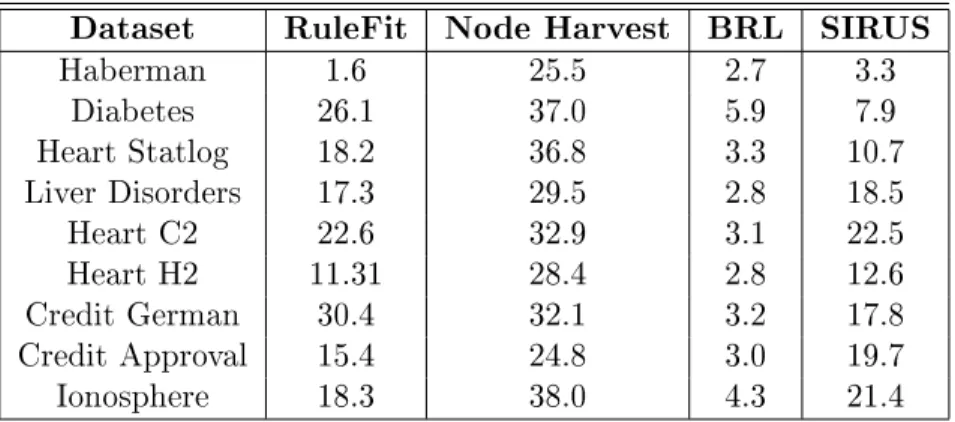
Dataset RuleFit Node Harvest BRL SIRUS Haberman 1.6 25.5 2.7 3.3 Diabetes 26.1 37.0 5.9 7.9 Heart Statlog 18.2 36.8 3.3 10.7 Liver Disorders 17.3 29.5 2.8 18.5 Heart C2 22.6 32.9 3.1 22.5 Heart H2 11.31 28.4 2.8 12.6 Credit German 30.4 32.1 3.2 17.8 Credit Approval 15.4 24.8 3.0 19.7 Ionosphere 18.3 38.0 4.3 21.4

Table 2: Mean model size over a10-fold cross-validation for UCI datasets. Results are averaged over 30repetitions of the cross-validation. (Standard deviations are negligible, they are not displayed to

increase readability.)

Dataset RuleFit Node Harvest BRL SIRUS Haberman 0.57 0.35 0.71 0.65 Diabetes 0.21 0.38 0.80 0.79 Heart Statlog 0.18 0.31 0.34 0.69 Liver Disorders 0.19 0.31 0.48 0.57 Heart C2 0.28 0.53 0.66 0.66 Heart H2 0.23 0.37 0.61 0.65 Credit German 0.12 0.46 0.33 0.66 Credit Approval 0.17 0.26 0.32 0.66 Ionosphere 0.06 0.25 0.78 0.63

Table 3: Mean stability over a 10-fold cross-validation for UCI datasets. Results are averaged over 30repetitions of the cross-validation. (Standard deviations are negligible, they are not displayed to

increase readability. Values within 10% of the maximum are displayed in bold.)

We also evaluated main competitors: CART, RuleFit, Node harvest, and BRL, using available R implementations, respectively rpart (Therneau et al.,2018), pre (Fokkema,2017), nodeharvest (Meinshausen, 2015), and sbrl (Yang et al., 2017). All algorithms were run with their default settings (CART trees are pruned, RuleFit is limited to rule predictors). To compare stability of the dierent methods, data is binned with 10-quantiles, so that the possible rules are the same for all algorithms, and the same stability metric is used. Experimental results are gathered in Table2 for model size, Table3 for stability, and Table4for predictive accuracy.

Clearly, SIRUS is more stable than its competitors. We see that BRL exhibits a comparable stability for a few datasets and generates shorter set of rules, but at the price of a weaker predictive accuracy. RuleFit and Node harvest have a slightly better predictive accuracy than SIRUS, but they are unstable and generate longer sets of rules. Overall, the general conclusion of this rst batch of experiments is that SIRUS improves stability with a predictive accuracy comparable to state-of-the-art methods.

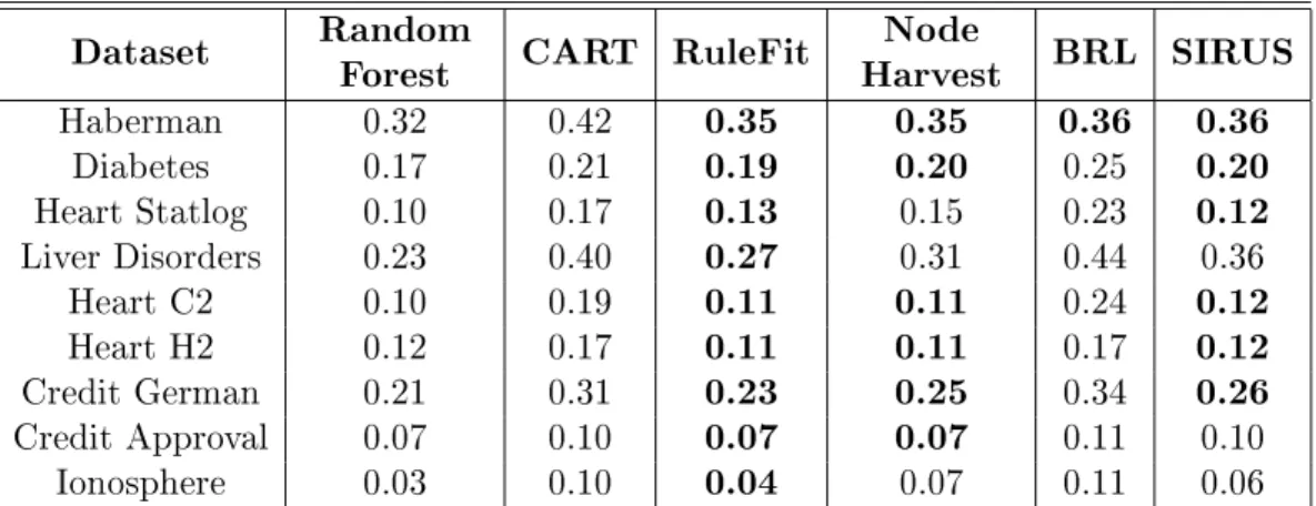
Dataset Random_Forest CART RuleFit _HarvestNode BRL SIRUS Haberman 0.32 0.42 0.35 0.35 0.36 0.36 Diabetes 0.17 0.21 0.19 0.20 0.25 0.20 Heart Statlog 0.10 0.17 0.13 0.15 0.23 0.12 Liver Disorders 0.23 0.40 0.27 0.31 0.44 0.36 Heart C2 0.10 0.19 0.11 0.11 0.24 0.12 Heart H2 0.12 0.17 0.11 0.11 0.17 0.12 Credit German 0.21 0.31 0.23 0.25 0.34 0.26 Credit Approval 0.07 0.10 0.07 0.07 0.11 0.10 Ionosphere 0.03 0.10 0.04 0.07 0.11 0.06

Table 4: Model error (1-AUC) over a10-fold cross-validation for UCI datasets. Results are averaged

over30repetitions of the cross-validation. (Standard deviations are negligible, they are not displayed

to increase readability. Values within 10% of the maximum are displayed in bold.)

Manufacturing process data In this second batch of experiments, SIRUS is run on a real manufacturing process of semi-conductors, the SECOM dataset (Dua and Gra, 2017). Data is collected from sensors and process measurement points to monitor the production line, resulting in590numeric variables. Each of the1567data points represents a single production

entity associated with a label pass/fail (0/1) for in-house line testing. As it is always the case

for a production process, the dataset is unbalanced and contains 104fails, i.e., a failure rate

pf of 6.6%. We proceed to a simple pre-processing of the data: missing values (about 5% of

the total) are replaced by the median. The thresholdp0 and the number of trees are tuned as

previously explained.

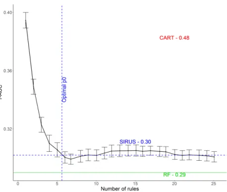
Figure5displays predictivity versus the number of rules whenp0varies. The 1-AUC value

is 0.30 for SIRUS (for the optimal p0 = 0.04), 0.29 for Breiman's random forests, and 0.48

for a pruned CART tree. Thus, in that case, CART tree predicts no better than the random classier, whereas SIRUS has a similar accuracy to random forests. The nal model has 6

rules and a stability of 0.74, i.e., in average 4 to 5 rules are shared by 2 models built in a

10-fold cross-validation process, simulating data perturbation. By comparison, Node harvest outputs34 rules with a value of0.31 for 1-AUC.

Finally, the output of SIRUS may be displayed in the simple and interpretable form of Figure 6. Such a rule model enables to catch immediately how the most relevant variables impact failures. Among the 590 variables, 5 are enough to build a model as predictive as

random forests, and such a selection is quite robust. Other rules alone may also be informative, but they do not add additional information to the model, since predictive accuracy is already minimal with the 6 selected rules. Then, production engineers should rst focus on those 6

Figure 5: For the SECOM dataset, accuracy versus the number of rules whenp0varies, estimated via 10-fold cross-validation (averaged over30repetitions of the cross-validation).

A Additional experiments and settings

This appendix species computational settings and provides additional experiments on the nine UCI datasets used in Section4see Table1.

Rule set post-treatment As explained in Section2, there is some redundancy in the list of rules generated by the set of distinct paths_Pˆ_M,n,p

0, and a post-treatment to lterPˆM,n,p0

is needed to make the method operational. The general principle is straightforward: if the rule associated with the pathP ∈Pˆ_M,n,p0 is a linear combination of rules associated to paths

with a higher frequency in the forest, thenP is removed from _Pˆ_M,n,p

0.

To illustrate the post-treatment, let the tree of Figure 2 be theΘ1-random tree grown in

the forest. Since the paths of the rst level of the tree,P1 and P2, always occur in the same

trees, we have pˆM,n(P1) = ˆpM,n(P2). If we assume these quantities to be greater than p0,

then P1 and P2 belong to PˆM,n,p0. However, by construction, P1 and P2 are associated

with the same rule, and we therefore enforce SIRUS to keep onlyP1 inPˆM,n,p0. Each of the

paths of the second level of the tree,P3,P4,P5, andP6, can occur in many dierent trees,

and their associatedpˆM,n are distinct (except in very specic cases). Assume for example that

ˆ

pM,n(P1) > pˆM,n(P4) > pˆM,n(P5) > pˆM,n(P3) > pˆM,n(P6) > p0. Since gˆn,P3 is a linear

combination ofˆgn,P4 andgˆn,P1,P3 is removed. Similarly P6 is redundant withP1 andP5,

and it is therefore removed. Finally, among the six paths of the tree, onlyP1,P4, and P5

are kept in the list_Pˆ_M,n,p

0.

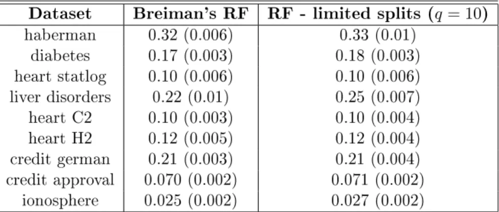
Random forest accuracy As described in Section2, in the forest construction of SIRUS, the splits at each node of each tree are limited to the empiricalq-quantiles of each component of X. We then rst check that this modication alone of the forest has little impact on its accuracy. Using the R package ranger, 1-AUC is estimated for each dataset with 10 fold-cross-validation for q = 10. Results are averaged over 10 repetitions of the cross-validationthe

standard deviation is displayed in parentheses in Table5.

Dataset Breiman's RF RF - limited splits (q = 10)

haberman 0.32 (0.006) 0.33 (0.01) diabetes 0.17 (0.003) 0.18 (0.003) heart statlog 0.10 (0.006) 0.10 (0.006) liver disorders 0.22 (0.01) 0.25 (0.007) heart C2 0.10 (0.003) 0.10 (0.004) heart H2 0.12 (0.005) 0.12 (0.004) credit german 0.21 (0.003) 0.21 (0.004) credit approval 0.070 (0.002) 0.071 (0.002) ionosphere 0.025 (0.002) 0.027 (0.002)

Table 5: Accuracy, measured by 1-AUC (standard deviation) on UCI datasets, for two algorithms: Breiman's random forests and random forests with splits limited to 10-quantiles.

Dataset Mean stability Haberman 0.950 (0.01) Diabetes 0.950 (0.007) Heart Statlog 0.954 (0.007) Liver Disorders 0.951 (0.006) Heart C2 0.955 (0.009) Heart H2 0.952 (0.009) Credit German 0.950 (0.008) Credit Approval 0.941 (0.02) Ionosphere 0.950 (0.009) Table 6: Values of_Sˆ

M,n,p0 averaged over p0 ∈VˆM,n when the stopping criterion (4.1) is used to set

M, for UCI datasets. Results are averaged over10repetitions and standard deviations are displayed

in parentheses.

Denition of _Vˆ_{M,n To design the stopping criterion (4.1) of the number of trees, εM,n,p}

0

is averaged across a set _Vˆ_{M,n of diverse p0 values. These p0 values are chosen to scan all}

possible path sets _Pˆ_M,n,p

0, of size ranging from 1 to 50 paths. When a set of 50 paths is

post-treated, its size reduces to around 25 paths. Thus, as explained in Section 4, 25 is an

arbitrarily threshold on the maximum number of rules above which a rule model is not readable anymore. In order to generate path sets of such sizes, p0 values are chosen halfway between

two distinct consecutivepˆM,n(P),P∈Π, restricted to the highest 50values.

Number of trees We run experiments on the UCI datasets to assess the quality of the stopping criterion (4.1). Recall that the goal of this criterion is to determine the minimum number of trees M ensuring that two independent ts of SIRUS on the same dataset result on two lists of rules with an overlap of 95% in average. This is checked with a rst batch of

experimentssee next paragraph. Secondly, the stopping criterion (4.1) does not consider the optimalp0, unknown when trees are grown in the rst step of SIRUS. Then, another batch of

experiments is run to show that the stability approximation1−εM,n,p0 is quite insensitive to

p0. Finally, a last batch of experiments provides examples of the number of trees grown when

SIRUS is t.

Experiments 1 For each dataset, the following procedure is applied. SIRUS is run a rst time using criterion (4.1) to stop the number of trees. This initial run provides the optimal number of trees M as well as the set VˆM,n of possible p0. Then, SIRUS is t twice

independently using the precomputed number of trees M. For each p0 ∈ VˆM,n, the stability

metric _Sˆ_M,n,p

0 (with D

0

n = Dn) is computed over the two resulting lists of rules. Finally

ˆ

SM,n,p0 is averaged across all p0 values in VˆM,n. This procedure is repeated 10 times: results

are averaged and presented in Table 6, with standard deviations in parentheses. Across the considered datasets, resulting values range from0.941to 0.955, and are thus close to0.95 as

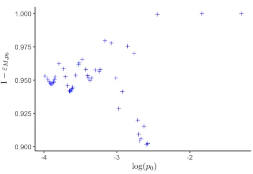
Figure 7: For the UCI dataset Credit German,1−εM,n,p0 for a sequence ofp0∈VˆM,p0corresponding

to nal models ranging from1to about25rules.

Experiments 2 The second type of experiments illustrates thatεM,n,p0 is quite

insensi-tive top0 whenM is set with criterion (4.1). For the Credit German dataset, we t SIRUS

and then compute1−εM,n,p0 for eachp0 ∈VˆM,n. Results are displayed in Figure7. 1−εM,n,p0

ranges from0.90to1, where the extreme values are reached forp0 corresponding to very small

number of rules, which are not of interest whenp0is selected to maximize predictive accuracy.

Thus,1−εM,n,p0 is quite concentrated around 0.95 whenp0 varies.

Experiments 3 Finally, we display in Table 7 the optimal number of trees when the growing of SIRUS is stopped using criterion (4.1). It ranges from 4220 to 20 650 trees. In

Breiman's forests, the number of trees above which the accuracy cannot be signicantly im-proved is typically 10 times lower. However SIRUS grows shallow trees, and is thus not

computationally more demanding than random forests overall.

Logistic regression In Section 2, ηˆM,n,p0(x) (2.5) is a simple average of the set of rules,

dened as ˆ ηM,n,p0(x) = 1 |Pˆ_M,n,p0| X P∈PˆM,n,p0 ˆ gn,P(x). (A.1)

To tackle our binary classication problem, a natural approach would be to use a logistic regression and dene

ln ηˆM,n,p0(x) 1−ηˆM,n,p0(x) = X P∈_Pˆ_M,n,p 0 β_Pˆgn,P(x), (A.2)

Dataset Nb of trees (sd) Haberman 10 920 (877) Diabetes 18 830 (1538) Heart Statlog 7840 (994) Liver Disorders 14 650 (1242) Heart C2 6840 (1270) Heart H2 4220 (529) Credit German 7940 (672) Credit Approval 20 650 (8460) Ionosphere 7320 (487)

Table 7: Number of treesM determined by the stopping criterion (4.1) for UCI datasets. Results are averaged over10repetitions and standard deviations are displayed in parentheses.

Figure 8: For the UCI dataset Credit German, 1-AUC versus the number of rules when p0 varies, estimated via 10-fold cross-validation (repeated30times) for two dierent methods of rule aggregation:

the rule average (A.1) in red and a logistic regression (A.2) in blue.

where the coecientsβ_P have to be estimated. To illustrate the performance of the logistic regression (A.2), we consider again the UCI dataset, Credit German. We augment the previous results from Figure 3 (in Section 4) with the logistic regression error in Figure 8. One can observe that the predictive accuracy is slightly improved but it comes at the price of an additional set of coecients that can be hard to interpret (some can be negative), and an increased computational cost.

Supplementary Material

Proofs of Theorems1and2 are available in Supplementary Material for: SIRUS: Mak-ing random forests interpretable.

References

S. Alelyani, Z. Zhao, and H. Liu. A dilemma in assessing stability of feature selection algo-rithms. In 13th IEEE International Conference on High Performance Computing & Com-munication, pages 701707, Piscataway, 2011. IEEE.

G. Biau and E. Scornet. A random forest guided tour. Test, 25:197227, 2016.

A.-L. Boulesteix and M. Slawski. Stability and aggregation of ranked gene lists. Briengs in Bioinformatics, 10:556568, 2009.

O. Bousquet and A. Elissee. Stability and generalization. Journal of Machine Learning Research, 2:499526, 2002.

L. Breiman. Bagging predictors. Machine Learning, 24:123140, 1996. L. Breiman. Random forests. Machine Learning, 45:532, 2001a.

L. Breiman. Statistical modeling: The two cultures (with comments and a rejoinder by the author). Statistical Science, 16:199231, 2001b.

L. Breiman. Setting up, using, and understanding random forests v3.1. 2003a. URL https: //www.stat.berkeley.edu/~breiman/Using_random_forests_V3.1.pdf.

L. Breiman, J.H. Friedman, R.A. Olshen, and C.J. Stone. Classication and Regression Trees. Chapman & Hall/CRC, Boca Raton, 1984.

A. Chao, R.L. Chazdon, R.K. Colwell, and T.-J. Shen. Abundance-based similarity indices and their estimation when there are unseen species in samples. Biometrics, 62:361371, 2006.

P. Clark and T. Niblett. The cn2 induction algorithm. Machine Learning, 3:261283, 1989. W.W. Cohen. Fast eective rule induction. In Proceedings of the Twelfth International

Con-ference on Machine Learning, pages 115123. Morgan Kaufmann Publishers Inc., San Fran-cisco, 1995.

W.W. Cohen and Y. Singer. A simple, fast, and eective rule learner. In Proceedings of the Sixteenth National Conference on Articial Intelligence and Eleventh Conference on Innovative Applications of Articial Intelligence, pages 335342, Palo Alto, 1999. AAAI Press.

K. Dembczy«ski, W. Kotªowski, and R. Sªowi«ski. Ender: A statistical framework for boosting decision rules. Data Mining and Knowledge Discovery, 21:5290, 2010.

L. Devroye and T. Wagner. Distribution-free inequalities for the deleted and holdout error estimates. IEEE Transactions on Information Theory, 25:202207, 1979.

F. Doshi-Velez and B. Kim. Towards a rigorous science of interpretable machine learning. arXiv:1702.08608, 2017.

Dheeru Dua and Casey Gra. UCI machine learning repository, 2017. URLhttp://archive. ics.uci.edu/ml.

M. Fokkema. Pre: An r package for tting prediction rule ensembles. arXiv:1707.07149, 2017. Eibe Frank and Ian H Witten. Generating accurate rule sets without global optimization. In Proceedings of the Fifteenth International Conference on Machine Learning, pages 144151, San Francisco, 1998. Morgan Kaufmann Publishers Inc.

A.A. Freitas. Comprehensible classication models: A position paper. ACM SIGKDD Explo-rations Newsletter, 15:110, 2014.

J.H. Friedman, B.E. Popescu, et al. Predictive learning via rule ensembles. The Annals of Applied Statistics, 2:916954, 2008.

J. Fürnkranz and G. Widmer. Incremental reduced error pruning. In Proceedings of the 11th International Conference on Machine Learning, pages 7077, San Francisco, 1994. Morgan Kaufmann Publishers Inc.

Z. He and W. Yu. Stable feature selection for biomarker discovery. Computational Biology and Chemistry, 34:215225, 2010.

K. Kumbier, S. Basu, J.B. Brown, S. Celniker, and B. Yu. Rening interaction search through signed iterative random forests. arXiv:1810.07287, 2018.

B. Letham. Statistical learning for decision making: Interpretability, uncertainty, and infer-ence. PhD thesis, Massachusetts Institute of Technology, 2015.

B. Letham, C. Rudin, T.H. McCormick, and D. Madigan. Interpretable classiers using rules and bayesian analysis: Building a better stroke prediction model. The Annals of Applied Statistics, 9:13501371, 2015.

Z.C. Lipton. The mythos of model interpretability. arXiv:1606.03490, 2016.

N. Meinshausen. Node harvest. The Annals of Applied Statistics, 4:20492072, 2010. N. Meinshausen. Package `nodeharvest', 2015.

L. Mentch and G. Hooker. Quantifying uncertainty in random forests via condence intervals and hypothesis tests. Journal of Machine Learning Research, 17:841881, 2016.

R.S. Michalski. On the quasi-minimal solution of the general covering problem. In Proceedings of the Fifth International Symposium on Information Processing, pages 125128, New York, 1969. ACM.

W.J. Murdoch, C. Singh, K. Kumbier, R. Abbasi-Asl, and B. Yu. Interpretable machine learning: Denitions, methods, and applications. arXiv:1901.04592, 2019.

J.R. Quinlan. C4.5: Programs for Machine Learning. Morgan Kaufmann, San Mateo, 1992. M.T. Ribeiro, S. Singh, and C. Guestrin. Why should i trust you? explaining the predictions

of any classier. In Proceedings of the 22nd ACM SIGKDD International Conference on Knowledge Discovery and Data Mining, pages 11351144, New York, 2016. ACM.

R.L. Rivest. Learning decision lists. Machine Learning, 2:229246, 1987.

W.H. Rogers and T.J. Wagner. A nite sample distribution-free performance bound for local discrimination rules. The Annals of Statistics, 6:506514, 1978.

C. Rudin. Please stop explaining black box models for high stakes decisions. arXiv:1811.10154, 2018.

S. Rüping. Learning interpretable models. PhD thesis, Universität Dortmund, 2006. T. Therneau, B. Atkinson, B. Ripley, and Maintainer B. Ripley. Package `rpart', 2018. V. Vapnik. Statistical Learning Theory. 1998, volume 3. Wiley, New York, 1998.

S.M. Weiss and N. Indurkhya. Lightweight rule induction. In Proceedings of the Seventeenth International Conference on Machine Learning, pages 11351142, San Francisco, 2000. Mor-gan Kaufmann Publishers Inc.

Marvin N Wright and Andreas Ziegler. ranger: A fast implementation of random forests for high dimensional data in c++ and r. Journal of Statistical Software, 77:117, 2017.

H. Yang, C. Rudin, and M. Seltzer. Scalable bayesian rule lists. In Proceedings of the 34th International Conference on Machine Learning, volume 70, pages 39213930. Proceedings of Machine Learning Research, 2017.

B. Yu. Stability. Bernoulli, 19:14841500, 2013.

B. Yu and K. Kumbier. Three principles of data science: Predictability, computability, and stability (pcs). arXiv:1901.08152, 2019.

M. Zucknick, S. Richardson, and E.A. Stronach. Comparing the characteristics of gene ex-pression proles derived by univariate and multivariate classication methods. Statistical Applications in Genetics and Molecular Biology, 7:134, 2008.