A Unified Algorithm for Fitting Penalized Models with High Dimensional Data

(1)

A Unified Algorithm for Fitting Penalized Models with

High Dimensional Data

A DISSERTATION

SUBMITTED TO THE FACULTY OF THE GRADUATE SCHOOL OF THE UNIVERSITY OF MINNESOTA

BY

Yi Yang

IN PARTIAL FULFILLMENT OF THE REQUIREMENTS FOR THE DEGREE OF

Doctor of Philosophy

Advisor: Hui Zou

(2)

c

Yi Yang 2013

(3)

Acknowledgements

Writing this Ph.D. thesis would not have been possible without the valuable support of quite a number of persons. First of all I thank my advisor Hui Zou for his immense support, the inspirational meetings and discussions.

Thanks to my colleagues Teng Zhang, Wei Qian, Qing Mai, Yuwen Gu, Zhihua Su and Ying Nan. I very much enjoy working at the department. I am especially grateful to Teng Zhang for giving me tremendous amount of help. I am grateful to the committee members of my thesis, consisting of Yuhong Yang, Glen Meeden and Vipin Kumar, for investing their time to read and evaluate my Ph.D.thesis.

I want to thank my parents, Ling Bai and Xinmin Yang, for supporting my interest in statistics and always encouraging me to do what makes me happy (even though they probably still do not understand how hard science can make anyone happy).

(4)

Dedication

To my parents who nursing me with affections and love and their dedicated partnership for success in my life

(5)

Abstract

In the light of high dimensional problems, research on the penalized model has received much interest. Correspondingly, several algorithms have been developed for solving penalized high dimensional models. In this thesis, we propose fast and efficient unified algorithms for computing the solution path for a collection of penalized models. In particular, we study the algorithm for solving`1 penalized learning problems and the

algorithm for solving group-lasso learning problems. These algorithm take advantage of a majorization-minimization trick to make each update simple and efficient. The algorithms also enjoy a proven convergence property. To demonstrate the generality of our algorithms, we further extend these algorithms on a class of elastic net penalized large margin classification methods and the elastic net penalized Cox’s proportional hazards model. These algorithms have been implemented in three R packages gglasso, gcdnet and fastcox, which are publicly available from the Comprehensive R Archive Network (CRAN) at http://cran.r-project.org/web/packages. On simulated and real data, our algorithms consistently outperform the existing software in speed for computing penalized models and often delivers better quality solutions.

(6)

List of Tables

2.1 Timings of glmnetand glmnet2 for some simulated data 1 . . . 16

2.2 Timings of glmnetand glmnet2 for some simulated data 2 . . . 17

2.3 Timings (in seconds) of glmnetand glmnet2 for some real data . . . . 18

3.1 The QM condition . . . 31

3.2 The FHT model scenario 1 timing . . . 40

3.3 The FHT model scenario 1 KKT condition check . . . 42

3.4 Real Datasets . . . 43

3.5 Group-lasso penalized regression and classification on real datasets . . . 45

4.1 Timings forWZZ and hubernet for simulated data 1 . . . 66

4.2 Timings forWZZ and hubernet for simulated data 2 . . . 67

4.3 Timings forWZZ and hubernet for some real data . . . 68

4.4 Timings for the elastic net penalized classification methods . . . 69

4.5 Testing error and timings for some real data . . . 70

5.1 Timings forcoxnetand cocktail 1 . . . 80

5.2 Timings forcoxnetand cocktail 2 . . . 81

5.3 KKT condition check forcoxnetand cocktail 1 . . . 83

5.4 KKT condition check forcoxnetand cocktail 2 . . . 84

5.5 Timings and KKT check forcoxnetand cocktailfor a real data . . . . 86

(10)

List of Figures

2.1 The running time of glmnet2 for computing solution paths . . . 19 2.2 The CMD algorithm for the ordinary least squares problem . . . 22 3.1 A sparse additive logistic regression model using the group-lasso . . . . 27 3.2 The FHT model scenario 2 timing . . . 41 3.3 Compare the lasso and the group-lasso on Sonar data . . . 46 4.1 Solution paths and timings of the HHSVM on the prostate cancer data . 50 4.2 Loss functions of the classification methods . . . 52 4.3 The first derivative of the loss functions of the classification methods . . 62 5.1 Solution paths and timings on the lung cancer data . . . 85 6.1 Penalty functions . . . 90

(11)

Chapter 1

Introduction

1.1 Background

With the advances in modern technology, high-dimensional data frequently appear in fields such as medical and biological sciences, finances and economics, etc. The maxi-mum partial likelihood estimator does not work well in the presence of high-dimensional covariates. Sparse penalized model offer a way to conduct continuous subset selection while address the overfitting issue for high dimensional problems in which the number of variables is much larger than the number of observations. In sparse penalized models many variables with zero coefficient estimates are automatically deleted, while nonzero coefficients left indicate the important variables. With sparsity, model selection can improve estimation accuracy as well as model interpretability.

There has been great amount of research work contributed in sparse penalized mod-els. In some special models, solution path is piece-wise linear, for example: Least Angle Regression (LARS) for the lasso [1]. LARS-EN for the elastic net [2]. LARS-SVM for`1 -penalized SVM (Zhuet al., 2003). LARS for piecewise quadratic Loss+piecewise linear penalty (or vice versa) [3]. For some other important models, their solution paths are curved. Important examples include: `1-penalized logistic regression/Cox’s regression.

Algorithms were also developed for computing curved `1 solution paths: [4] and [5]

use the connection between Boosting algorithm and the lasso method. [6] proposed the predictor-corrector method of convex-optimization for computing solution path. [7] proposes a generalized Lars algorithm with the loss function approximated by a

(12)

quadratic spline.

Coordinate-wised optimization method works extremely well in solving penalized models. [8] proposed the shooting algorithm. [9] extended shooting for the lasso pe-nalized logistic regression. [10] developed coordinate descent algorithms for the lasso penalized regression, also [11] [12] [13] developed the elastic net penalized GLMs where they used CD loop within a Newton-Ralphson loop for efficiently solving the solution path. The computational efficiency of coordinate descent is due to the fast speed to carry out a simple update on each coordinate; and taking advantage of the sparsity -many of the coefficients remains zero thus the algorithm can skip them and focus on updating the non-zeros, which saves tremendous computing time.

Here we propose a new unified algorithm called coordinate majorization descent (CMD) for computing the solution path for a collection of penalized models. The CMD has the advantages of CD. In addition, the CMD at some points resembles MM algorithms [14][15]. Thus CMD shares the virtue of MM algorithm [16]: (a) providing the convergence of CMD by the descent property of MM algorithms [17]. (b) avoiding large matrix inversions like one did in Newton-Raphson methods. (c) turning a non-differentiable problem into a smooth problem. Given certain conditions hold, it always guarantees convergence to the global solution of convex problems [18] and a local solution of non-convex problems. Most importantly it works for much larger class of penalized models. The possible loss functions can be the following:

• Least Squares

• Logistic regression

• Cox proportional hazards partial likelihood

• Squared SVM

• Huber loss for classification [19]

The penalty function in the model can be one of the following:

• Lasso [20] / Adaptive lasso [21]

• Elastic net [2] / Generalized elastic net [22]

(13)

3

1.2 A short introduction to sparse penalized models

The inputs we have are:

• A training data X = (x1, . . . ,xn)|, y = (y1, . . . , yn)|, where xi ∈ Rp and for

regression yi ∈R, for two-class classificationy∈ {±1}.

• The design matrix X= (xij) is standardized so that each column has mean 0 and variance 1.

• A convex nonnegative loss functionalL:Rn×Rn→R.

• A nonnegative penalty functionalP :Rp→R, withp(0) = 0.

Consider estimating a sparse vector of coefficients β based on training data, through penalized empirical loss minimization

ˆ

β(λ) = argmin

β∈Rp

[L(y,Xβ) +λP(β)] (1.1) whereλ >0 is the regularization parameter;λ= 0 corresponds to no regularization and limλ→∞βˆ(λ) = 0. One often need to compute the solution at a fine grid ofλ’s in

order to pick a data-driven optimal λfor fitting a ’best’ final model.

P(β) is a sparsity-inducing penalty to produce a sparse estimator, which is especially preferred when pn. Some widely used regularization methods include the lasso, the elastic net and the grouped lasso penalty.

The lasso [20] is a very popular technique for high-dimensional modeling

λP(β) =λ||β||1.

Lasso yields sparse estimates ofβbecause it shrinks small lease squares estimates ˆβ_jols’s toward exact zero. [24] proposed the elastic net penalty as an improved variant of the lasso for high-dimensional data when predictors are highly correlated. It connects the lasso penalty and the ridge penalty

λP(β) =λ||β||₁+1

2λ2||β||2 (λ2 >0).

The group-lasso [23] is a generalization of the lasso for doing group-wise variable selec-tion. [23] motivated the group-wise variable selection problem. In such cases, one often

(14)

hope that a group of predictors should either be all included or excluded. Suppose that there are K groups and β(k) denotes the coefficients of Xj’s in kth group. Then the group lasso penalty is

λP(β) =λ

K

X

k=1

kβ(k)k₂.

Many “modern” machine learning methods can be cast in the framework of penalized optimization [3]. In penalized regression problems, the loss function takes the form

L(y,Xβ) =X i

l(yi−x|iβ)

where the residuals yi−x|_iβ quantifies the discrepancy between an observationyi and a linear predictor x|_iβ. An example is the lasso penalized least squares:

Least Squares : βˆ(λ) = argmin

β " 1 2n n X i=1 (yi−x|_iβ) +λ||β||1 # In classification problems, L(y,Xβ) =X i l(yix|_iβ)

where (yix|iβ) are margins for classification. Examples are the lasso penalized logistic regression and support vector machine using squared hinge loss or Huberized squared hinge loss with the lasso penalty.

Logistic : βˆ(λ) = argmin β 1 n n X i=1 log 1 +e−yix|iβ +λ||β||1 Squared SVM : βˆ(λ) = argmin β 1 n n X i=1 (1−yix|iβ) 2 ++λ||β||1 Huberized SVM : βˆ(λ) = argmin β 1 n n X i=1 Hc(yix|_iβ) +λ||β||1 whereHc(t) =        0 (1−t)2/2δ 1−t−δ/2 t >1 1−δ < t≤1 t≤1−δ

(15)

5 Another well known example of penalized model is Cox’s partial likelihood. Assume we have ntraining samples (yi,xi, di)in=1 whereyi is the survival time; 1−di is the the censoring indicator: di= 1 indicates no censoring and di = 0 indicates right censoring; Denote by t1 < t2 <· · · < tS the distinct failure times; letRs be the risk set at time

ts−0 and let ks be the index of the failure at time ts (meaning that patient ks died at time ts). Assume (1) noninformative censoring, (2) proportional hazards, then the negative log-partial-likelihood with the lasso regularization is

Cox0s Model βˆ(λ) = argmin

β 1 n S X s=1 −x|_k_sβ+ log   X k∈Rs exp(x|_kβ)  +λ||β||1

1.3 Thesis outline

This thesis consists of four papers to be found in Chapters 2-5.

In Chapter 2, we consider a family of coordinate majorization descent algorithms in-cluding the classical coordinate descent as a special case. The generalization is actually very straightforward. We simply replace each of the coordinate descent step with a co-ordinate majorization descent (CMD) operation and everything else in glmnet stays the same. Numerical experiments show that this simple CMD trick can lead to substantial improvement in speed when the predictors have moderate or high correlations.

In Chapter 3, we formulate the general group-lasso learning problem. We introduce the qudaratic majorization (QM) condition and show that many popular loss functions for regression and classification satisfy the QM condition. We then derive the BMD algorithm for solving the group-lasso model satisfying the QM condition and discuss some important implementation issues. Simulation and real data examples are also presented.

In Chapter 4, we review the HHSVM and then introduce the GCD algorithm for computing the HHSVM. We study the descent property of the GCD algorithm by mak-ing an intimate connection to the MM principle. The analysis motivates us to further consider a generic GCD algorithm for handling a class of elastic net penalized large margin classifiers. Numerical experiments are presented in the end.

(16)

coordinate descent into a new coordinate-majorization-descent algorithm (CMD). We further show how to integrate the strong rule and the CMD algorithm, which leads to the final cocktail algorithm for computing the solution paths of the elastic net penalized Cox’s regression. Numerical examples are presented in the last section.

(17)

Chapter 2

A Coordinate Majorization

Descent Algorithm for

`

₁

Penalized Learning

2.1 Chapter Overview

The glmnet package by [12] is an extremely fast implementation of the standard coor-dinate descent algorithm for solving`1 penalized learning problems. In this chapter, we consider a family of coordinate majorization descent algorithms for solving the`1

penal-ized learning problems by replacing each coordinate descent step with a coordinate-wise majorization descent operation. Numerical experiments show that this simple modifica-tion can lead to substantial improvement in speed when the predictors have moderate or high correlations.

2.2 Introduction

The lasso [20] is a very popular technique for high-dimensional modeling. A key contrib-utor to the tremendous popularity of the lasso is the celebratedLeast Angle Regression

(LARS) algorithm proposed by [1]. LARS efficiently produces the piecewise linear so-lution paths of the lasso penalized least squares with the computational cost of a single

(18)

least squares fit. Another efficient algorithm for solving the lasso is the cyclical coor-dinate descent algorithm. [8] developed the first working coordinate descent algorithm for solving the lasso. Some recent papers have made coordinate descent a popular computational algorithm for sparse regression. See [25], [11], [10], among others.

[2] proposed the elastic net penalty as an improved variant of the lasso to better handle correlated variables and to stabilize the lasso solution paths. The`1 component

of the elastic net is responsible for achieving sparsity. Hence one can regard the elastic net as a member of the `1 penalized methods. [2] developed the LARS-EN algorithm

for computing the entire solution paths of the elastic net penalized least squares. [12] developed the glmnet package to implement a coordinate descent algorithm for fitting the entire lasso or elastic net regularization paths for generalized linear models. Numer-ical experiments in [12] showed that glmnet is faster than the other publicly available packages for solving the `1 penalized models.

2.3 Coordinate Majorization Descent

2.3.1 Review of glmnet

Because we present an improved glmnet algorithm, it is convenient and necessary to review some key elements of glmnet first. Consider the penalized least squares (PLS) problem. Given a training dataset with N observations (xi, yi) where x denotes a p dimensional predictor vector andyis a continuous response. Without loss of generality, let us assume that the predictors are standardized: PN

i=1xij = 0, 1

N

PN

i=1x2ij = 1, for

j = 1, . . . , p. We use a linear functionβ0+x|β to predicty. Define a penalized residual

sum squares as follows

R(β0, β) = 1 2N N X i=1 (yi−β0−x|iβ)2+Pλ,α(β), (2.1)

where Pλ,α(β) is the elastic net penalty [2] and it is defined as

Pλ,α(β) =λPjp=1pα(βj) = λ p X j=1 1 2(1−α)β 2 j +α|βj| . (2.2)

Then the fitted model is obtained via ( ˆβ,β0ˆ ) = argmin

(β0,β)∈Rp+1

R(β0, β).The elastic net with

(19)

9 Algorithm 1 The coordinate descent algorithm for the elastic net PLS

1. Initialize ( ˜β0,β˜).

2. Cyclic coordinate descent, for j= 1,2, . . . , p: compute ri =yi−β0˜ −x|_iβ˜ and

ˆ βj = S_N1 PN i=1xijri+ ˜βj, λα 1 +λ(1−α) . 3. Set ˜βj = ˆβj.

4. Repeat steps 2−3 until convergence of ˆβ.

α <1 yields better prediction accuracy.

For each fixedλ, cyclic coordinate descent can be easily implemented for solving the elastic net. To keep our discussion concise, we refer interested readers to [12] for more details. We just discuss the main ideas. Let ri =yi−β˜0−x|iβ˜be the current residual. To update the estimate for βj we need to solve a univariate elastic net problem

ˆ βj = argmin βj R(βj|β0,˜ β˜), (2.3) where R(βj|β˜0,β˜) = 1 2 βj−β˜j 2 − 1 N N X i=1 rixij βj−β˜j +λpα(βj). (2.4)

It turns out that (2.3) has a simple closed form solution [2]

ˆ βj = S 1 N PN i=1xijri+ ˜βj, λα 1 +λ(1−α) , (2.5)

whereS(z, t) = (|z|−t)+sgn(z). We next set ˜βj = ˆβj as the new estimate. The operation is sequentially conducted on each coordinate βj till convergence. See Algorithm 1.

(20)

Algorithm 2 The CMD algorithm for the elastic net PLS 1. Initialize ( ˜β0,β˜).

ˆ β_jB = S_N1 PN i=1xijri+f·β˜j, λα f ·1 +λ(1−α) . (f ≥1) 3. Set ˜βj = ˆβjB.

2.3.2 The majorization trick

We now introduce a family of generalized coordinate descent algorithms. We consider modifying the update formula (2.5) as follows

ˆ β_jB= S_N1 PN i=1xijri+f·β˜j, λα f·1 +λ(1−α) (f ≥1) (2.6)

and hence Algorithm 1 becomes Algorithm 2.

Comparing (2.5) and (2.6), one can see that the generalization lies in an extra constant factor f. Whenf = 1, (2.6) reduces to (2.5). We will show that as long as f

is greater or equal to 1, Algorithm 2 is guaranteed to converge. We have verified that with f = 1 glmnet2 and glmnet not only give exactly identical solutions but also use the same timing. Interestingly, when using some f greater than 1, Algorithm 2 can enjoy faster convergence than Algorithm 1. In numerical experiments presented in this chapter we set f = 2 unless stated otherwise.

The convergence property of Algorithm 1 comes from the fact that each operation by (2.5) minimizes the objective function along the jth coordinate direction, which is the basic idea of coordinate descent. We show that each operation by (2.6) at least decreases the objective function along the jth coordinate direction if f > 1. To appreciate this fact, we invoke the Majorization-Minimization (MM) principle [17, 16, 26] which can be regarded as a more generalized form of the famous Expectation-Maximization algorithm [14].

(21)

11 To apply the MM principle, define

Q(βj) = 1 2f· βj −β˜j 2 − 1 N N X i=1 rixij βj−β˜j +λpα(βj). (2.7)

Note that ˆβ_jB actually minimizesQ(βj), i.e.,

ˆ

β_jB= argmin βj

Q(βj). (2.8)

On the other hand, we have

Q(βj)−R(βj|β0,˜ β˜) = 1

2(f −1)(βj− ˜

βj)2. (2.9)

Therefore, for any f >1,Q(βj)> R(βj|β˜0,β˜) unlessβj = ˜βj. Hence we have

R( ˆβ_jB|β˜0,β˜) = Q( ˆβjB) +R( ˆβjB|β˜0,β˜)−Q( ˆβjB) (2.10)

≤ Q( ˜βj) (2.11)

= R( ˜βj|β0,˜ β˜). (2.12)

Obviously,R( ˆβ_jB|β0,˜ β˜) =R( ˜βj|β0,˜ β˜) if and only if ˆβBj = ˜βj. The above arguments show that Algorithm 2 retains the essential descent property of the original coordinate descent algorithm. So it is a genuine coordinate-wise descent algorithm. Because the MM principle is crucial to its descent property, Algorithm 2 is named coordinate majorization descent algorithm.

Unlike Algorithm 1, Algorithm 2 does not take the steepest descent step along each coordinate direction. This seems counterintuitive, as we usually want to decrease the objective function as much as we can at each iteration. In fact, when the predictors are uncorrelated, Algorithm 1 gives the exact solution after one cycle, while Algorithm 2 still needs to iterate. Thus we expect to see Algorithm 1 is faster than Algorithm 2 when the predictors are uncorrelated or nearly uncorrelated. However, in high dimensional data the predictors often have strong correlations or many moderate correlations. What we have found is that in such more complex situations Algorithm 2 can be substantially faster than Algorithm 1. In Section 3.4 we offer some explanation to this interesting phenomenon.

(22)

Algorithm 3 The coordinate descent algorithm for the elastic net PWLS 1. Initialize ( ˜β0,β˜).

ˆ βj = S_N1 PN i=1ωixijri+ 1 N PN i=1ωix2ij ˜ βj, λα 1 N PN i=1ωix2ij+λ(1−α) . (2.14) 3. Set ˜βj = ˆβj.

2.3.3 Penalized weighted least squares and logistic regression

Often we need to assign a weight ωi (other than 1/N) to each observation in least squares. For example, weighted least squares handles linear regression with heteroscades-tic variance and iterative weighted least squares is a classical algorithm for fitting many statistical models. Both Algorithm 1 and Algorithm 2 can be easily modified to deal with the elastic net penalized weighted least squares (PWLS) in which the objective function is min (β0,β)∈Rp+1 1 2N N X i=1 ωi(yi−β0−x|iβ) 2₊_P λ,α(β). (2.13)

Algorithm 3 computes that the solution to (2.13) [12]. Following the arguments in Section 2.2 we derive a coordinate majorization descent algorithm for solving (2.13). See Algorithm 4.

In a logistic regression model we have a binary response variable Y = {0,1} and assume

Pr(Y = 1|x) = 1

1 + exp (−β0+x|β)

=pi.

We consider the elastic net penalized maximum likelihood estimate

( ˆβ0,βˆ) = argmin (β0,β)∈Rp+1 " −1 N N X i=1 {yilogpi+ (1−yi) log (1−pi)}+Pλ,α(β) # . (2.16)

The un-penalized logistic regression is often solved by using the Newton-Raphson algo-rithm in many standard statistical packages. glmnet uses a similar strategy and it is so

(23)

13 Algorithm 4 The CMD algorithm for the elastic net PWLS

1. Initialize ( ˜β0,β˜).

ˆ βB_j = S_N1 PN i=1ωixijri+f · 1 N PN i=1ωix2ij ˜ βj, λα f· 1 N PN i=1ωix2ij +λ(1−α) . (f >1) (2.15) 3. Set ˜βj = ˆβ_jB.

far the fastest algorithm for computing the elastic net penalized logistic regression with high dimensional data. Basically, glmnet uses coordinate descent within the iterative re-weighted least squares loop to solve the penalized logistic regression problems. Let ( ˜β0,β˜) be the current estimate in the iterative re-weighted least squares. As in the usual

logistic regression, we define the following quantities

ηi = ˜β0+x|iβ,˜ p˜i = 1 1 + exp (−η˜i), zi(˜ηi) = ˜ηi+ yi−p˜i ˜

pi(1−p˜i), ωi(˜ηi) = ˜pi(1−p˜i).

The Newton-Raphson algorithm finds the updated solution by solving

min (β0,β)∈Rp+1 ( 1 2N N X i=1

ωi(˜ηi)(zi(˜ηi)−β0−x|_iβ)2+Pλ,α(β)

)

. (2.17)

Glmnet calls Algorithm 3 to solve (2.17). The complete glmnet algorithm for penalized logistic regression is given in Algorithm 5. Our package glmnet2 is almost identical to glmnet except that we use Algorithm 4 to solve (2.17).

2.4 Numerical Experiments

Glmnet uses several tricks to boost its speed, including pathwise descent, warm start and active set convergence. For the sake of space we do not repeat the details of these

(24)

Algorithm 5 Glmnet and Glmnet2 for penalized logistic regression 1. Initialize ( ˜β0,β˜), and set ˜ηi = ˜β0+x|_iβ˜ fori= 1, . . . , N.

2. Compute zi=zi(˜ηi) and ωi=ωi(˜ηi).

3. Glmnet calls Algorithm 3 and Glmnet 2 calls Algorithm 4 to solve

( ˆβ0,βˆ) = argmin (β0,β)∈Rp+1 1 2N N X i=1 ωi(zi−β0−x|iβ) 2₊_P λ,α(β). 4. Set ˜β = ˆβ,β0˜ = ˆβ0.

tricks here. The readers are referred to [12] for the warn start trick, which deals with initial values for the iterative coordinate descent, and the active set trick. In the latest version of glmnet (version 1.7), glmnet further uses the strong rule trick [27]. In order for us to show that the timing difference between glmnet and glmnet2 is solely due to the extra factor f, we need to make sure that the two algorithms use the same implementation tricks. To do so, we took the coreFortranroutines used in glmnet and added the extra f factor in those used for doing the soft-thresholding operation.

In glmnet version 1.7 the convergence criterion is max j ˆ βold j −βˆjnew 2 < 2_{. The}

same convergence criterion is used in glmnet2. In this section = 10−5. We compare the run times of glmnet and glmnet2. All timings were carried out on an Intel Core 2 Duo 2.4 GHz processor.

2.4.1 Simulated data

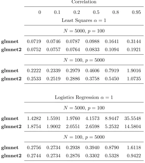
To fix idea, we usef = 2 in this subsection. We further explore the effect off on timing in Section 2.4.3. Consider Friedman’s model for timing comparison [12]. We simulated data with N observations and p predictors where each pair of predictors Xj and Xj0

(25)

15 (N = 5000, p= 100) and (N = 100, p= 5000). The response variable was generated by

Y =

p

X

j=1

Xjβj+k·N(0,1),

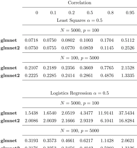
where βj = (−1)jexp(−(2j −1)/20) and k is set to make the signal-to-noise ratio equal 3. For logistic regression, we used the same simulation setup as above, except we define p= 1/(1 + exp(−Y)) and generate a two class response Y0 is generated with Pr(Y0 = 0) =p Pr(Y0= +1) = 1−p. For each data set we computed its elastic net solution paths with α= 1 andα= 0.5 for 100λvalues. In Table 2.1 and 2.2 We report the average run time of glmnet and glmnet2 over 10 independent runs.

2.4.2 Real data

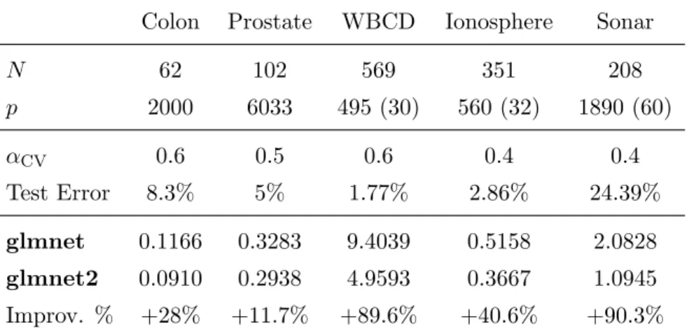
We also compared glmnet and glmnet2 on some benchmark data sets. See Table 2.3. Colon [28] and Prostate [29] are the typical examples of the pN data. In the other three data sets, Wisconsin Breast Cancer Diagnostic (WBCD) data; Ionosphere data and Sonar data [30], the original dimension is less than the sample size. We expanded the predictor set by including the second order polynomials and pairwise interactions of the original predictors. Then the expanded dimension becomes much larger or at least similar to the sample size; see row 2 of Table 2.3. We fit the elastic net penalized logistic regression model on each data set and used 10-fold cross-validation to chooseα; see row 3 of Table 2.3. Fix α = αCV. We compared the running time of glmnet and glmnet2. The relative speed improvement is defined as (tglmnet−tglmnet2)/tglmnet2. We can see than glmnet2 is noticeably faster than glmnet, especially on the WBCD and Sonar.

2.4.3 Exploring the factor size

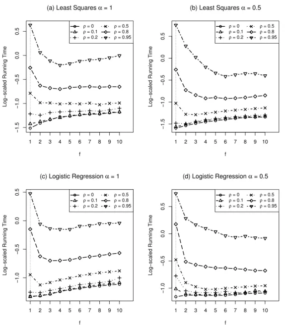
We have fixed f = 2 in the previous numerical examples. Now we further explore the effect of f on timing. In Figure 2.1 we plotted the run time (in log scale) against f for different correlation levels varying from 0 to 0.95. The dotted vertical reference line in each panel indicates the run time of glmnet. We see that when ρ= 0 increasingf only slows down the convergence, which is expected. However, when the correlation becomes stronger (ρ ≥0.2), the curve starts to have a valley and using some f >1 can reduce

(26)

Correlation 0 0.1 0.2 0.5 0.8 0.95 Least Squares α= 1 N = 5000,p= 100 glmnet 0.0719 0.0746 0.0787 0.0988 0.1641 0.3144 glmnet2 0.0752 0.0757 0.0764 0.0833 0.1094 0.1921 N = 100, p= 5000 glmnet 0.2222 0.2339 0.2979 0.4606 0.7919 1.9016 glmnet2 0.2533 0.2519 0.2886 0.3758 0.5450 1.0735 Logistics Regressionα= 1 N = 5000,p= 100 glmnet 1.4282 1.5591 1.9760 4.1573 8.9447 35.5548 glmnet2 1.8754 1.9002 2.0551 2.6598 5.2532 14.5804 N = 100, p= 5000 glmnet 0.2756 0.2734 0.2938 0.3940 0.8790 1.6118 glmnet2 0.2744 0.2734 0.2876 0.3302 0.5328 0.9422

Table 2.1: Timings (in seconds) forglmnetand glmnet2 in the elastic net penalized (α= 1) regression and logistic regression. Total time for 100λvalues, averaged over 10 independent runs.

(27)

17 Correlation 0 0.1 0.2 0.5 0.8 0.95 Least Squares α= 0.5 N = 5000,p= 100 glmnet 0.0718 0.0750 0.0802 0.1003 0.1704 0.5112 glmnet2 0.0750 0.0755 0.0770 0.0859 0.1145 0.2526 N = 100, p= 5000 glmnet 0.2107 0.2189 0.2356 0.3669 0.7765 2.1528 glmnet2 0.2225 0.2285 0.2414 0.2861 0.4876 1.3335 Logistics Regressionα= 0.5 N = 5000,p= 100 glmnet 1.5438 1.6540 2.0519 4.3477 11.9141 37.5434 glmnet2 2.0086 2.0039 2.1666 2.9319 6.1041 16.8284 N = 100, p= 5000 glmnet 0.3193 0.3573 0.4661 0.6217 1.1428 2.0621 glmnet2 0.3176 0.3253 0.3456 0.4042 0.5980 1.3126

Table 2.2: Timings (in seconds) forglmnetand glmnet2 in the elastic net penalized (α= 0.5) regression and logistic regression. Total time for 100 λvalues, averaged over 10 independent runs.

(28)

Colon Prostate WBCD Ionosphere Sonar N 62 102 569 351 208 p 2000 6033 495 (30) 560 (32) 1890 (60) αCV 0.6 0.5 0.6 0.4 0.4 Test Error 8.3% 5% 1.77% 2.86% 24.39% glmnet 0.1166 0.3283 9.4039 0.5158 2.0828 glmnet2 0.0910 0.2938 4.9593 0.3667 1.0945 Improv. % +28% +11.7% +89.6% +40.6% +90.3%

Table 2.3: Timings (in seconds) of glmnet andglmnet2 for some real data, averaged over 10 runs.

the computing time. From Figure 2.1 it seems that 2 is a good default value for f. We also see that when the correlation is very high such as ρ= 0.8 or higher,f = 4 orf = 6 can even work slightly better than f = 2. On the other hand, using f = 4 or f = 6 can have much bigger loss in speed when correlation is low compared to using f = 2. It would be also interesting to decide f’s value based on the empirical correlations. We tested this idea and did not find this strategy works noticeably better than just using

f = 2.

2.4.4 Some explanation of the acceleration effect

We have shown by numerical experiments that using f >1 in the CMD could lead to faster convergence than the ordinary coordinate descent using f = 1, especially when the predictors are highly correlated. Now we attempt to provide some explanation to this acceleration effect. To gain some insight, we consider a simpler case where we use the CMD to solve the ordinary least squares problem with p predictors, defined as ˆβ = argmin β∈_Rp 1 2N y−xβT 2

. This model is a special point on the `1 penalized least squares solution path. Without loss of generality assume all predictors are standardized such that xj = _N1 PNi=1xij = 0, s2xj =

1

N

PN

i=1(xij−xj)2 = 1, for j = 1,· · ·, p. To simplify the analysis, we further assume that the pairwise sample correlation is a constant, i.e., _N1 PN

(29)

19 −1.5 −1.0 −0.5 0.0 0.5

(a) Least Squares α = 1

f

Log−scaled Running Time

1 2 3 4 5 6 7 8 9 10 ρ = 0 ρ = 0.1 ρ = 0.2 ρ = 0.5 ρ = 0.8 ρ = 0.95 −1.5 −1.0 −0.5 0.0 0.5 (b) Least Squares α = 0.5 f

1 2 3 4 5 6 7 8 9 10 ρ = 0 ρ = 0.1 ρ = 0.2 ρ = 0.5 ρ = 0.8 ρ = 0.95 −1.0 −0.5 0.0 0.5 (c) Logistic Regression α = 1 f

1 2 3 4 5 6 7 8 9 10 ρ = 0 ρ = 0.1 ρ = 0.2 ρ = 0.5 ρ = 0.8 ρ = 0.95 −1.0 −0.5 0.0 0.5 (d) Logistic Regression α = 0.5 f

1 2 3 4 5 6 7 8 9 10 ρ = 0 ρ = 0.1 ρ = 0.2 ρ = 0.5 ρ = 0.8 ρ = 0.95

Figure 2.1: The running time of glmnet2 for computing solution paths at 100 λs of the elastic net penalized regression and logistic regression with α = 1 and α = 0.5, averaged over 10 independent runs. The factor size f varies from 1 to 10. The data were generated from the simulation model in Section 2.4.1 with N = 100, p = 5000. Each curve corresponds to a different correlation level.

(30)

Given below is the CMD algorithm for the least squares regression problem:

1. Initialize ˜β =β(0).

2. For k= 1,2,3,· · ·, iterate step 3 until convergence of ˜β.

3. For j = 1,· · ·, p, fix ˜β = (β₁(k),· · · , β(_jk₋)₁, β_j(k−1), β_j(k₊₁−1),· · · , βp(k−1)), we update thej-th coordinate of ˜β, ˜ β(_jk) = argmin βj 1 2f(βj−β (k−1) j ) 2₋ 1 Nx | j y−xβ˜|(βj−β_j(k−1)) (2.18) = β˜(−ρ f,· · · ,− ρ f | {z } j−1 ,1− 1 f,− ρ f,· · ·,− ρ f | {z } p−j )|+x | jy f N. (2.19)

We have used the equal correlation assumption to simplify (18) to get (19). Note that we can rewrite (19) in step 3 as follows

˜ βnew= ˜βWj+υj, (2.20) where ˜ βnew= β₁(k),· · ·, β_j(₋k)₁, β_j(k), β_j(k₊₁−1),· · · , β_p(k−1) , υj = (0,· · ·, x|_jy f N,· · ·,0). Wj =Ip×p+ h 0p×(j−1) uj 0p×(N−j) i , uj = (ukj)p×1 =    −1 f k=j −_fρ k6=j .

Using (2.20), we find that after a complete cycle from j= 1 to j =p we can write

˜ β(k)= ˜β(k−1)A+µ, (2.21) where A= p Y j=1 Wj, µ= p−1 X s=1  υs p Y j=s+1 Wj  +υp. (2.22)

Then by a simple transformation ˜γ(k)= ˜β(k)+ω whereω= (I−A)−1µwe can express (21) in terms of ˜γ(k) and ˜γ(k−1) as follows

(31)

21 which means that

γ(k) =Akγ(0), (2.24) and γ (k) = A k_γ(0) ≤ q ηmax (Ak)|Ak γ (0) , (2.25) where ηmax Ak | Ak

is the maximum eigenvalue of Ak|

Ak.

From (2.25) one can see that the convergence rate of the CMD algorithm for the least squares problem is determined by ηmax Ak

|

Ak

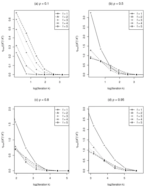
, which is affected by bothf andρ. Although we do not find an explicit expression of ηmax Ak|Ak, we can compute it numerical values easily. We did the calculation for p = 10 and Figure 2.2 displays the calculatedηmax Ak

|

Ak

as a function of log(k) for different combinations of (f, ρ). It is not surprising to see that as k (the number of iterations) increases,ηmax Ak|Ak goes to zero, for all factors considered there. As shown in Figure 2.2 panel (a), when the correlation is low, f = 1 has the fastest convergence. However, when ρ= 0.5 as shown in Figure 2.2 panel (b), f = 2 starts to outperform f = 1. When the correlation is even higher like in Figure 2.2 panels (c) and (d), f = 2,3,4,5 clearly dominatesf = 1.

The above theoretical results are derived for the least squares problem. The analysis is not directly generalized to the more general `1 penalized least squares or logistic

regression. However, the analysis does show us that in using the coordinate decent scheme to solve a multivariate optimization problem, taking the steepest descent in each coordinate direction is not necessarily the best strategy for achieving convergence in the multi-dimension space.

(32)

0.0 0.1 0.2 0.3 0.4 0.5 0.6 (a) ρ = 0.1 log(Iteration k) ηm a x (( A k) TA k) 1 2 3 f = 1 f = 2 f = 3 f = 4 f = 5 0.0 0.5 1.0 1.5 2.0 2.5 3.0 (b) ρ = 0.5 log(Iteration k) ηm a x (( A k) TA k) 1 2 3 f = 1 f = 2 f = 3 f = 4 f = 5 0.0 0.5 1.0 1.5 2.0 (c) ρ = 0.8 log(Iteration k) ηm a x (( A k) TA k) 2 3 4 5 f = 1 f = 2 f = 3 f = 4 f = 5 0.0 0.5 1.0 1.5 2.0 2.5 3.0 (d) ρ = 0.95 log(Iteration k) ηm a x (( A k) TA k) 3 4 5 f = 1 f = 2 f = 3 f = 4 f = 5

Figure 2.2: The CMD algorithm for the ordinary least squares problem with p = 10 predictors. ηmax Ak

|

Ak (as defined in (2.25)) against the number of iterations (in logarithm scale) for 5 different factors (f = 1,2,3,4,5). Each panel corresponds to a different correlation level.

(33)

Chapter 3

A Fast Unified Algorithm for

Group-Lasso Problems

3.1 Chapter Overview

This chapter concerns a class of group-lasso learning problems where the objective function is the sum of an empirical loss and the group-lasso penalty. For a class of loss function satisfying a quadratic majorization condition, we derive a unified algo-rithm called blockwise-majorization-decent (BMD) for efficiently computing the so-lution paths of the corresponding group-lasso penalized learning problem. BMD al-lows for general design matrices, without requiring the predictors to be group-wise orthonormal. As illustration examples, we develop concrete algorithms for solving the group-lasso penalized least squares and several group-lasso penalized large mar-gin classifiers. These group-lasso models have been implemented in an R package gglasso publicly available from the Comprehensive R Archive Network (CRAN) at http://cran.r-project.org/web/packages/gglasso. On simulated and real data, gglasso consistently outperforms the existing software for computing the group-lasso that implements either the classical blockwise descent algorithm or Nestrov’s method.

(34)

3.2 Introduction

The lasso [20] is a very popular technique for variable selection for high-dimensional data. Consider the classical linear regression problem where we have a continuous response y∈ Rn and ann×p design matrix X. The lasso linear regression solves the

following`1 penalized least squares:

argmin β0,β 1 2ky−β0−Xβk 2 2+λ p X j=1 |βj|. (3.1)

The group-lasso [23] is a generalization of the lasso for doing group-wise variable se-lection. [23] motivated the group-wise variable selection problem by two important examples. The first example concerns the multi-factor ANOVA problem where each factor is expressed through a set of dummy variables. In the ANOVA model, deleting an irrelevant factor is equivalent to deleting a group of dummy variables. The second example is the commonly used additive model in which each nonparametric component may be expressed as a linear combination of basis functions of the original variables. Removing a component in the additive model amounts to removing a group of coeffi-cients of the basis functions. In general, suppose that the predictors are put into K

non-overlapping groups such that (1,2, . . . , p) =SK

k=1Ik where the cardinality of index set Ik is pk and IkTIk0 =∅fork6=k0. Consider the linear regression model again and

the group-lasso linear regression model solves the following penalized least squares:

argmin β0,β 1 2ky−β0−Xβk 2 2+λ K X k=1 √ pkkβ(k)k2, (3.2) where kβ(k)k₂ =qP j∈Ikβ 2

j . The group-lasso idea has been used in penalized logistic regression [31].

The group-lasso is computationally more challenging than the lasso. The entire solution paths of the lasso penalized least squares can be efficiently computed by the

least angle regression (LARS) algorithm [1]. See also the homotopy algorithm of [32]. However, the LARS-type algorithm is not applicable to the group-lasso penalized least squares, because its solution paths are not piecewise linear. Another efficient algorithm for solving the lasso problem is the coordinate descent algorithm [18, 8, 33, 34, 35, 36]. [23] implemented a block-wise descent algorithm for the group-lasso penalized

(35)

25 least squares by following the idea of [8]. However, their algorithm requires the group-wise orthonormal condition, i.e., XT

(k)X(k) = Ipk where X(k) = [· · ·Xj· · ·], j ∈ Ik. [31] also developed a block coordinate gradient descent algorithm BCGD for solving the group-lasso penalized logistic regression. Meier’s algorithm is implemented in an R package grplasso available from the Comprehensive R Archive Network (CRAN) athttp://cran.r-project.org/web/packages/grplasso. Later [37] proposed ISTA-BC algorithm, which is an extension of the ISTA/FISTA [38] based on variable step-lengths. The author also pointed out that ISTA-BC can be viewed as a simplified version of the Block Coordinate Descent algorithm.

From an optimization viewpoint, it is more interesting to solve the group-lasso with a general design matrix. From a statistical perspective, the group-wise orthonormal con-dition should not be the basis of a good algorithm for solving the group-lasso problem, even though we can transform the predictors within each group to meet the group-wise orthonormal condition. The reason is that even when the group-wise orthonormal con-dition holds for the observed data, it can be easily violated when removing a fraction of the data or perturbing the dataset as in bootstrap or sub-sampling. In other words, we cannot perform cross-validation, bootstrap or sub-sampling analysis of the group-lasso, if the algorithm’s validity depends on the group-wise orthonormal condition. In a popular MATLAB package SLEP, [39] implemented Nesterov’s method [40, 41] for a variety of sparse learning problems. For the group-lasso case, SLEP provides func-tions for solving the group-lasso penalized least squares and logistic regression. Nes-terov’s method can handle general design matrices. The SLEP package is available at http://www.public.asu.edu/~jye02/Software/SLEP.

In this chapter we consider a general formulation of the group-lasso penalized learn-ing where the learnlearn-ing procedure is defined by minimizlearn-ing the sum of an empirical loss and the group-lasso penalty. The aforementioned group-lasso penalized least squares and logistic regression are two examples of the general formulation. We propose a simple unified algorithm, blockwise-majorization-decent (BMD), for solving the general group-lasso learning problems under the condition that the loss function satisfies a quadratic majorization (QM) condition. BMD is remarkably simple and has provable numerical convergence properties. We show that the QM condition indeed holds for many popular loss functions used in regression and classification, including the squared error loss, the

(36)

Huberized hinge loss, the squared hinge loss and the logistic regression loss. It is also important to point out that BMD works for general design matrices, without requiring the group-wise orthogonal assumption. We have implemented the proposed algorithm in an R package gglassowhich contains the functions for fitting the group-lasso penal-ized least squares, logistic regression, Huberpenal-ized SVM using the Huberpenal-ized hinge loss and squared SVM using the squared hinge loss. The Huberized hinge loss and squared hinge loss are interesting losses functions for classification from machine learning view-point. In fact, there has been both theoretical and empirical evidence showing that the Huberized hinge loss is better than the hinge loss [42, 19]. The group-lasso penalized Huberized SVM and squared SVM are not implemented in grplasso and SLEP. To our best knowledge, gglasso is the first publicly available software for computing the group-lasso penalized Huberized SVM and squared SVM for high-dimensional data.

Here we use breast cancer data [43] to demonstrate the speed advantage ofgglasso overgrplasso andSLEP. This is a binary classification problem wheren= 42 and p= 22,283. We fit a sparse additive logistic regression model using the group-lasso. Each variable contributes an additive component which is expressed by five B-spline basis functions. The group-lasso penalty is imposed on the coefficients of five B-spline basis functions for each variable. Therefore, the corresponding group-lasso logistic regression model has 22,283 groups and each group has 5 coefficients to be estimated. Displayed in Figure 3.1 are three solution path plots produced by grplasso,SLEP and gglasso. We computed the group-lasso solutions at 100λvalues on an Intel Xeon X5560 (Quad-core 2.8 GHz) processor. It took SLEP about 450 and grplasso about 360 seconds to compute the logistic regression paths, while gglasso used only about 10 seconds.

3.3 Group-Lasso Models and The QM Condition

3.3.1 Group-lasso penalized empirical loss

To define a general group-lasso model, we need to use abstract notation. Throughout this chapter we use x to denote the generic predictors which are used to fit the group-lasso model. Note thatxmay not be the original variables in the raw data. For example,

(37)

27 −5.5 −5.0 −4.5 −4.0 −3.5 −3.0 −2 −1 0 1 2

(a) SLEP − Liu et al. (2009) Breast Cancer Data (approximately 450 seconds)

Log Lambda Coefficients −5.5 −5.0 −4.5 −4.0 −3.5 −3.0 −2 −1 0 1 2

(b) grplasso − Meier et al. (2008) Breast Cancer Data (approximately 360 seconds)

Log Lambda Coefficients −5.5 −5.0 −4.5 −4.0 −3.5 −3.0 −2 −1 0 1 2 (c) gglasso − BMD Algorithm Breast Cancer Data (approximately 10 seconds)

Log Lambda

Coefficients

Figure 3.1: Fit a sparse additive logistic regression model using the group-lasso on the breast cancer data [43] with n= 42 patients and 22,283 genes (groups). Each gene’s contribution is modeled by 5 B-Spline basis functions. The solution paths are computed at 100 λvalues. The vertical dotted lines indicate the selectedλ(logλ=−3.73) which selects 8 genes.

(38)

if we use the group-lasso to fit an additive regression model. The original predictors are z1, . . . , zq but we generate x variables by using basis functions of z1, . . . , zq. For instance, x1 = z1, x2 = z₁2, x3 = z3₁, x4 = z2, x5 = z₂2, etc. We assume that the user has defined thexvariables and we only focus on how to compute the group-lasso model defined in terms of the x variables.

Let X be the design matrix with n rows and p columns where n is the sample size of the raw data. If an intercept is used in the model, we let the first column of X be a vector of 1. Assume that the group membership is already defined such that (1,2, . . . , p) = SK

k=1Ik and the cardinality of index set Ik is pk, IkTIk0 = ∅ for

k 6= k0,1 ≤k, k0 ≤ K. Group k contains xj, j ∈ Ik, for 1 ≤k ≤ K. If an intercept is included, then I1 ={1}. Given the group partition, we useβ(k) to denote the segment

of β corresponding to groupk. This notation is used for any p-dimensional vector. Suppose that the statistical model links the predictors to the response variableyvia a linear functionf =βT_{x. Let Φ(}_{y, f}_{) be the loss function used to fit the model. In this} work we primarily focus on statistical methods for regression and binary classification, although our algorithms are developed for a general loss function. For regression, the loss function Φ(y, f) is often defined as Φ(y−f). For binary classification, we use{+1,−1}

to code the class labelyand consider the large margin classifiers where the loss function Φ(y, f) is defined as Φ(yf). We obtained an estimate ofβvia the group-lasso penalized empirical loss formulation defined as follows:

argmin β 1 n n X i=1 τiΦ(yi,βTxi) +λ K X k=1 wkkβ(k)k2, (3.3)

where τi≥0 andwk≥0 for all i, k.

Note that we have included two kinds of weights in the general group-lasso formu-lation. The observation weights τis are introduced in order to cover methods such as weighted regression and weighted large margin classification. The default choice for τi is 1 for alli. We have also included penalty weightswks in order to make a more flexible group-lasso model. The default choice for wk is

√

pk. If we do not want to penalize a group of predictors, simply let the corresponding weight be zero. For example, the intercept is typically not penalized so that w1 = 0. Following the adaptive lasso idea [44], one could define the adaptively weighted group-lasso which often has better esti-mation and variable selection performance than the un-weighted group-lasso [45]. Our

(39)

29 algorithms can easily accommodate both observation and penalty weights.

3.3.2 The QM condition

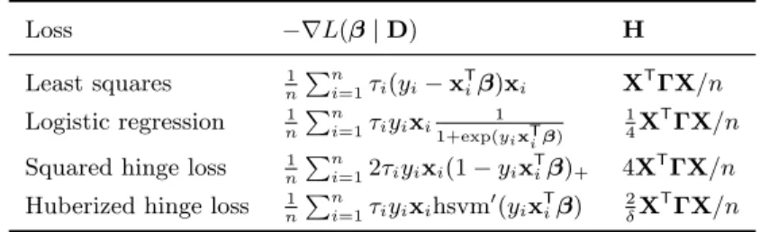
For notation convenience, we use Dto denote the working data{y,X}and letL(β|D) be the empirical loss, i.e.,

L(β|D) = 1 n n X i=1 τiΦ(yi,βTxi).

Definition 1. The loss function Φ is said to satisfy the quadratic majorization (QM) condition, if and only if the following two assumptions hold:

(i). L(β|D) is differentiable as a function of β, i.e., ∇L(β|D) exists everywhere. (ii). There exists a p×p matrix H, which may only depend on the data D, such that

for all β,β∗, L(β|D)≤L(β∗|D) + (β−β∗)T_∇ L(β∗|D) +1 2(β−β ∗ )T H(β−β∗). (3.4) The following lemma characterizes a class of loss functions that satisfty the QM condition.

Lemma 1. Let τi, 1 ≤ i≤ n be the observation weights. Let Γ be a diagonal matrix

withΓii=τi. AssumeΦ(y, f) is differentiable with respect tof and writeΦ0f =

∂Φ(y,f) ∂f . Then ∇L(β|D) = 1 n n X i=1 τiΦ0f(yi,xTiβ)xi.

(1). If Φ0_f is Lipschitz continuous with constant C such that

|Φ0_f(y, f1)−Φ0_f(y, f2)| ≤C|f1−f2| ∀y, f1, f2,

then the QM condition holds for Φ and H= 2_nCXT_ΓX_.

(2). If Φ00_f = ∂Φ_∂f2(y,f2 ) exits and

Φ00_f ≤C2 ∀ y, f,

then the QM condition holds for Φ and H= C2

nX T_ΓX_.

(40)

In what follows we use Lemma 1 to verify that many popular loss functions indeed satisfy the QM condition. The results are summarized in Table 1.

We begin with the classical squared error loss for regression: Φ(y, f) = 1₂(y−f)2.

Then we have ∇L(β|D) =−1 n n X i=1 τi(yi−xTiβ)xi. (3.5) Because Φ00_f = 1, Lemma 1 part (2) tell us that the QM condition holds with

H=XT

ΓX/n≡Hls. (3.6)

We now discuss several margin-based loss functions for binary classification. We code y by {+1,−1}. The logistic regression loss is defined as Φ(y, f) = Logit(yf) = log(1 + exp(−yf)).We have Φ0_f =−y_1+exp(1 _yf₎ and Φ00_f =y2 exp(yf)

(1+exp(yf))2 = exp(yf) (1+exp(yf))2. Then we write ∇L(β|D) =−1 n n X i=1 τiyixi 1 1 + exp(yixTiβ) . (3.7)

Because Φ00_f ≤1/4, by Lemma 1 part (2) the QM condition holds for the logistic regres-sion loss and

H= 1 4X

T

ΓX/n≡Hlogit. (3.8)

The squared hinge loss has the expression Φ(y, f) = sqsvm(yf) = [(1−yf)+]2 where

(1−t)+= ( 0, 1−t, t >1 t≤1.

By direct calculation we have

Φ0_f = ( 0, −2y(1−yf), yf >1 yf ≤1, ∇L(β|D) =−1 n n X i=1 2τiyixi(1−yixTiβ)+. (3.9)

We can also verify that |Φ0_f(y, f1)−Φ0f(y, f2)| ≤ 2|f1−f2|. By Lemma 1 part (1) the

QM condition holds for the squared hinge loss and

(41)

31 Loss −∇L(β|D) H Least squares 1 n Pn i=1τi(yi−xTiβ)xi XTΓX/n Logistic regression 1 n Pn i=1τiyixi 1 1+exp(yixTiβ) 1 4X T_ΓX_/n

Squared hinge loss _n1Pn

i=12τiyixi(1−yix

T

iβ)+ 4XTΓX/n

Huberized hinge loss 1

n

Pn

i=1τiyixihsvm0(yixTiβ) 2δX T_ΓX_/n

Table 3.1: The QM condition is verified for the least squares, logistic regression, squared hinge loss and Huberized hinge loss.

The Huberized hinge loss is defined as Φ(y, f) = hsvm(yf) where

hsvm(t) =        0, (1−t)2/2δ, 1−t−δ/2, t >1 1−δ < t≤1 t≤1−δ.

By direct calculation we have Φ0_f =yhsvm0(yf) where

hsvm0(t) =        0, (1−t)/δ, 1, t >1 1−δ < t≤1 t≤1−δ, ∇L(β|D) =−1 n n X i=1 τiyixihsvm0(yixTiβ). (3.11)

We can also verify that |Φ0_f(y, f1)−Φ0f(y, f2)| ≤ 1_δ|f1−f2|.By Lemma 1 part (1) the

QM condition holds for the Huberized hinge loss and

H= 2 δX T ΓX/n≡Hhsvm. (3.12)

3.4 BMD Algorithm

3.4.1 Derivation

In this section we derive theblockwise-majorization-descent (BMD) algorithm for com-puting the solution of (3.3) when the loss function satisfies the QM condition. The

(42)

objective function is L(β|D) +λ K X k=1 wkkβ(k)k2. (3.13)

Let βe denote the current solution of β. Without loss of generality, let us derive the

BMD update of βe(k), the coefficients of group k. Define H(k) as the sub-matrix of H

corresponding to group k. For example, if group 2 is {2,4} then H2 is a 2×2 matrix

with H(2)₁₁ =H2,2,H(2)12 =H2,4,H(2)21 =H4,2,H(2)22 =H4,4.

Write β such that β(k0) = βe(k

0₎ for k0 6= k. Given β(k0) = βe(k 0₎ for k0 6= k, the optimalβ(k) is defined as argmin β(k) L(β|D) +λwkkβ(k)k2. (3.14)

Unfortunately, there is no closed form solution to (3.14) for a general loss func-tion with general design matrix. We overcome the computafunc-tional obstacle by taking advantage of the QM condition. From (3.4) we have

L(β|D)≤L(βe|D) + (β−βe)T∇L(βe|D) + 1 2(β−βe) T H(β−βe). Write U(βe) =−∇L(βe|D). Using β−βe= (0, . . . ,0 | {z } k−1 ,β(k)−βe(k),0, . . . ,0 | {z } K−k ), we can write L(β|D)≤L(βe|D)−(β(k)−βe(k))TU(k)+ 1 2(β (k)₋ e β(k))T H(k)(β(k)−βe(k)). (3.15)

Next, let γk be the largest eigenvalue of H(k). Thus we can further relax the upper bound in (3.15) as L(β|D)≤L(βe|D)−(β(k)−βe(k))TU(k)+ 1 2γk(β (k)₋ e β(k))T (β(k)−βe(k)). (3.16)

Instead of minimizing (3.14) we solve

argmin β(k) L(βe|D)−(β(k)−βe(k))TU(k)+ 1 2γk(β (k)₋ e β(k))T (β(k)−βe(k)) +λw_kkβ(k)k2. (3.17)

(43)

33 Algorithm 6 The BMD algorithm for general group-lasso learning.

• For k= 1, . . . , K, compute γk, the largest eigenvalue of H(k).

• Initialize βe.

• Repeat the following cyclic blockwise updates until convergence:

– fork= 1, . . . , K, do (1)–(3) ∗ (1) ComputeU(βe) =−∇L(βe|D). ∗ (2) Computeβe(k)(new) = _γ1 k U(k)+γkβe(k) 1− λwk kU(k)₊_γ kβe(k)k2 + . ∗ (3) Setβe(k)=βe(k)(new).

Denote by βe(k)(new) the solution to (3.17). It is straightforward to see that βe(k)(new)

has a simple closed-from expression

e β(k)(new) = 1 γk U(k)+γkβe(k) 1− λwk kU(k)₊_γ kβe(k)k₂ ! + . (3.18)

Algorithm 6 summarizes the details of BMD.

We can prove the decent property of BMD by using the MM principle [46, 16, 47]. Define Q(β|D) =L(βe|D)−(β(k)−βe(k))TU(k)+ 1 2γk(β (k)₋ e β(k))T (β(k)−βe(k)) +λw_kkβ(k)k₂. (3.19) Obviously,Q(β|D) =L(β|D) +λwkkβ(k)k2 when β(k) =βe(k) and (3.16) shows that

forβ(k)6=βe(k),

Q(β|D)> L(β|D) +λwkkβ(k)k2. By the definition of βe(k)(new), we have

L(βe(k)(new)|D) +λw_kkβe(k)(new)k₂ ≤ Q(βe(k)(new)|D) ≤ Q(βe|D)

= L(βe|D) +λw_kkβe(k)k2,

(44)

3.4.2 ISTA-BC with variable stepsizes

After the completion of our work we noticed a unpublished manuscript by [37] where a fast algorithm named ISTA-BC was proposed for solving the group-lasso penalized least squares. It is a block-wise extension of the Iterative Shrinkage Thresholding Algorithm (ISTA) [38]. The critical component of ISTA-BC is that it uses a variable stepsize for each block in the descent operation. The stepsizes are computed using a separate backtracking line-search algorithm [37]. To compare ISTA-BC with BMD, it is necessary to mention details of ISTA-BC first. Recall that the optimization problem of the group-lasso penalized least squares is

argmin β0,β 1 2nky−β0−Xβk 2 2+λ K X k=1 ωkkβ(k)k2,

During the sub-iteration for updating the k-th block, for a chosen stepsizeTk >0, the algorithm considers the following quadratic approximation at the current value of βe(k):

QTk(η (k)_, e β(k)) =g(βe) + (η(k)−βe(k))T∇g(βe) + Tk 2 η (k)₋ e β(k) 2 2+λwk kη(k)k₂, (3.20)

where g(βe) = ₂1_nky−β˜₀−Xβek2₂. We know (3.20) has a closed form minimizer

qTk(βe (k)_{) = argmin} η(k) QTk(η (k)_, e β(k)) = 1 Tk [−∇g(βe)](k)+Tkβe(k) 1− λwk k[−∇g(βe)](k)+Tkβe(k)k2 ! + .

The stepsize is computed using backtracking line-search. It is the smallestTksuch that the following descent condition is satisfied

g(β= [· · ·qTk(βe (k)₎_{· · ·}_{]) +}_λω kkqTk(βe (k)₎_k 2≤QTk(qTk(βe (k)₎_, e β(k)), (3.21) where in (3.21) β = [· · ·qTk(βe (k)₎_{· · ·}_{] has} _β(k0) ₌ e

β(k0) _for _k0 ₆₌ _k_{. Then ISTA-BC}

updates the estimates of the k-th block using βe(k)(new) = q_T

k(βe

(k)_{). The complete}

algorithm of ISTA-BC with backtracking line-search is presented in Algorithm 7. Conceptually, ISTA-BC is a block-wise extension of the ISTA, while BMD is a com-bination of MM principle and block-wise descent. Computationally, ISTA-BC uses back-tracking line search for computing update step-lengths, while BMD’s update is much simpler. Numerically, as will be demonstrated in the next section, BMD is generally faster and more accurate than ISTA-BC.

(45)

35 Algorithm 7 ISTA-BC with backtracking line-search

• Step 0. During the sub-iteration for updating block k, let Tk[0]>0 and a= 2.

• Step m. Repeatedly compute Tk[m]≡aTk[m−1] untilTk satisfies the following condition (3.21).

• Updateβe(k)(new) =q_T_k(βe(k)).

3.4.3 Implementation

We have implemented Algorithm 6 for solving the group-lasso penalized least squares, logistic regression, Huberized SVM and squared SVM. These functions are contained in an R package gglasso publicly available from the Comprehensive R Archive Network (CRAN) athttp://cran.r-project.org/web/packages/gglasso. We always include the intercept term in the model. Without loss of generality we always center the design matrix beforehand.

We solve each group-lasso model for a sequence ofλvalues from large to small. The default number of points is 100. Let λ[l] denote these grid points. We use the warm-start trick to implement the solution path, that is, the computed solution at λ=λ[l] is used as the initial value for using Algorithm 6 to compute the solution at λ=λ[l+ 1]. We define λ[1] as the smallest λ value such that all predictors have zero coefficients, except the intercept. In such a case let ˆβ1 be the optimal solution of the intercept.

Then the solution at λ[1] is βb[1] = ( ˆβ1,0, . . . ,0) as the null model estimates. By the

Karush-Kuhn-Tucker conditions we can find that

λ[1] = max k=1,...,K [∇L(βb[1]|D)] (k) 2/wk, wk 6 = 0.

For least squares and logistic regression models, ˆβ1 has a simple expression:

ˆ β1(LS) = Pn i=1τiyi Pn i=1τi

group-lasso penalized least squares (3.22)

ˆ β1(Logit) = log P yi=1τi P yi=−1τi !

group-lasso penalized logistic regression (3.23)

(46)

1. Initialize ˆβ1 = ˆβ1(Logit) in large margin classifiers.

2. Compute ˆβ1(new) = ˆβ1−_γ1₁∇L(( ˆβ1,0, . . . ,0)|D)1 whereγ1 = 1_nPni=1τi. 3. Let ˆβ1 = ˆβ1(new).

4. Repeat 2-3 until convergence.

For computing the solution at each λwe also utilize the strong rule introduced in [48]. Suppose that we have computed βb(λ[l]), the solution at λ[l]. To compute the

solution at λ[l + 1], before using Algorithm 6 we first check if group k satisfies the following inequality: [∇L(βb(λ[l])|D)] (k) 2 ≥wk(2λ[l+ 1]−λ[l]). (3.24)

Let S ={j :j ∈Ik, group k passes the check in (3.24)}. We use Algorithm 6 to solve the group-lasso model with a reduced data set {y,XS}where XS = [· · ·Xj· · ·], j ∈S corresponds to the design matrix with only the groups of variables in S. Suppose the solution is βb_S. If βb = (βb_S,0) satisfies the KKT condition, then we have found the

desired solution. If not, any group in which there is at least one variable that violates the KKT condition should be added toS, and the procedure continues until Sdoes not change.

In Algorithm 6 we use a simple updating formula to compute ∇L(βe|D), because

it only depends on R = y−Xβe for regression and R = y ·Xβe for classification.

After updatingβe(k), for regression we can updateR byR−X(k)(βe(k)(new)−βe(k)), for

classification update R by R+y·X(k)(βe(k)(new)−βe(k)). In cyclic blockwise descent

updating, we do that on the active-set first which contains those groups whose current coefficients are nonzero. After BMD is converged on the active-set, we then run a complete cycle to see if any group is to be included into the active-set. If not, the algorithm is stopped. Otherwise, BMD is repeated on the updated active-set.

In order to make a fair comparison toISTA-BC,grplassoandSLEP, we tested three different convergence criteria in gglasso:

1. max j |_β˜_j_(current)₋_β˜_j_(new)_| 1+|β˜j(current)| < , forj = 1,2. . . , p. 2. βe(current)−βe(new) 2< .

(47)

37 3. maxk(γk)·max

j

|_β˜_j_(current)−_β˜_j_(new)_|

1+|β˜j(current)| < , forj = 1,2. . . , p and k= 1,2. . . , K. Convergence criterion 1 is used in grplasso and convergence criterion 2 is used in SLEP. We also implemented ISTA-BC algorithm [37] using both criterion 1 (ISTA-BC (LS1)) and 2 (ISTA-BC (LS2)). For the group-lasso penalized least squares and logistic regression, we used both convergence criteria 1 and 2 in gglasso. For the group-lasso penalized Huberized SVM and squared SVM, we used convergence criterion 3 in gglasso. Compared to criterion 1, criterion 3 uses an extra factor maxk(γk) in order to take into account the observation that βe(k)(current)−βe(k)(new) depends on _γ1

k. The default value for is 10−4.

3.5 Numerical Examples

In this section, we use simulation and real data to demonstrate the efficiency of the BMD algorithm in terms of timing performance and solution accuracy. All numerical experiments were carried out on an Intel Xeon X5560 (Quad-core 2.8 GHz) processor. In this section, letgglasso(LS1) andgglasso(LS2) denote the group-lasso penalized least squares solutions computed by gglasso where the convergence criterion is criterion 1 and criterion 2, respectively. Likewise, we definegglasso(Logit1) andgglasso(Logit2) for the group-lasso penalized logistic regression. Similar notation is applied to SLEP, grplasso andISTA-BC.

3.5.1 Timing comparison

We design a simulation model by combining the FHTmodel introduced in [36] and the simulation model 3 in [23]. We generate original predictors Xj, j = 1,2. . . , q from a multivariate normal distribution with a compound symmetry correlation matrix such that the correlation between Xj and Xj0 is ρ forj6=j0. Let

Y∗ = q X j=1 (2 3Xj−X 2 j + 1 3X 3 j)βj,

where βj = (−1)jexp(−(2j −1)/20). When fitting a group-lasso model, we treat

{Xj, Xj2, Xj3} as a group, so the final predictor matrix has the number of variables

(48)

For regression data we generate a response Y = Y∗+k·ewhere the error term e

is generated from N(0,1). k is chosen such that the signal-to-noise ratio is 3.0. For classification data we generate the binary response Y according to

Pr(Y =−1) = 1/(1 + exp(−Y∗)), Pr(Y = +1) = 1/(1 + exp(Y∗)).

We considered the following combinations of (n, p):

Scenario 1. (n, p) = (100,3000) and (n, p) = (300,9000).

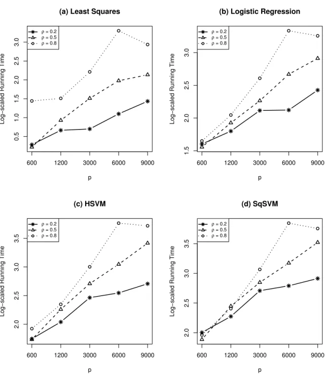
Scenario 2. n= 200 andp= 600,1200,3000,6000,9000, shown in Figure 3.2.

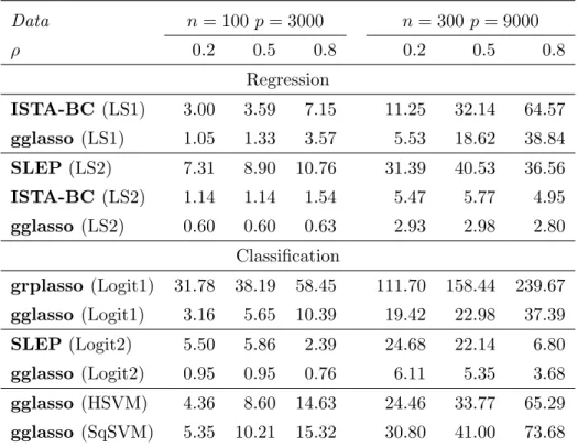
For each (n, p, ρ) combination we recorded the timing (in seconds) of computing the solution paths at 100λvalues of each group-lasso penalized model bygglasso,ISTA-BC, SLEP and grplasso. The results was averaged over 10 independent runs.

Table 3.2 shows results from Scenario 1. We see thatgglasso has the best timing performance. In the group-lasso penalized least squares case, gglasso (LS2) is about 12 times faster than SLEP (LS2) and is about 2 times faster than ISTA-BC (LS2). In the group-lasso penalized logistic regression case, gglasso (Logit2) is about 2-6 times faster thanSLEP(Logit2) andgglasso(Logit1) is about 5-10 times faster thangrplasso (Logit1).

Figure 3.2 shows results from Scenario 2 in which we examine the impact of dimen-sion on the timing of gglasso. We fixednat 200 and plotted the run time (in log scale) against p for three correlation levels 0.2, 0.5 and 0.8. We see that higher ρ increases the timing of gglassoin general. For each fixed correlation level, the timing increases linearly with the dimension.

3.5.2 Quality comparison

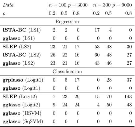
In this section we show that gglasso is also more accurate than ISTA-BC, grplasso and SLEP under the same convergence criterion. We test the accuracy of solutions by checking their KKT conditions. Theoretically, β is the solution of (3.3) if and only if the following KKT conditions hold:

[∇L(β|D)](k)+λwk· β(k) kβ(k)_k 2 =0 ifβ(k)6=0, [∇L(β|D)] (k) 2 ≤λwk ifβ(k)=0,

(49)

39 where k = 1,2, . . . , K. The theoretical solution for the convex optimization problem (3.3) should be unique and always passes the KKT condition check. However, a numer-ical solution could only approach this analytnumer-ical value within certain precision therefore may fail the KKT check. Numerically, we declare β(k) passes the KKT condition check if [∇L(β|D)](k)+λwk· β(k) kβ(k)_k 2 2 ≤ε ifβ(k)6=0, [∇L(β|D)] (k) 2 ≤λwk+ε ifβ(k)=0, for a small ε >0. In this chapter we set ε= 10−4.

For the solutions of the FHT model scenario 1 computed in section 3.5.1, we also calculated the number of coefficients that violated the KKT condition check at each

λ value. Then this number was averaged over the 100 values of λs. This process was then repeated 10 times on 10 independent datasets. As shown in Table 3.3, in the group-lasso penalized least squares case, gglasso (LS1) has zero violation count compared with non-zero violation count of ISTA-BC (LS1); gglasso (LS2) also has smaller violation counts compared with ISTA-BC (LS2) and SLEP (LS2). In the group-lasso penalized classification cases,gglasso(Logit1) has less KKT violation counts than grplasso (Logit1) does when both use convergence criterion 1, and gglasso (Logit2) has less KKT violation counts thanSLEP(Logit2) when both use convergence criterion 2. Overall, it is clear that gglassois numerically more accurate than ISTA-BC,grplasso and SLEP. In addition, gglasso (HSVM) andgglasso (SqSVM) both pass KKT checks without any violation.

3.5.3 Real data analysis

In this section we comparegglasso,ISTA-BC,grplassoand SLEP on several real data examples. Table 5.5 summarizes the datasets used in this section. We fit a sparse

(50)

Timing Comparison Data n= 100 p= 3000 n= 300 p= 9000 ρ 0.2 0.5 0.8 0.2 0.5 0.8 Regression ISTA-BC(LS1) 3.00 3.59 7.15 11.25 32.14 64.57 gglasso (LS1) 1.05 1.33 3.57 5.53 18.62 38.84 SLEP(LS2) 7.31 8.90 10.76 31.39 40.53 36.56 ISTA-BC(LS2) 1.14 1.14 1.54 5.47 5.77 4.95 gglasso (LS2) 0.60 0.60 0.63 2.93 2.98 2.80 Classification grplasso (Logit1) 31.78 38.19 58.45 111.70 158.44 239.67 gglasso (Logit1) 3.16 5.65 10.39 19.42 22.98 37.39 SLEP(Logit2) 5.50 5.86 2.39 24.68 22.14 6.80 gglasso (Logit2) 0.95 0.95 0.76 6.11 5.35 3.68 gglasso (HSVM) 4.36 8.60 14.63 24.46 33.77 65.29 gglasso (SqSVM) 5.35 10.21 15.32 30.80 41.00 73.68

Table 3.2: TheFHTmodel scenario 1. Reported numbers are timings (in seconds) of gglasso,

ISTA-BC,grplassoandSLEPfor computing solution paths at 100λvalues using the

group-lasso penalized least squares, logistics regression, Huberized SVM and squared SVM models. Results are averaged over 10 independent runs.