NBER WORKING PAPER SERIES
ARE CORPORATE DEFAULT PROBABILITIES CONSISTENT WITH THE STATIC TRADEOFF THEORY? Armen Hovakimian Ayla Kayhan Sheridan Titman Working Paper 17290 http://www.nber.org/papers/w17290
NATIONAL BUREAU OF ECONOMIC RESEARCH 1050 Massachusetts Avenue
Cambridge, MA 02138 August 2011
We thank John Graham for providing corporate marginal tax rates data and Shisheng Qu and Erika Jimenez at Moody’s KMV for providing data on their expected default frequency. Financial support from the FDIC Center for Financial Research is gratefully acknowledged. Armen Hovakimian gratefully acknowledges the financial support from the PSC-CUNY Research Foundation of the City University of New York. The Securities and Exchange Commission, as a matter of policy, disclaims responsibility for any private publication or statement by any of its employees. The views expressed herein are those of the author and do not necessarily reflect the views of the Commission, the author’s colleagues upon the staff of the Commission, or the National Bureau of Economic Research.
NBER working papers are circulated for discussion and comment purposes. They have not been peer-reviewed or been subject to the review by the NBER Board of Directors that accompanies official NBER publications.
© 2011 by Armen Hovakimian, Ayla Kayhan, and Sheridan Titman. All rights reserved. Short sections of text, not to exceed two paragraphs, may be quoted without explicit permission provided that full credit, including © notice, is given to the source.
Are Corporate Default Probabilities Consistent with the Static Tradeoff Theory? Armen Hovakimian, Ayla Kayhan, and Sheridan Titman
NBER Working Paper No. 17290 August 2011
JEL No. G3,G33
ABSTRACT
Default probability plays a central role in the static tradeoff theory of capital structure. We directly test this theory by regressing the probability of default on proxies for costs and benefits of debt. Contrary to predictions of the theory, firms with higher bankruptcy costs, i.e., smaller firms and firms with lower asset tangibility, choose capital structures with higher bankruptcy risk. Further analysis suggests that the capital structures of smaller firms with lower asset tangibility, which tend to have less access to capital markets, are more sensitive to negative profitability and equity value shocks, making them more susceptible to bankruptcy risk.
Armen Hovakimian
Department of Economics and Finance Baruch College Zicklin School of Business 1 Bernard Baruch Way
New York, NY 10010
[email protected] Ayla Kayhan
Department of Finance
E.J. Ourso School of Business Louisiana State University Baton Rouge, LA 70803 DQG866HFXULWLHVDQG([FKDQJH&RPPLVVLRQ ND\KDQD#VHFJRY [email protected] Sheridan Titman Finance Department
McCombs School of Business University of Texas at Austin Austin, TX 78712-1179 and NBER
3 The probability of bankruptcy plays a central role in what is generally referred to as the static tradeoff theory of capital structure. This theory, which postulates that firms choose their capital structures by trading off the benefits of debt financing (e.g., tax shields) against the costs associated with financial distress and bankruptcy, has been tested in the past by regressing various debt ratios on firm characteristics that proxy for the costs of bankruptcy and the tax benefits of debt. As we argue in this paper, regressions of firm-level Standard and Poor’s (S&P) credit ratings and other measures of the probability of default provide a more direct test of this theory. Specifically, they allow us to test whether firms that are likely to generate the highest levels of taxable income and have the lowest bankruptcy costs choose capital structures that result in the highest probabilities of bankruptcy.
In our analysis, we use two primary measures of the probability of default – firm-level S&P credit ratings and Moody’s KMV Expected Default FrequencyTM (EDFTM). Our evidence generated from regressions of these measures of default probability on firm characteristics produce estimates that are inconsistent with the implications of the static tradeoff hypothesis. In particular, we find that larger firms and firms with proportionally more tangible assets and lower R&D expenses tend to choose capital structures that result in lower default probabilities as measured by credit ratings and EDF. In addition, marginal tax rates are negatively associated with both measures of default probabilities. The finding that firms with lower costs of bankruptcy and higher potential tax gains from leverage tend to choose capital structures with lower exposure to bankruptcy risk are opposite to the predictions of the static tradeoff model.
4 This rejection of the static tradeoff model should probably make us somewhat more tentative when we discuss the model’s implications to our MBA and undergraduate students. However, the rejection of this model should not be particularly troubling to theorists who have long recognized that optimal capital structure is a dynamic rather than a static problem. Indeed, there are dynamic theories in the literature that may be consistent with the above regressions. For example, Myers (1984) suggests that profitable firms tend to retain their earnings and Baker and Wurgler (2002) suggest that equity issuance choices are affected by market timing considerations. The behavior described in these papers suggest that as successful firms grow and mature, they may end up with more tangible assets on their balance sheets, higher expected tax rates, relatively less debt, and hence, lower default probabilities. However, while we do find that older more mature firms tend to have lower probabilities of default, firm age does not explain away the puzzling effects of size, tangibility, and marginal tax rates.
The above dynamic arguments implicitly assume that recapitalization costs are high relative to the costs of being optimally capitalized. Fischer, Heinkel and Zechner (1989), along with more recent papers described below, provide dynamic models that explicitly account for these recapitalization costs. In these models, capital structure and the probability of bankruptcy are determined by transaction costs as well as by bankruptcy costs. To understand this, consider a large firm with relatively low transaction and information costs associated with issuing equity. Such a firm can be relatively highly levered without risking default, since it has the opportunity to raise equity capital or sell assets when it is facing financial difficulties. In contrast, a smaller firm with fewer tangible assets may have higher transaction costs or in other ways find it more difficult to
5 raise equity or sell assets when it is doing poorly, and may thus have a higher probability of bankruptcy for any given debt ratio.
To explore these issues in more detail we estimate regime-switching regressions that estimate the extent to which access to capital affects how corporate capital structures respond to negative shocks. In these regressions, we assume that a firm’s access to capital markets is influenced by the firm’s size and the tangibility of its assets. Our hypothesis is that smaller firms with fewer tangible assets have less access to external equity capital when they are doing poorly and, hence, may be more susceptible to negative profitability and market value shocks. The results of these regressions are consistent this hypothesis. Debt ratios of firms with less access to capital are more sensitive to negative shocks, which can explain why such firms have higher bankruptcy risk.
Our analysis of these issues builds on a number of papers in the capital structure literature. First, we extend the cross-sectional analysis of Titman and Wessels (1988) and Rajan and Zingales (1995) who examine the cross-sectional determinants of capital structure, and more recent evidence by Graham et al. (1998) who examines how taxes influence capital structure choices. However, our evidence suggests that some of the results in these papers that support the static tradeoff theory should be reinterpreted.
First, the observation that larger firms tend to have more debt is generally interpreted as arising from the fact that larger firms are less risky, have lower proportional bankruptcy costs, and have better access to debt markets. If the motivation for a higher debt ratio is lower bankruptcy costs, then we might expect large firms to have a higher bankruptcy probability, which is inconsistent with our findings. Second, Graham et al. finds that firms with high expected marginal taxes tend to have higher debt ratios.
6 However, we find that firms with higher marginal tax rates are associated with lower debt ratios and lower default probabilities, which is inconsistent with the static tax gain/bankruptcy cost tradeoff models.1
As we mentioned earlier, our analysis is also motivated by a number of recent dynamic capital structure models that build on the work of Fischer, Heinkel and Zechner (1989) and Leland (1994). These include papers by Hennessy and Whited (2005), Strebulaev (2007), and Titman and Tsyplakov (2007), which emphasize rebalancing costs as determinants of capital structure. The results in these papers suggest that refinancing costs and constraints are likely to be of first order importance in understanding the probability of default. Our findings provide empirical support for these theoretical predictions.
This paper is organized as follows. Section 1 presents an overview of our proxies for the default probability (ie. S&P issuer credit ratings and Moody’s EDF) and includes a discussion for the rating process. Section 2 provides a description of our data sources and discusses our sample of rated and unrated firms. Section 3 presents the results of regressions of debt ratios and proxies for default probabilities that test the static tradeoff theory. Section 4 presents the analysis of leverage dynamics using a switching regressions model. Section 5 presents our conclusions.
1. Default Probability Measures
In this section we provide a brief discussion of our probability of default measures: S&P issuer credit ratings and Moody’s KMV Expected Default Frequency (EDF). The section on ratings provide a brief overview of the rating process, which explains the information content of ratings relative to other measures of capital structure. In addition
7 to private conversations, our information comes from Standard & Poor’s Corporate Ratings Criteria (2006) manual, which we quote from below.
1.1.S&P Issuer Ratings
Issuer credit ratings used in this study reflect the obligor’s overall capacity and willingness to meet its financial obligations (whether they are rated or not) as they come due, i.e., they measure the firm’s risk of default. Several important features about the
issuer credit ratings that distinguish them from issue credit ratings are worth noting. First, issuer credit ratings are not specific to any financial obligation. Consequently, they do not take into account the specific nature or provisions of any particular obligation. Furthermore, they do not take into account recovery prospects or statutory or regulatory preferences. They also do not take into account the creditworthiness of guarantors, insurers, or other forms of credit enhancement that may pertain to a specific obligation.2 An important implication of these features is that issuer credit ratings do not incorporate information about loss-given-default, which is relevant for the ratings on particular bond issues (S&P Manual, page 11).
Ratings reflect “relative” rankings of credit risk at each point in time without reference to an explicit time horizon. Specifically, Standard & Poor’s states that its
“credit ratings are meant to be forward-looking, and their time horizon extends as far as is analytically foreseeable (S&P Manual, page 33).” What this means is that although credit ratings provide an ordinal ranking of default risk across firms, depending on the business cycle, the mapping between ratings and short-run default probabilities may change.
8 In addition to incorporating various aspects of a firm’s capital structure, the analytic framework used to produce ratings includes other qualitative, such as the company’s competitiveness within its industry and the caliber of management, as well as quantitative factors. Moreover, rating agencies have access to private information through their meetings with the management during which they "review in detail the company’s key operating and financial plans, management policies, and other credit factors that have an impact on the rating (S&P Manual, page 15).” Standard and Poor’s further states that “[M]anagement’s financial projections are a valuable tool in the rating process, because they indicate management’s plans, how management assesses the company’s challenges, and how it intends to deal with problems. Projections also depict the company’s financial strategy in terms of anticipated reliance on internal cash flow or outside funds, and they help articulate management’s financial objectives and policies (S&P Manual, page 16).” In summary, one should keep in mind that ratings aggregate information from various sources and include soft as well as hard information, both historical and forward looking. Because of this, they are likely to more precisely measure a firm’s default probability than measures of capital structure based solely on a firm’s current balance sheet. On the downside, the inclusion of soft information makes credit ratings more subjective and increases the likelihood that they may be influenced by political and commercial considerations.
1.2.Expected Default Frequency (EDF)
Moody’s KMV Expected Default Frequency (EDF) is our second measure of the probability of bankruptcy. Moody’s KMV constructs this measure using a structural model that converts the volatility adjusted measure of market leverage (which Moody’s
9 KMV calls Distance-to-Default) into an actual probability of default.3 The use of market leverage (which is based on the market value of a company’s assets) instead of book leverage allows the EDF measure to reflect the changes in the firm’s stock price. The sensitivity of default probability measured by EDF to changes in stock prices depends on the level of leverage and the volatility of firm’s assets: if a firm has high leverage and high volatility then the firm’s default probability will be more sensitive to changes in the market value of its assets.
EDF has a number of advantages as a measure of default risk. Unlike issuer credit ratings, which measure the “relative probability of default” at a fixed number of discrete levels, EDF is a continuous “absolute” measure of default risk that changes over the course of the credit cycle reflecting the changes in the level of default risk. Further it is based on market prices rather than potentially politically and commercially biased opinions. Finally, KMV covers a very broad cross-section of the firms on Compustat, and as a result, using the EDF variable need not have the same sample selection issues that arise in the analysis of credit ratings. Like credit ratings, EDF does not contain information on the loss given default and is not impacted by the liquidity of the bond market or the CDS market. On the negative side, EDF may be directly related to some of our variables, which could be a potential source of bias if there are errors in the KMV model.
2. Data
Our measure of credit rating is the S&P long-term issuer level rating extracted from Compustat.4 The letter ratings are transformed into numerical equivalents using an ordinal scale ranging from 1 for the highest rated firms (AAA) to 16 for the lowest rated
10 firms (B-).5 The financial statement data are also from Compustat. The stock return data are from CRSP. The simulated marginal tax rates are provided by John Graham.6 The EDF measure of one-year default probability is from Moody’s KMV. The sample covers the period between 1985 and 2008.7
As in other studies of capital structure, we exclude financial firms (SIC codes 6000-6999) from the sample. In addition, we restrict the sample to include firms with book value of assets and sales above $1 million. To limit the influence of outliers, all ratio variables are trimmed at the top one percent and, for variables that take on negative values, bottom one percent of their values.8 Observations with missing values of the relevant variables are excluded. The resulting sample consists of 46,219 firm-year observations. The EDF measure of default probability is available for all sample observations, whereas only 11,110 of the sample observations are for firms with credit ratings.
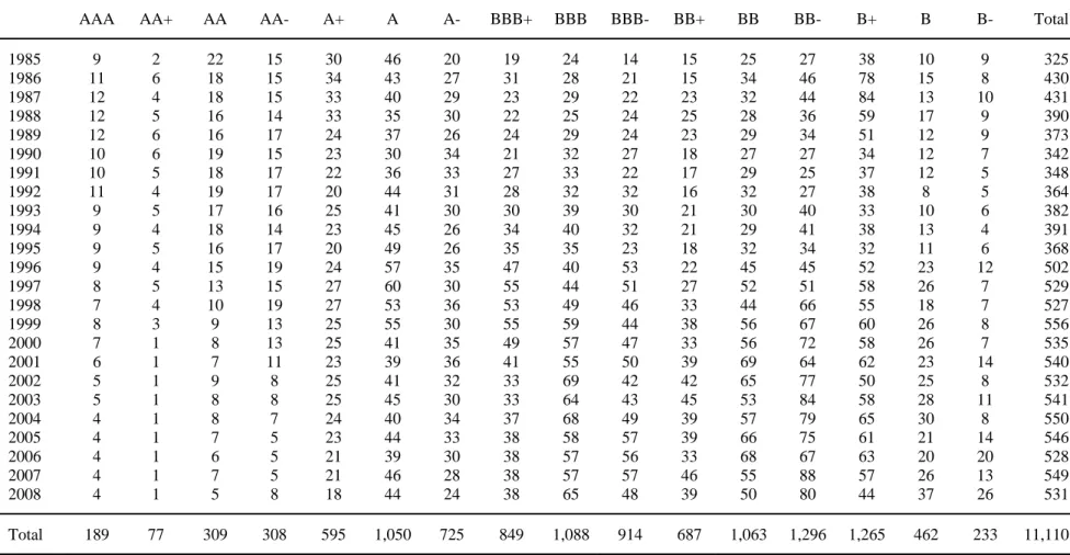
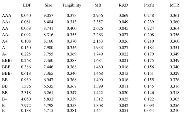
Table 1 presents the distribution of our sample firms by rating and year. Overall, the number of rated firms increases over time during our sample period. In addition, the overall credit quality of our sample firms declines during the sample period.9 Table 2 reports the values of EDF and selected firm characteristics traditionally used in capital structure research for each rating category. The results show that the values of the two different measures of the bankruptcy risk, credit ratings and EDF, are broadly consistent with each other. The results also show discernible patterns in how firm characteristics vary across credit ratings, suggesting that better rated firms tend to be larger and more profitable and tend to have higher market-to-book ratios, R&D, and marginal tax rates.
11 In Table 3, we present the firm characteristics that are important for our subsequent analysis for the subsamples of firms with and without credit ratings. 10 Rated firms tend to be older, larger, more profitable, and tend to have higher asset tangibility, as well as higher book and market debt ratios, marginal tax rates, and market-to-book ratios. About 42.3 (3.0) percent of rated (unrated) firms are in the S&P 500 large-cap index, 15 (4.6) percent are in the S&P400 mid-cap index, and about 76.7 (22.6) percent are traded on the NYSE exchange. Compared to unrated firms, rated firms come from industries with higher fractions of rated firms. Unrated firms tend to have larger R&D and selling expenses and higher operating risk.11 The average one-year default probability is about five percent for unrated firms and 1.6 percent for rated firms. The average rating is about 10, i.e., BBB-.
3. Static tradeoff theory tests 3.1. Empirical design
Our empirical design assumes that firms choose their capital structures as the result of a tradeoff between the tax gains and the financial distress and bankruptcy costs associated with higher levels of debt. Within the context of this simple theory, firms that have the most to gain, in tax benefits, and the least to lose, in financial distress and bankruptcy costs, will choose capital structures that have higher probabilities of bankruptcy. To test this theory we estimate the following regression of the probability of bankruptcy on proxies for the costs and benefits of higher leverage:
. (1)
This approach is similar to the existing tests of the cross-sectional determinants of capital structure that seek to explain debt ratio measures with a set of proxies for tax benefits of
12 financial leverage and costs of financial distress. Our proxies for PrBit are issuer credit ratings and EDF. Following prior studies, our set of firm characteristics, Z, consists of variables such as firm size, asset tangibility, market-to-book, research and development (R&D) expenses, selling expenses, profitability, operating risk, the simulated marginal tax rates (before interest), and firm age. The regressions also include industry indicators to control for fixed industry factors, j, and year indicators to control for macroeconomic effects, t.12
Note that, in contrast to traditional regressions in the literature that examines how rating agencies assign corporate credit ratings (see for example, Pogue and Soldofsky (1969), Pinches and Mingo (1973), and Kaplan and Urwitz (1979), Ederington (1985), Bhojraj and Sengupta (2003), Molina (2005)), the above regressions do not include debt ratio as an explanatory variable. These regressions assume that firms understand that when they choose a specific capital structure, they are, in effect, choosing a specific risk of default, which is measured by credit ratings and EDF.13 In this context, the debt ratio is an endogenous parameter that allows the firm to achieve its chosen probability of bankruptcy.
Since part of our exercise is to re-examine the stylized facts about the empirical evidence for the static tradeoff model, we also run these same regressions with debt scaled by capital (debt + equity), rather than with probability of bankruptcy, as the dependent variable.14
13 As we discussed in the introduction, the focus of this research is on how the coefficients of the regressions with proxies for the probability of bankruptcy as the dependent variable differ from the regressions with the debt ratio dependent variables.
3.2. Self-Selection
It is important to note that not all firms have ratings and that firms that self-select to issue rated debt are likely to be inherently different from firms that do not.15 The comparison of the characteristics of rated and unrated firms in Table 3 confirms this intuition. To the extent that there are unobservable determinants of both the target capital structure and access to the bond market, the coefficients from capital structure models (1) and (2) estimated on the sample of rated firms may be biased.
We address the self-selection problem by explicitly modeling access to the public debt market with a set of instruments that are unrelated to the level of rating and the amount of debt.16 The selection equation has the following form:
. (3)
In equation (3), “Rated” takes the value of one if a firm has a rating and zero otherwise. We use four instruments for modeling the selection decision. Following Faulkender and Petersen (2006), we use proxies that measure the firms’ visibility as our instruments. The idea is that firms that are well known, familiar, and widely followed are likely to face lower costs of introducing public debt issues to the market and hence are more likely to get rated. Our visibility proxies include an indicator variable for firms traded on NYSE and two indicator variables for the presence of the firm in the large-cap and the mid-cap S&P indexes. Firms that belong to these indexes are likely to be more visible than otherwise similar firms.
14 Another way to gauge the accessibility of the public debt markets is to see whether other firms in the same industry have rated debt. If there are comparable firms with outstanding public debt, it may be easier for a firm to participate in the bond market. We, therefore, include a variable measuring the percentage of firms in the same industry that have rated debt as another instrument in our selection model.17
The selection model also includes firm characteristics that proxy for a firm’s propensity to participate in public debt markets. Some firms may have access to the (public) debt market but may choose not to issue long-term bonds. We may, therefore, only observe firms that find long-term debt more valuable due to greater tax shields or contracting benefits and/or lower financial distress costs. For example, large firms and firms with tangible assets are expected to have lower financial distress costs and hence are more likely to have long-term debt. In contrast, firms with high growth opportunities and significant intangible assets may prefer to avoid the debt markets as they face higher costs of financial distress. Our proxies for these factors are R&D intensity, selling expenses, age, and the market-to-book ratio. The effect of profitability on a firm’s propensity to use long-term debt is theoretically ambiguous. While debt may be used less by more profitable firms as a result of their lower external financing needs, such firms may benefit from significant debt tax shields, which should make debt financing more attractive.
Table 4 presents the estimation results for the selection equation (4), estimated as a probit regression using maximum likelihood. The results for selection equations estimated simultaneously with the default probability model (1) and with the book and market leverage specifications of the debt ratio model (2) are similar and are not reported
15 for brevity. The results show that firms that have rated debt are indeed different from the ones that do not have a rating. Consistent with Faulkender and Petersen (2006), the probability of being rated increases with visibility. NYSE traded firms and firms from the S&P500 large-cap and S&P400 mid-cap indexes are more likely to be rated. The probability of being rated increases with the fraction of rated firms in the industry. Firms with higher market-to-book ratios are less likely to be rated. Larger firms and firms with higher asset tangibility are more likely to be rated as they are more likely to have issued long-term debt given their lower information asymmetry and lower costs of financial distress. The probability of being rated increases with R&D and declines with profitability and age. Marginal tax rate, selling expenses and operating risk have an insignificant effect on the likelihood of being rated.
3.3. Capital structure choice results
Table 5 presents the results for the target capital structure models (1) and (2) estimated on the sample of rated firms using a maximum likelihood selection model. The reported z-statistics reflect standard errors adjusted for heteroskedasticity and firm-level clustering. The first and the second sets of results are for the book and the market specifications of the target debt ratio model (2). The third set of results is for the credit rating specification of the probability of bankruptcy model (1). Due to the categorical and ordered nature of credit ratings, the target rating model (1) is estimated using an ordered probit specification that takes into account the fact that the “distances” between the adjacent ratings are not necessarily equal. The fourth set of results is for the probability of bankruptcy model (1) using KMV’s EDF measure of one-year default probability as the dependent variable. The default probability is bounded between zero and one and is a
16 nonlinear function of the underlying determinants of default. To ensure that predicted default rates fall within the range [0,1], we use the following logit transformation of EDF as the dependent variable in the linear regression model (1).18
ln EDFEDF . (4)
Consistent with prior studies, the results in Table 5 show that large firms and firms with high asset tangibility and low R&D expenses tend to choose high debt ratios. The standard interpretation of this result is that large firms with high collateral value of tangible assets and low R&D can choose to be more highly levered because they have low costs of financial distress. However, in the ratings and the EDF models, we find that large size and high asset tangibility are associated with a lower probability of bankruptcy, suggesting that firms with these characteristics choose capital structures that allow them to default less often than small firms and firms with low tangibility. The effect of R&D expenses on the likelihood of bankruptcy is insignificant. These results are inconsistent with the static tradeoff theory that predicts that firms with low bankruptcy costs choose capital structures with a higher risk of default.
The significantly negative coefficient estimates of the marginal tax rate in all four regressions reported in Table 5 imply that both the debt ratios and the likelihood of bankruptcy are lower for firms with higher marginal tax rates. These results are inconsistent with the static tradeoff theory, which predicts that higher marginal tax rates should lead to more leverage and higher default risk.19 One possible explanation for this inconsistency is the correlation between simulated marginal tax rates and past and future operating performance, since firms with bad performance tend to have low marginal tax rates and high leverage ratios. Consistent with this argument, we find in unreported
17 regressions that higher marginal tax rates are associated with increases in leverage, which is consistent with the evidence reported in Graham (1996a) who also examines the effect of the marginal tax rate on changes in leverage.20 However, the coefficient estimates of the marginal tax rate remain significantly negative in all specifications even with additional proxies for past and future performance included.
The effect of operating risk is positive in both the rating and the EDF regressions as well as in the book and the market debt ratio regressions. The positive relation between operating risk and debt ratios or probability of default is inconsistent with intuition that suggests that in the presence of bankruptcy costs, firms with more volatile cash flows, which are exposed to a higher probability of bankruptcy for any given level of debt, should choose less debt. However, there is a theoretical literature that suggests that the relation between financial leverage and operating risk can go either way and the existing evidence is mixed.21
The effect of profitability is consistently negative across the leverage and the default probability regressions, contrary to our expectations under the tradeoff theory. The effect of profitability on leverage is generally interpreted as indicating that asymmetric information (Myers and Majluf (1984)) and personal taxation (Auerbach (1979)) considerations induce firms to retain their profits, which reduces their debt ratios. The above arguments imply that inside equity is a less expensive form of capital than outside equity, which in turn suggests that the costs of achieving a capital structure with less exposure to bankruptcy risk are lower for more profitable firms. The observed negative relation between profitability and probability of default is also consistent with this view.
18 Firms with higher selling expenses tend to choose lower market debt ratios and better ratings. These results are consistent with the hypothesis that firms with more unique products (high selling expenses) target lower probabilities of default because they face high financial distress costs (Titman (1984) and Titman and Wessels (1988)). However, we do not find a reliable relation between EDF or book debt ratio and selling expenses.
The effects of the market-to-book ratio is negative in the debt ratio regressions as well as in the default probability regressions, consistent with the hypothesis that firms with significant growth opportunities (high market-to-book) target capital structures with lower probabilities of default because of either high financial distress costs or to maintain financial flexibility. Hence, market-to-book ratio is the only variable that is consistent with the tradeoff theory in both the Ratings and the EDF regression, but that Selling Expense and the R&D indicator, which are indicators of financial distress costs, are significant in the Ratings regression.
The effect of firm age is negative in all four regressions, though it is insignificant in the book debt ratio regression. This is consistent with the idea that as successful firms grow and mature, they end up with relatively less debt, and hence, lower default probabilities.
3.4. Robustness
The results in the previous section are from regressions estimated on the subsample of rated firms. These firms tend to differ from unrated firms in many respects. While the results reported in Table 5 are based on maximum likelihood models that account for self-selection into the rated group, our conclusions would be strengthened if the results held for all firms, rated as well as unrated.
19 Table 6 presents the least-squares regression results for the EDF specification of model (1) and market and book leverage specifications of model (2) estimated on the sample of all (rated and unrated) firms. The reported t-statistics reflect standard errors adjusted for heteroskedasticity and firm-level clustering. The book and market leverage results in Table 6 are consistent with those reported in Table 5, with the increase in significance in Table 6 being the only difference. The EDF regression results are also, overall, consistent with corresponding results in Table 5. The only difference is that the effects of R&D and selling expenses change from insignificant to significantly negative. These negative estimates are consistent with the predictions of the static tradeoff theory that firms with higher bankruptcy costs should choose capital structures with lower risk of default. However, the results for size, tangibility, and marginal tax rates remain inconsistent with the tradeoff theory, similar to the results in Table 5.
As another robustness test, we reestimated regression model (1) with an alternative measure of bankruptcy risk – the CDS spread. Our CDS spreads sample is much smaller, consisting of observations for about 200 firms over 2006-2008. The results (not reported for brevity) are generally consistent with those reported in Table 5. Specifically, OLS regressions of CDS spreads generate significantly negative coefficient estimates for size and marginal tax rates and insignificant estimates for R&D and tangibility, inconsistent with the predictions of the static tradeoff theory about the effects of these variables on the choice of the exposure to bankruptcy risk. These results should, however, be interpreted with caution, given that the cross section is small, relatively homogeneous, and has inherent selection issues. Indeed, when we estimate the regression in a way that accounts for endogenous selection, the results are no longer significant. It should also be noted,
20 that unlike credit ratings and EDF, CDS spreads incorporate information about recovery rates as well as the likelihood of default.
We also considered the possibility that unobserved firm-specific factors could be driving our earlier results. To see whether the results are consistent with the tradeoff theory when within-firm rather than across-firm variation is considered, we re-estimate both default probability models using linear regressions with fixed firm effects.22 The results are presented in Table 7. In the ratings regression, all three variables (tangibility, size, and marginal tax rate) have signs opposite to the static tradeoff predictions. In the EDF regression only size and marginal tax rate are inconsistent, whereas, consistent with the tradeoff theory, the effect of tangibility is significantly positive.23 Our findings are also robust to alternative specifications of the capital structure regressions (1) and (2) that exclude both firm and industry effects.
Finally, we address the possibility that the discrete nature of ratings and the institutional features of the credit markets may influence our results.24 Kisgen (2009) shows that firms tend to reduce leverage following a ratings downgrade, especially when the rating changes from investment to speculative grade and when commercial paper ratings are affected. This suggests that some firms may have lower leverage than we would expect given their bankruptcy costs (as perhaps measured by tangible assets and size) because of their desire to maintain an investment grade rating. If this were true, we might expect a cluster of firms at BBB- with high values of tangibility and size. Likewise, some firms may have better credit ratings (e.g., A or higher) than their tangible assets or size would suggest, because they want a strong rating to be able to access the commercial paper market.25
21 Our unreported analysis suggests that the targeting of investment grade ratings is not driving our results. Specifically, a univariate analysis of the variation in size and tangibility across ratings categories fails to find that the average values of size and/or tangibility for firms with BBB- or A ratings are significantly higher than the values in neighboring ratings on either side. In addition, our results also continue to hold when we drop BBB-, BBB, A, or A- rated observations from the regressions.
4. Profitability shocks and debt ratio dynamics
As we have just discussed, our finding in the previous section that default probabilities decline with size and tangibility is difficult to reconcile with the static tradeoff theory. One potential explanation for the negative effects of these variables is that they are correlated with the dynamic dimension of risk not picked up by our risk variable. Specifically, smaller firms with fewer tangible assets may have higher transaction and information costs or in other ways find it more difficult to raise equity or sell assets when doing poorly. Such financially constrained firms are likely to have a higher probability of bankruptcy for any given debt ratio.
We investigate this possibility by examining how these firm characteristics affect the ability of firm capital structures to absorb negative shocks to their profitability. If larger firms with more tangible assets are better able to make choices that offset negative shocks, then they may be able to maintain higher debt ratios and still have a lower probability of bankruptcy.
To test whether or not this is indeed the case, we estimate an expanded partial adjustment leverage regression in a switching regression framework represented by the following two equations.
22 it it it Control Variables Shocks [ ] [ ] 1 . (5) it it it it it it Size Tangibility RD MTR Regime 0 1 12 13 13 1 . (6) Equation (5) is a partial adjustment regression of change in debt ratio, DR, on the deviation from the target debt ratio, DR-DR*. Prior research, e.g., Flannery and Rangan (2006), has shown that deviations from target leverage tend to predict future debt ratio changes.26 The standard partial adjustment model is modified as follows. First, we decompose the deviation from the target, DR-DR*, into two components. (DR – DR*)-, which we refer to as leverage deficit, is defined as the difference between the observed and target debt ratios with positive values set to zero. Similarly, (DR – DR*)+, which we refer to as the leverage surplus, is defined as the difference between the observed and target debt ratios with negative values set to zero. By separately considering the debt ratio deficits and surpluses, we account for the possibility that the response by firms to being over-levered and under-levered may not be symmetric. From the point of view of financial risk, our primary focus is on (DR – DR*)+: A firm that can quickly react to offset excess leverage would have a lower probability of bankruptcy.
In addition to deviations from target leverage, regression equation (5) includes profitability and stock market shocks. Here again, to separately measure positive and negative shocks, we use positive and negative changes in profitability (ROA) and positive and negative stock returns, both measured contemporaneously with the change in leverage. From the point of view of financial risk, our primary interest is on negative shocks: A firm with capital structure that is less affected by negative shocks has lower
1 2 1 1 0 ( *)it ( *)it it DR DR DR DR DR
23 probability of bankruptcy. Regression equation (5) also includes past profitability in the form of lagged values of ROA and marginal tax rate as control variables.
Equation (6) represents the switching equation of the endogenous switching model. The independent variables in this equation, firm size and tangibility, endogenously determine the probability that the firm is in one of two regimes. Equations (5) and (6) of the switching regression model are estimated simultaneously using maximum likelihood with robust standard errors adjusted for heteroskedasticity and firm-level clustering.
The results for the switching regression model (5)-(6) are reported in Table 8. The coefficient estimates for the switching equation (6), reported in the first set of results in Table 8, show evidence of existence of two different regimes, which are determined by significant differences in size and tangibility. The second and the third sets of results show coefficient estimates for equation (5) in, respectively, regime 1 and regime 2 and the last column reports the p-values of pairwise tests comparing the coefficient estimates in the two regimes. The results reveal that larger firms and firms with more tangible assets (firms in regime 1) show significantly slower rebalancing toward the target debt ratio, which is inconsistent with our conjecture that firms with these characteristics more quickly adjust their capital structures to offset leverage deficits.
The results also show that, compared to regime 2 firms, capital structures of regime 1 firms are significantly less sensitive to both positive and negative profitability shocks. The sensitivity of regime 1 firms’ capital structures to negative profitability shocks is especially low, it is about twenty times lower than the sensitivity of regime 2 firms and is economically trivial (-0.013). These results imply that firms in regime 1 (large, high tangibility firms) are able to react more quickly to offset the impact of negative
24 profitability shocks on their capital structure.
Consistent with Welch (2004), debt ratio changes are negatively related to stock returns in both regimes. However, the effects for both positive and negative returns are significantly weaker for regime 1 firms. The difference between regime 1 and regime 2 firms is especially large when the impact of negative returns is considered, consistent with larger firms with more tangible assets more successfully neutralizing the effects of negative shocks.
Overall, the significantly weaker effects of negative shocks on capital structure of regime 1 firms imply that firms in regime 1 are able to manage their capital structure dynamics in a manner that reduces their risk of bankruptcy.
5. Conclusions
The static tax gain/bankruptcy cost tradeoff model is clearly a gross simplification of the firm’s capital structure problem. However, since this model provides the central framework of the capital structure theory that we teach our MBA and undergraduate students, and provides the intuitive basis for most of our cross-sectional capital structure tests, it is important to understand the extent to which it explains the data.
The evidence in this paper suggests that the static tradeoff theory fails on a couple of important dimensions. Specifically, we find that firms with the lowest bankruptcy and financial distress costs, i.e., larger firms and firms with more tangible assets, have the lowest probability of bankruptcy. In addition, firms with the lowest marginal tax rates tend to have the highest probability of bankruptcy.
This evidence suggests that the puzzle we identify is related in part to the fact that smaller firms with less tangible assets are more constrained in their ability to take steps,
25 like issuing equity and selling assets, that offset the effect of negative shocks on their capital structures. Specifically, the leverage ratios of these firms increase much more in response to negative shocks than do larger firms with more tangible assets. As a result, these firms may be exposed to more bankruptcy risk even if their current capital structures are more conservative.
While this evidence may explain why firms with relatively high bankruptcy costs tend to have relatively high probabilities of bankruptcy, this is not likely to be a complete explanation for why larger firms with more tangible assets tend to have fairly conservative debt ratios. Our evidence indicates that the ratings of these firms are somewhat less sensitive to their capital structures, since these firms are likely to take steps to offset negative shocks. This in turn indicates that large firms with tangible assets can probably increase their debt ratios, allowing them to take advantage of the tax shields, without suffering substantial increases in their probabilities of bankruptcy.
Finally, it should be noted that our study has implications for the recent literature that compares the magnitude of tax gains and bankruptcy costs. A number of earlier studies (e.g., Andrade and Kaplan (1998), Graham (2000)) argued that U.S. firms appear to be underleveraged, in the sense that expected bankruptcy costs are substantially lower than the value of forgone tax benefits. However, more recent papers, which provide alternative quantitative estimates of expected bankruptcy costs (Almeida and Phillipon (2007)), net benefits of debt (Korteweg (2010)), or the sensitivity of the probability of default to leverage (Molina (2005)), suggest that the firms may not be as underleveraged, on average. Our findings add a cross-sectional dimension to the leverage puzzle. Specifically, we argue that while it may be possible to justify the leverage ratios of either
26 small firms with relatively intangible assets or large firms with relatively tangible assets, that a quantitative model, like Almeida and Phillipon (2007), cannot possibly explain the capital structures of both type firms.
27 References:
Almeida, H., and T. Philippon, 2007, “The risk-adjusted cost of financial distress,”
Journal of Finance 62 2557–2586.
Andrade, G., and S. N. Kaplan, 1998, “How costly is financial (not economic) distress? Evidence from highly levered transactions that became distressed,” Journal of Finance
53, 1443–1493.
Altman, E.I., and H.A. Rijken, 2004, “How rating agencies achieve rating stability,”
Journal of Banking and Finance 28, 2679-2714.
Auerbach, A. J., 1979, “The Optimal Taxation of Heterogeneous Capital,” Quarterly Journal of Economics 93, 589-612.
Baker, M., and J. Wurgler, 2002, "Market Timing and Capital Structure," Journal of Finance 57, 1-32.
Bhojraj, S., and P. Sengupta, 2003, “Effect of Corporate Governance on Bond Ratings and Yields: The Role of Institutional Investors and Outside Directors,” Journal of Business, 76, 455-476.
Black, F., and M. Scholes. 1973. The Pricing of Options and Corporate Liabilities.
Journal of Political Economy 81: 637–54.
Cantillo, M., and J. Wright, 2000, “How do Firms Choose Their Lenders? An Empirical Investigation,” Review of Financial Studies 13, 155-189.
Crosbie, P. J., and J. R. Bohn. 2003. Modeling Default Risk. Moody’s KMV, available at http://www.defaultrisk.com/pp model 35.htm.
Ederington, L. H., 1985, “Classification Models and Bond Ratings,” Financial Review, 20, 237-62.
Faulkender, M., and M. A. Petersen, 2006, “Does the Source of Capital Affect Capital Structure?” Review of Financial Studies 19, 45–79.
Fischer, Edwin O., Robert Heinkel, and Josef Zechner, 1989, Dynamic capital structure choice: Theory and tests, Journal of Finance 44, 19-40
Flannery, M., and K. Rangan, 2006, “Partial Adjustment Toward Target Capital Structure,” Journal of Financial Economics 79, 469-506.
Graham, J.R., 1996a, Debt and the marginal tax rate, Journal of Financial Economics 41, 41-73.
28 Graham, J.R., 1996b, Proxies for the corporate marginal tax rate, Journal of Financial Economics 42, 187-221.
Graham, J.R., 2000, “How big are the tax benefits of debt?” Journal of Finance 55, 1901–1941.
Graham, J.R., M. Lemmon and J. Schallheim, 1998, Debt, Leases, Taxes, and the Endogeneity of Corporate Tax Status Journal of Finance 53, 131-161.
Hennessy, C.A., and T.M. Whited, 2005, “Debt Dynamics,” Journal of Finance, 60, 1129-65.
Hovakimian, A., T. Opler, and S. Titman, 2001, “The Debt-Equity Choice,” Journal of Financial and Quantitative Analysis 36, 1-24.
Kaplan, R. S., and G.l Urwitz, 1979, “Statistical Models of Bond Ratings: A Methodological Inquiry,” Journal of Business 52, 231-262.
Kealhofer, S. 2003a. Quantifying Credit Risk I: Default Prediction. Financial Analysts Journal 59:30–44.
Kealhofer, S. 2003b. Quantifying Credit Risk II: Debt Valuation. Financial Analysts Journal 59:78–92.
Kisgen, D. J., 2006, “Credit Ratings and Capital Structure,” Journal of Finance 61, 1035–1072.
Kisgen, D. J., 2009, “Do Firms Target Credit Ratings or Leverage Levels?” Journal of Financial and Quantitative Analysis, forthcoming.
Korteweg, A., 2010, “The Net Benefits to leverage,” Journal of Finance 65, 2137-2170. Leland, H.E., 1994, “Corporate Debt Value, Bond Covenants, and Optimal Capital Structure,” Journal of Finance, 49, 1213-52.
Lemmon, M. L., M. R. Roberts, and J. F. Zender, 2008, “Back to the Beginning: Persistence and the Cross-Section of Corporate Capital Structure,” Journal of Finance
63, 1575-1608.
Maddala, G.S., 1983, “Limited-Dependent and Qualitative Variables in Econometrics” (Cambridge University Press).
Merton, R. C. 1974. On the Pricing of Corporate Debt: The Risk Structure of Interest Rates. Journal of Finance 29:449–70.
Molina, C. A., 2005, “Are Firms Underleveraged? An Examination of the Effect of Leverage on Default Probabilities,” Journal of Finance 60, 1427-1457.
29 Myers, S. C., 1984, "The Capital Structure Puzzle," Journal of Finance 39, 575-592. Myers, S. C., and N. Majluf, 1984, “Corporate Financing and Investment Decisions When Firms Have Information That Investors Do Not Have,” Journal of Financial Economics 13, 187-221.
Parsons, C., and S. Titman, 2009, “Empirical Capital Structure: A Review,” Foundations and Trends in Finance 3, 1-93.
Pinches, G. E., and K. A. Mingo, 1973, “A Multivariate Analysis of Industrial Bond Ratings,” Journal of Finance 28, 1-19.
Pogue, T. F., and R. M. Soldofsky, 1969, “What's In a Bond Rating?” Journal of Financial and Quantitative Analysis 4, 201-239.
Rajan, R. G., and L. Zingales, 1995, “What Do We Know About Capital Structure? Some Evidence From International Data,” Journal of Finance 50, 1421-1460.
Standard and Poor’s, 2006, “Corporate ratings criteria.”
Strebulaev, I.A., 2007, “Do Tests of Capital Structure Theories Mean What They Say?”
Journal of Finance, 62, 1747-87.
Titman, S., 1984, “The Effects of Capital Structure on a Firm’s Liquidation Decision,”
Journal of Financial Economics, 13, 137-151.
Titman, S., and S. Tsyplakov, 2007, “A Dynamic Model of Optimal Capital Structure,”
Review of Finance, 11, 401-51.
Titman, S., and R. Wessels, 1988, “The Determinants of Capital Structure,” Journal of Finance, 43, 1-19.
Welch, I., 2004, “Capital Structure and Stock Returns,” Journal of Political Economy, 112, 106-31.
Welch, I., 2007, “Common Flaws in Empirical Capital Structure Research,” working paper.
30
Table 1. Distribution of ratings
AAA AA+ AA AA- A+ A A- BBB+ BBB BBB- BB+ BB BB- B+ B B- Total
1985 9 2 22 15 30 46 20 19 24 14 15 25 27 38 10 9 325 1986 11 6 18 15 34 43 27 31 28 21 15 34 46 78 15 8 430 1987 12 4 18 15 33 40 29 23 29 22 23 32 44 84 13 10 431 1988 12 5 16 14 33 35 30 22 25 24 25 28 36 59 17 9 390 1989 12 6 16 17 24 37 26 24 29 24 23 29 34 51 12 9 373 1990 10 6 19 15 23 30 34 21 32 27 18 27 27 34 12 7 342 1991 10 5 18 17 22 36 33 27 33 22 17 29 25 37 12 5 348 1992 11 4 19 17 20 44 31 28 32 32 16 32 27 38 8 5 364 1993 9 5 17 16 25 41 30 30 39 30 21 30 40 33 10 6 382 1994 9 4 18 14 23 45 26 34 40 32 21 29 41 38 13 4 391 1995 9 5 16 17 20 49 26 35 35 23 18 32 34 32 11 6 368 1996 9 4 15 19 24 57 35 47 40 53 22 45 45 52 23 12 502 1997 8 5 13 15 27 60 30 55 44 51 27 52 51 58 26 7 529 1998 7 4 10 19 27 53 36 53 49 46 33 44 66 55 18 7 527 1999 8 3 9 13 25 55 30 55 59 44 38 56 67 60 26 8 556 2000 7 1 8 13 25 41 35 49 57 47 33 56 72 58 26 7 535 2001 6 1 7 11 23 39 36 41 55 50 39 69 64 62 23 14 540 2002 5 1 9 8 25 41 32 33 69 42 42 65 77 50 25 8 532 2003 5 1 8 8 25 45 30 33 64 43 45 53 84 58 28 11 541 2004 4 1 8 7 24 40 34 37 68 49 39 57 79 65 30 8 550 2005 4 1 7 5 23 44 33 38 58 57 39 66 75 61 21 14 546 2006 4 1 6 5 21 39 30 38 57 56 33 68 67 63 20 20 528 2007 4 1 7 5 21 46 28 38 57 57 46 55 88 57 26 13 549 2008 4 1 5 8 18 44 24 38 65 48 39 50 80 44 37 26 531 Total 189 77 309 308 595 1,050 725 849 1,088 914 687 1,063 1,296 1,265 462 233 11,110
31
Table 2. Sample statistics by rating
EDF Size Tangibility MB R&D Profit MTR AAA 0.040 9.057 0.373 2.956 0.069 0.248 0.361 AA+ 0.081 8.404 0.313 2.357 0.049 0.239 0.360 AA 0.058 8.741 0.400 2.626 0.045 0.224 0.364 AA- 0.092 8.316 0.355 2.263 0.027 0.208 0.356 A+ 0.108 8.160 0.370 2.153 0.026 0.210 0.360 A 0.150 7.900 0.356 1.933 0.027 0.184 0.351 A- 0.225 7.755 0.369 1.749 0.022 0.179 0.349 BBB+ 0.268 7.460 0.388 1.684 0.021 0.175 0.349 BBB 0.386 7.446 0.368 1.480 0.016 0.156 0.340 BBB- 0.618 7.365 0.340 1.468 0.013 0.151 0.329 BB+ 0.939 6.947 0.368 1.490 0.016 0.155 0.326 BB 1.376 6.535 0.367 1.399 0.011 0.145 0.316 BB- 2.318 6.261 0.347 1.422 0.020 0.146 0.318 B+ 4.050 5.832 0.339 1.312 0.025 0.122 0.305 B 7.972 5.798 0.353 1.308 0.042 0.093 0.256 B- 10.188 5.715 0.381 1.454 0.051 0.054 0.210 The table presents selected firm characteristics for each rating category. Rating is the S&P issuer-level credit rating. EDF is the Expected Default Frequency from Moody’s KMV. Size is the natural log of sales, adjusted for inflation. Tangibility is the property, plant, and equipment scaled by total assets. Market-to-book is (total assets – Market-to-book equity + market equity)/total assets. R&D is the research and development expense scaled by sales. Profitability is (operating income)/assets. Marginal tax rate is the simulated before-interest marginal tax rate.
32
Table 3
Sample statistics by rated status
Not Rated Rated
S&P500 indicator 0.030 0.423** S&P400 indicator 0.046 0.150** NYSE indicator 0.226 0.767** Probability rated 0.158 0.221** Market-to-book 1.607 1.635* Tangibility 0.284 0.360** R&D 0.037 0.023** R&D indicator 0.663 0.624** Selling expense 0.281 0.201** Profitability 0.123 0.159** Size 4.152 7.091** Operating risk 0.075 0.047**
Marginal tax rate 0.285 0.328**
Age 2.697 3.165** Market debt/capital 0.235 0.317** Book debt/capital 0.291 0.447** EDF (%) 4.974 1.616** Rating 9.823** Observations 35,109 11,110
The table presents the sample means for selected firm characteristics important for our analysis. S&P500 indicator is set to one for firms that belong to S&P500 index. S&P400 indicator is set to one for firms that belong to S&P400 mid-cap index. NYSE indicator is set to one for firms traded on NYSE. Probability rated is the percentage of rated firms in the firm’s industry. Market-to-book is (total assets – book equity + market equity)/total assets. Tangibility is the property, plant, and equipment scaled by total assets. R&D is the research and development expense scaled by sales. R&D indicator is coded one when R&D is not missing. Selling expense is selling, general, and administrative expense over sales. Profitability is (operating income)/assets. Size is the natural log of sales, adjusted for inflation. Operating risk is the standard deviation of profitability measured over the previous four to five years. Marginal tax rate is the simulated before-interest marginal tax rate. Age is the natural log of the Compustat age of the firm. Market debt/capital is (short-term debt + long-term debt)/(short-term debt + long-term debt + market equity). Book debt/capital is (short-term debt + long-term debt)/(short-term debt + long-term debt + book equity). EDF is the Expected Default Frequency from Moody’s KMV. Rating is the S&P issuer-level credit rating. The statistically significant differences between the characteristics of rated and non-rated firms are marked * for 5% level and ** for 1% level.
33
Table 4
Determinants of access to public debt markets
Rated vs. Not rated
Coeff. z-stat. S&P500 indicator 0.512** 6.3 S&P400 indicator 0.151* 2.2 NYSE indicator 0.445** 8.4 Probability rated 1.813** 6.5 Market-to-book -0.099** -4.2 Tangibility 0.788** 6.7 R&D 1.582** 4.7 R&D indicator -0.190** -3.7 Selling expense 0.175 0.9 Profitability -1.212** -6.5 Size 0.649** 28.6 Operating risk 0.551 1.4
Marginal tax rate -0.071 -0.4
Age -0.135** -3.4
Pseudo-R2 0.496
Observations 46,219
The table presents maximum likelihood estimates for the probability of being rated (accessing public debt markets) using a probit specification. S&P500 indicator is set to one for firms that belong to S&P500 index. S&P400 indicator is set to one for firms that belong to S&P400 mid-cap index. NYSE indicator is set to one for firms traded on NYSE. Probability rated is the percentage of rated firms in the firm’s industry. Market-to-book is (total assets – book equity + market equity)/total assets. Tangibility is the property, plant, and equipment scaled by total assets. R&D is the research and development expense scaled by sales. R&D indicator is coded one when R&D is not missing. Selling expense is selling, general, and administrative expense over sales. Profitability is (operating income)/assets. Size is the natural log of sales, adjusted for inflation. Operating risk is the standard deviation of profitability measured over the previous four to five years. Marginal tax rate is the simulated before-interest marginal tax rate. Age is the natural log of the Compustat age of the firm. The dependent and the independent variables are measured contemporaneously. The reported z-statistics reflect robust standard errors adjusted for heteroskedasticity and firm-level clustering. Coefficient estimates significantly different from zero at 5% and 1% level are marked * and **, respectively.
34
Table 5
Static tradeoff model: Rated firms
Book debt/capital Market debt/capital Rating EDF
Coef. z Coef. z Coef. z Coef. z
Market-to-book -0.024** -3.8 -0.097** -15.2 -0.314** -9.1 -0.648** -16.8 Tangibility 0.134** 3.7 0.112** 4.9 -0.390* -2.4 -0.339* -2.2 R&D -0.460** -4.1 -0.244** -3.1 0.864 1.5 -0.890 -1.6 R&D indicator -0.024 -1.8 -0.024* -2.6 -0.175** -2.8 -0.072 -1.3 Selling expense 0.008 0.1 -0.080* -2.1 -1.149** -4.2 -0.363 -1.4 Profitability -0.380** -8.4 -0.493** -14.1 -2.754** -11.5 -3.446** -14.1 Size 0.032* 2.5 0.005 1.0 -0.311** -6.7 -0.129** -3.8 Operating risk 0.356** 3.2 0.272** 3.4 5.192** 10.7 6.686** 12.5
Marginal tax rate -0.245** -5.4 -0.165** -5.3 -1.986** -9.4 -2.861** -12.4
Age -0.012 -1.4 -0.020** -3.0 -0.260** -6.2 -0.286** -6.7
Log-likelihood -10,948 -7,718 -34,888 -29,711
Observations 46,219 46,219 46,219 46,219
Uncensored obs. 11,110 11,110 11,110 11,110
The table presents maximum likelihood estimates of the capital structure regressions with sample selection correction. The sample selection (i.e., the probability of being rated) is modeled using a binomial probit specification from Table 4. The rating regression is modeled using an ordered probit specification. Rating is the S&P issuer-level credit rating. The letter ratings are transformed into numerical equivalents using an ordinal scale ranging from 1 for the highest rated firms (AAA) to 16 for the lowest rated sample firms (B-). EDF is the Expected Default Frequency from Moody’s KMV. Book debt/capital is (short-term debt + long-term debt)/(short-long-term debt + long-long-term debt + book equity). Market debt/capital is (short-long-term debt + long-long-term debt)/(short-long-term debt + long-long-term debt + market equity). Market-to-book is (total assets – book equity + market equity)/total assets. Tangibility is the property, plant, and equipment scaled by total assets. R&D is the research and development expense scaled by sales. R&D indicator is coded one when R&D is not missing. Selling expense is selling, general, and administrative expense over sales. Profitability is (operating income)/assets. Size is the natural log of sales, adjusted for inflation. Operating risk is the standard deviation of profitability measured over the previous four to five years. Marginal tax rate is the simulated before-interest marginal tax rate. Age is the natural log of the Compustat age of the firm. The dependent and the independent variables are measured contemporaneously. Industry and year indicators are included in the models as control variables but are not reported. The reported z-statistics reflect robust standard errors adjusted for heteroskedasticity and firm-level clustering. Coefficient estimates significantly different from zero at 5% and 1% level are marked * and **, respectively.
35
Table 6
Static tradeoff model: Rated and unrated firms
EDF Book debt/capital Market debt/capital
Coef. t Coef. t Coef. t Market-to-book -0.602** -40.7 -0.013** -5.4 -0.066** -34.0 Tangibility -0.315** -3.0 0.215** 12.0 0.170** 11.9 R&D -1.802** -7.6 -0.395** -7.5 -0.225** -6.9 R&D indicator -0.092* -2.3 -0.027** -3.7 -0.025** -4.1 Selling expense -0.753** -6.2 -0.109** -4.8 -0.137** -8.4 Profitability -3.012** -27.1 -0.454** -21.1 -0.393** -26.5 Size -0.302** -25.4 0.025** 13.5 0.011** 7.5 Operating risk 6.061** 24.0 0.237** 4.8 -0.020 -0.6 Marginal tax rate -3.091** -26.1 -0.279** -12.3 -0.159** -9.5
Age -0.286** -9.8 -0.015** -2.8 -0.022** -5.4
R2 0.585 0.178 0.324
Observations 46,219 46,219 46,219
The table presents estimates of the capital structure regressions on a full sample of rated and unrated firms. EDF is the Expected Default Frequency from Moody’s KMV. Book debt/capital is (short-term debt + term debt)/(short-term debt + term debt + book equity). Market debt/capital is (short-term debt + long-term debt)/(short-long-term debt + long-long-term debt + market equity). Market-to-book is (total assets – book equity + market equity)/total assets. Tangibility is the property, plant, and equipment scaled by total assets. R&D is the research and development expense scaled by sales. R&D indicator is coded one when R&D is not missing. Selling expense is selling, general, and administrative expense over sales. Profitability is (operating income)/assets. Size is the natural log of sales, adjusted for inflation. Risk is the standard deviation of profitability measured over the previous four to five years. Marginal tax rate is the simulated before-interest marginal tax rate. Age is the natural log of the Compustat age of the firm. The dependent and the independent variables are measured contemporaneously. Industry and year indicators are included in the models as control variables but are not reported. The reported t-statistics reflect robust standard errors adjusted for heteroskedasticity and firm-level clustering. Coefficient estimates significantly different from zero at 5% and 1% level are marked * and **, respectively.
36
Table 7
Static tradeoff model: Within-firm determinants of default probability
Rating EDF Coef. t Coef. t Market-to-book -0.193** -4.3 -0.517** -36.6 Tangibility -1.250** -2.9 0.703** 5.4 R&D -1.981* -2.2 -0.826** -3.1 R&D indicator 0.564* 2.5 0.061 1.1 Selling expense -2.190** -3.4 -0.644** -4.6 Profitability -2.527** -7.5 -2.513** -25.9 Size -1.046** -10.6 -0.188** -7.9 Operating risk 3.742** 4.9 3.381** 15.4
Marginal tax rate -1.136** -3.9 -1.659** -19.8
Age -0.813** -3.2 -0.070 -1.1
R2 0.526 0.506
Observations 11,110 46,219
The table presents the estimates of the bankruptcy probability regressions with fixed firm and year effects. Rating is the S&P issuer-level credit rating. The letter ratings are transformed into numerical equivalents using an ordinal scale ranging from 1 for the highest rated firms (AAA) to 16 for the lowest rated sample firms (B-). EDF is the Expected Default Frequency from Moody’s KMV. Market-to-book is (total assets – book equity + market equity)/total assets. Tangibility is the property, plant, and equipment scaled by total assets. R&D is the research and development expense scaled by sales. R&D indicator is coded one when R&D is not missing. Selling expense is selling, general, and administrative expense over sales. Profitability is (operating income)/assets. Size is the natural log of sales, adjusted for inflation. Risk is the standard deviation of profitability measured over the previous four to five years. Marginal tax rate is the simulated before-interest marginal tax rate. Age is the natural log of the Compustat age of the firm. The dependent and the independent variables are measured contemporaneously. The reported t-statistics reflect robust standard errors adjusted for heteroskedasticity and firm-level clustering. Coefficient estimates significantly different from zero at 5% and 1% level are marked * and **, respectively.
37
Table 8
Debt ratio dynamics in a switching regression framework
Switching: Regime 2 vs. Regime 1 Change in debt/capital: Regime 1 Change in debt/capital: Regime 2 Regime 2 vs. 1
Coeff. z-stat. Coeff. z-stat. Coeff. z-stat. p-value
(Actual – Target) (-) -0.045** -12.2 -0.270** -21.9 0.000 (Actual – Target) (+) -0.018 -1.6 -0.120** -12.3 0.000 Profitability shock (+) -0.053** -4.0 -0.117** -4.9 0.029 Profitability shock (-) -0.013* -2.5 -0.258** -11.4 0.000 Return (+) -0.006** -4.1 -0.024** -9.0 0.000 Return (-) -0.018** -7.3 -0.111** -16.6 0.000 Profitability -0.001 -0.2 -0.067** -6.0 0.000
Marginal tax rate 0.004 1.0 0.095** 8.4 0.000
Intercept 0.283** 7.8 -0.040** -19.4 -0.142** -16.5 0.000
Size -0.035** -8.6
Tangibility -0.095* -2.3
Log-likelihood 38,430
Observations 35,875
The table presents maximum likelihood estimates of an endogenous switching regression, where the likelihood function endogenously sorts the observations in one of the two regimes of debt ratio dynamics. The dependent variable in the structural equation with two regimes is the change in the book debt/capital. Book debt/capital is (short-term debt + long-term debt)/(short-term debt + long-term debt + book equity). (Actual – Target)(-) is the difference between the lagged and the target debt/capital ratios, with positive values reset to zero. (Actual – Target)(+) is the difference between the lagged and the target debt/capital ratios, with negative values reset to zero. Target debt/capital is the predicted value from the book debt/capital regression from Table 6. Profitability is (operating income)/assets. Profitability shock (+) is the change in profitability, with the negative values reset to zero. Profitability shock (-) is the change in profitability, with the positive values reset to zero. Return (+) is the one-year stock return, with the negative values reset to zero. Return (-) is the one-year stock return, with the positive values reset to zero. Marginal tax rate is the simulated before-interest marginal tax rate. Size is the natural log of sales, adjusted for inflation. Tangibility is the property, plant, and equipment scaled by total assets. The dependent variable, change in debt/capital, is measured contemporaneously with profitability shocks and stock returns. All other independent variables are lagged. The reported z-statistics reflect robust standard errors adjusted for heteroskedasticity and firm-level clustering. Coefficient estimates significantly different from zero at 5% and 1% level are marked * and **, respectively
38
1
There are number of potential reasons for why our results and Graham et al. (1998) findings on marginal tax rates in debt ratio regressions might be inconsistent. For example, our variable constructions are slightly different. For example, we use both book leverage and market leverage and scale them by total market capitalization, (we scale book debt either by book debt plus market equity or by book debt plus book equity), whereas Graham scales book debt by market value of assets (total assets minus book equity plus market equity). However, the negative relation between the debt ratios and the marginal tax rate appears to be quite robust with respect to various leverage definitions, subsamples, and the inclusion/exclusion of various variables in the regression specification. We can, however, replicate the positive coefficient (but not its magnitude) found in Graham et al. (1998) with their specific specification. However, this result appears to be sensitive to the inclusion and exclusion of various control variables.
2
See Standard and Poor’s Corporate Ratings Criteria (2006), page 9, for the discussion on the definition of issuer credit ratings. 3
Moody’s uses Vasicek-Kealhofer structural model (Kealhofer (2003a), Kealhofer (2003b)) which extends the contingent claim framework of Black and Scholes (1973) and Merton (1974). Crosbie and Bohn (2003) provide further detail on how Moody’s implements the Vasicek-Kealhofer model to construct their EDF measure. The measure we use is constructed from the recently recalibrated model (2007) which incorporates a larger default dataset and improved estimation techniques that derive the EDF term structure from credit migration. The previous calibration of the model was developed with data available in 1995.
39 4
The Compustat data item for credit rating is SPLTICRM, which is defined as the Standard & Poor’s current opinion of an issuer’s overall creditworthiness, apart from its ability to repay individual obligations, and it focuses on the obligor’s capacity and willingness to meet its long-term financial commitments.
5
Observations with credit ratings indicating default are excluded from our analysis. We also exclude observations with CCC-, CCC, and CCC+ ratings as the number of firms with such ratings is very small in our sample.
6
See Graham (1996a, 1996b) and Graham et al. (1998) for details of the procedure used to simulate the marginal tax rates. 7
Compustat coverage of credit ratings starts in 1985. 8
The exception is the book debt ratio, which is trimmed to exclude observations with book debt ratios of one or higher. 9
In a recent report, Standard & Poor’s Credit Rating Services documents that industrial firms display a steady decline in average credit quality over the past decade from a median rating of A in 1980, to BBB- in 1997, to BB- in 2007.
10
Age is the natural log of the number of years since the firm appeared first in Compustat. Size is the natural log of sales (SALE), adjusted for inflation. Tangibility is the property, plant, and equipment (PPENT) scaled by total assets (AT). Profitability is operating income (OIBDP) scaled by lagged total assets. Market-to-book ratio is market value of assets over total assets. Market value of assets is (total assets – book equity + market equity). Book equity is the book value of stockholders’ equity, plus balance sheet deferred taxes and investment tax credit if available (TXDITC), minus the book value of preferred stock. Depending on availability, we use the