A meta-learning system for multi-instance
classification
Gitte Vanwinckelen and Hendrik Blockeel
Department of Computer Science, KU Leuven, Belgium
Abstract. Meta-learning refers to the use of machine learning
meth-ods to analyze the behavior of machine learning methmeth-ods on different types of datasets. Until now, meta-learning has mostly focused on the standard classification setting. In this ongoing work, we apply it to multi-instance classification, an alternative classification setting in which bags of instances, rather than individual instances, are labeled. We define a number of data set properties that are specific to the multi-instance set-ting, and extend the concept of landmarkers to the multi-instance setting. Experimental results show that multi-instance classifiers are very sensi-tive to the context in which they are used, and that the meta-learning approach can indeed yield useful insights in this respect.
1
Introduction
Machine learning is largely an empirical science. When a researcher develops a new learning algorithm, they typically evaluate it by comparing its perfor-mance with that of existing algorithms on a collection of datasets. From these experiments, we try to understand which types of problems are suitable for a certain algorithm, and which are not. A more systematic approach to under-stand the inductive bias of different learners is to derive meta-characteristics from each dataset, and learn a model that can predict which learner best suits which dataset. This is the purpose of meta-learning. Several such studies have been conducted in the past. For an overview, we refer to Vilalta and Drissi (2002) and Giraud-Carrier (2008).
One subfield of machine-learning is multi-instance learning. It emerged from a specific type of learning problem were there is incomplete information about the labels of the instances. Therefore, instances are grouped together in a bag, which then receives a label, instead of each instance receiving a label separately. Multi-instance learning was originally proposed by Dietterich et al (1997) in the context of drug activity prediction. Here, the goal was to predict whether a molecule smelled musky or not, based on its type and shape. Some types of molecules never smelled musky, regardless of their shape; other types of molecules smelled musky when they took on one or more specific shapes. What made this problem different from a standard supervised learning problem, was that when smelling a molecule, only its type could be observed, not its shape. Consequently, molecules of the same type but different shape were grouped together in a bag, which then received a label indicating the presence of a musky smell.
Later, multi-instance learning was also applied in, for instance, content-based information retrieval (Andrews et al, 2003; Maron and Ratan, 1998; Li et al, 2009; Fu et al, 2011; Zhou et al, 2005), music retrieval (Mandel and Ellis, 2008), protein family modeling (Tao et al, 2004), and medical diagnosis (Fung et al, 2007).
The term multi-instance learning has been used with slightly different mean-ings over time. Here, we use it in the sense of what is sometimes called “general-ized multi-instance learning”. Instances are organ“general-ized into bags that are labeled positive or negative; the number of instances in a bag is not fixed. The task is to learn a function that predicts the label of a bag. Due to the variable size of bags, a bag cannot be represented as a single vector without loss of information; multi-instance learners somehow have to handle this complication.
Several types of multi-instance learners have been proposed in the past, and they vary quite strongly in terms of the assumptions they make. This begs the question whether one can predict, using a meta-learning approach, which methods are suitable for which datasets. In this paper, we present ongoing work in this direction. The contributions are as follows.
First, we propose a number of dataset descriptors that are specific to the multi-instance setting, and evaluate their relevance experimentally.
Second, we propose and evaluate two landmarking approaches for multi-instance classification. The term landmarking was first introduced by Pfahringer et al (2000) for regular (“single-instance”) learning. It refers to running a num-ber of computationally cheap classifier systems on a dataset, and recording the behavior of these systems, in the hope that this will provide information re-garding what methods (including much more expensive ones) are suitable for this dataset. As multi-instance methods tend to be computationally more ex-pensive by nature, we use single-instance learners for landmarking; this implies that the multi-instance datasets somehow have to be turned into (necessarily non-equivalent) single-instance datasets. We investigate two different methods for doing so.
The remainder of the paper is structured as follows. In Section 2, we in-troduce terminology on multi-instance learning. In Section 3, we present our meta-learning approach. In Section 4, we describe our meta-dataset, including the multi-instance learners and the datasets on which it is based. In Section 5, we report experimental results, and in Section 6 we conclude.
2
Definition and terminology
2.1 Multi-instance learning
Let X be the instance space andB={pos, neg} the binary set of class labels. Standard binary classification, which we here call thesingle-instancesetting, can be defined as follows. We are given a datasetDconsisting of elements (xi, f(xi)) with xi ∈ X an instance and f(xi) ∈ B its label according to an unknown functionf :X →B. The learning task is to find the functionf.
The original definition ofmulti-instance learning, as proposed by Dietterich et al (1997), is as follows. We are given a dataset that consists of bags Bi of instances where each bag has a label; the number of instances in a bag is vari-able. Each instance is described by a single vector xij ∈ X. We are given bag labels, and we assume that a bag is labeled positive if it contains at least one positive instance, and negative otherwise. This is what we call thestandard MI
assumption. From this information, we are to either learn a function that can
classify bags or instances.
Over time, the definition of multi-instance learning has become more broad. Namely, any kind of relationship may exist between the properties of the in-stances in a bag and its bag label, and we are to learn a function that can classify bags. This is referred to as the generalized multi-instance learning set-ting. Many definitions of the relationship between instances and bag label can exist. In fact, the standard MI assumption can be considered as an example. An overview is provided by Foulds and Frank (2010). It is this generalized MI setting that we consider in this paper.
2.2 Meta-learning
The meta-learning task we consider is defined as follows. We are given
infor-mation about a collection of multi-instance classification tasks, consisting of the evaluation of different multi-instance learners l1, l2, ... on a set of datasets
D1, D2, .... For each of these tasks we also have an estimate of the performance of
the resulting classifierl(D) in terms of the Area Under the ROC Curve (AUC). From this information we want to predict which learner to apply when presented with a new dataset. We therefore construct a meta-datasetM by extracting var-ious properties from the original multi-instance learning tasks. Each instance in M consists of the extracted properties of one multi-instance task D, and is labeled with the multi-instance learnerl that achieved the best performance on
D. This results in a new standard supervised learning problem.
3
Our approach
One approach of constructing a meta-dataset is to extract statistical and infor-mation theoretic properties from the original datasets. Examples of such proper-ties include number of features, number of classes, ratio of examples to features, correlation between features and target concept, number of nominal attributes (Giraud-Carrier, 2008). In the specific case of multi-instance learning, another property that can be extracted is the number of instances in a bag. Since each bag in the dataset can have a different number of instances in it, this informa-tion may have to be summarized by for instance computing the mean number of instances in bag from the given dataset.
Another approach which was first introduced by Pfahringer et al (2000) and is reported to have stronger predictive power than statistical properties, is land-marking. A landmarker is a fast and cheap learner that indirectly gives us infor-mation about the properties of a dataset by means of its performance. Because
multi-instance datasets are typically imbalanced, we chose Area Under the ROC Curve (AUC) as a performance measure.
Applying multi-instance algorithms can be computationally expensive, there-fore we first derive new single-instance datasets from the original multi-instance datasets, on which we will then apply a set of landmarkers. Whether these new classification tasks are equivalent to the original ones depends on the properties of the original multi-instance data and learner assumptions. We derive the new datasets in two different ways:
1. We label each instance with the label of its bag. Many instances will have a positive label in the dataset even if they are really negative. The opposite will not occur, so we get a dataset with one-sided class noise. This approach corresponds with the standard multi-instance assumption (Section 2). 2. We map the instances in a bag to a single feature vector by averaging each
feature over these instances. We now learn a classifier based on aggregate in-formation about a bag, instead of on the individual instances. This approach corresponds with a type of collective assumption where every instance con-tributes equally to the bag label.
As landmarkers we chose four learners with reasonably different biases:
– A decision stump based on the attribute that maximizes the gain-ratio
– Naive Bayes
– Nearest neighbors with one neighbor
– Logistic regression
4
The meta-learning dataset
The meta-learning dataset is based on the evaluation of fourteen multi-instance learners on datasets from three different domains in terms of AUC. These evalua-tions have been performed in the context of other ongoing work on multi-instance learning (Vanwinckelen et al, submitted 2014). The description of the datasets and multi-instance learners is also adopted from this text. Reusing experiments allows for easy investigation of the behavior of learning algorithms under dif-ferent conditions, an idea that has been put forward before by Vanschoren and Blockeel (2008) with the introduction of an experiment database.
4.1 Multi-instance datasets
Real-world: SIVAL.The SIVAL repository1 (Settles et al, 2008) is from the
area of content-based image retrieval (CBIR). It contains 1500 images where each image contains one out of 25 different complex objects. The images are parti-tioned into 31 or 32 segments, i.e., the instances. An instance in this dataset consists of 30 features expressing color and texture information about the image
1
segment and its four closest neighbors. The repository contains 25 multi-instance datasets where in turn each of the 25 objects is considered positive, while the other 24 objects are considered negative. In positive bags, the percentage of pos-itive instances varies from 3.1% to 90.6%, with an average of 25.5%. Each of the 25 training sets consists of 20 positive and 20 negative bags, and the remaining 1460 bags are used as test set. These training sets are quite small because they were originally proposed in the context of active learning. We decided to leave the datasets in their original form because this facilitates replicability of the ex-periments. However, increasing training set size could lead to better performance of the meta-learner as it makes the landmarker scores more reliable.
Semi-synthetic: Text categorization. We use 20 MI text categorization
datasets extracted by Settles et al (2008) from the 20 newsgroups corpus2. Each dataset contains 100 bags and is balanced on the bag level. The size of the bags (number of instances) varies from 8 to 84, with an average of 40. A bag is a collection of short texts from the newsgroups. In positive bags, the percentage of positive instances varies from 2% to 7%, with an average of 3.6%. This is a high-dimensional dataset; each instance is characterized by 200 TFIDF features. The bags were artificially created by in turn considering one newsgroup as pos-itive, while taking the other newsgroups as negative and i.i.d. sampling texts from the newsgroups such that around 3% of the texts in a bag are from the positive category.
Semi-synthetic UCI datasets.We have constructed some more semi-synthetic
MI datasets from five source datasets taken from the UCI repository (Merz and Murphy, 1996): Adult (Kohavi, 1996), Pima Indians Diabetes (Smith et al, 1988), Spam (Cranor and LaMacchia, 1998), Tic-Tac-Toe (Aha, 1990) and Blood Trans-fusion Service Center (Yeh et al, 2009). We selected these datasets because they are imbalanced, which is useful for constructing MI datasets, since MI datasets that are balanced on the bag-level contain more negative than positive instances. All datasets are binary classification problems; we kept the labels unchanged, except for Tic-Tac-Toe, where we inverted the instance labels in order to have a majority of negatives.
We have constructed multiple MI datasets by choosing instances i.i.d. and grouping them into bags, controlling for bag size and positive/negative ratio in positive bags. We say that a MI dataset is in bag-configuration ‘X/Y’ if each bag in the dataset contains Y instances, of which in each positive bag there are exactly X instances positive. For each source dataset, we use MI datasets in configurations 1/2, 1/3 and 2/3; for the two largest (Adult and Spam) we additionally use 1/4, 2/4, 1/5, 2/5, 1/10 and 2/10. All MI datasets are balanced on the bag level: 50% of the bags is positive and 50% is negative. To construct a MI dataset in a particular bag-configuration, we randomly sampled the required number of positive instances and negative instances from the respective source dataset. The number of bags in each MI dataset is the highest possible number for which we can sample without replacement before exhausting the source dataset, except for Adult, where for computational reasons we retained only 1200 bags
2
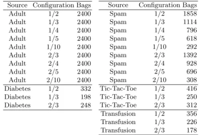
for each label, randomly chosen. Table 1 gives an overview of the resulting 27 MI datasets. In comparison to the SIVAL and text datasets, the UCI datasets have large training set sizes, few features and relatively small bag sizes.
Table 1. Characteristics of the semi-synthetic MI datasets: source dataset, bag
con-figuration and number of bags in the MI dataset. Source Configuration Bags
Adult 1/2 2400 Adult 1/3 2400 Adult 1/4 2400 Adult 1/5 2400 Adult 1/10 2400 Adult 2/3 2400 Adult 2/4 2400 Adult 2/5 2400 Adult 2/10 2400 Diabetes 1/2 332 Diabetes 1/3 198 Diabetes 2/3 248
Source Configuration Bags
Spam 1/2 1858 Spam 1/3 1114 Spam 1/4 796 Spam 1/5 618 Spam 1/10 292 Spam 2/3 1392 Spam 2/4 928 Spam 2/5 696 Spam 2/10 308 Tic-Tac-Toe 1/2 416 Tic-Tac-Toe 1/3 250 Tic-Tac-Toe 2/3 312 Transfusion 1/2 356 Transfusion 1/3 226 Transfusion 2/3 178 4.2 Multi-instance algorithms
We performed experiments with fourteen MI algorithms available in the Weka data mining tool (Witten and Frank, 2005): MIDD (Diverse Density) (Maron and Lozano-P´erez, 1998), MIEMDD (Expectation-Maximization Diverse Den-sity), MDD (Modified Diverse Density with collective assumption) (Zhang and Goldman, 2001), MISVM, which is a Weka implementation of the maximum pattern margin formulation mi-SVM by (Andrews et al, 2003), MIOptimalBall (Auer and Ortner, 2004), MILR (Logistic Regression) (Ray and Craven, 2005), logistic regression with the arithmetic mean model, referred to as MILRC from now on (Dong, 2006), MIRI (Bjerring and Frank, 2011), AdaBoost.M1 (Fre-und and Schapire, 1995) with a Multi Instance Tree Inducer (MITI) as a base classifier (Blockeel et al, 2005)(Dong, 2006), Citation-kNN (Wang and Zucker, 2000), TLD (Two-Level Distribution) (Xu, 2003), SimpleMI with the J48 classi-fier (Dong, 2006), MIWrapper with the J48 classiclassi-fier (Frank and Xu, 2003), and MISMO, which is a Weka implementation of the normalized set kernel (NSK) by (G¨artner et al, 2002).
The parameter settings are as follows. MISMO uses the radial basis function (RBF) kernel withγ equal to 0.01 and the regularization parameter C equal to 1.0. MISVM uses the linear kernel with the regularization parameter C being
1.0. We also ran the experiments with the RBF kernel but found that this kernel did not lead to good performance on the text and SIVAL datasets. For MILR, the ridge coefficient equals 10−6. For Citation-kNN the number of citers and
references both equal 5.
4.3 Multi-instance learner performance
We measure the AUC of each MI learning algorithm on each MI dataset. For the SIVAL datasets we perform 20 independent runs for each image class and average these results. For each run 20 randomly drawn positive bags and 20 randomly drawn negative bags were selected for training. For the text datasets and the UCI datasets we use 10-fold cross-validation.
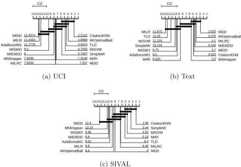
Figure 1 presents the global rankings of the fourteen learners taken over all datasets from each category (SIVAL, text and UCI datasets) with a critical difference (CD) diagram as described by Demsar (2006). This CD diagram is ob-tained by computing a ranking of the algorithms for each dataset and afterwards computing average ranks. A Friedman test is used to test if the performance dif-ference between the algorithms is statistically significant at p = 0.05. If this is the case, we proceed with a post hoc Nemenyi test to find pairwise signif-icant performance differences between the algorithms. The mean rank of each algorithm over all datasets of a given category is indicated on the horizontal axis. The highest rank corresponds to the best performance. Algorithms that are connected do not have significantly different performance.
The CD diagrams make it clear that the AUC varies over a wide range. The overall rankings depend on the characteristics of the datasets and is different for each domain of datasets. The top three algorithms for the UCI datasets are MIDD, MILR, and AdaBoost.M1 with MITI as base learner. The classifier that is ranked highest most often is AdaBoost.M1-MITI, for 44.4% of the datasets. For the newsgroup datasets MILR is ranked highest most often, on 50% of the datasets. TLD is also among the best performing algorithms, which it was not for the UCI datasets. This algorithm models the class conditional probability distributions of the features. An approach that is appropriate for the text data where the features actually represent word frequencies, an approximation of word probability. We can see that the distance based approaches such as the different versions of Diverse Density (MDD, MIEMDD and MIDD), MIOptimalBall, and CitationKNN do not perform well on the text datasets. This is explained by the high dimensionality of the datasets (200 features). Finally, on the SIVAL datasets MIDD has the highest AUC most often, on 44.0% of the datasets.
5
Experiments
5.1 Experimental setup
In total we evaluated fourteen learners, which results in a multi-class meta-learning problem. However, treating the problem as such did not result in any
CD 1413121110 9 8 7 6 5 4 3 2 1 2.2222CitationKNN 3.8889MIOptimalBall 4.4074TLD 4.7593MISVM 5.7407SimpleMI 7.3148MIRI 7.537MDD 7.5556 MILRC 7.6296 MIWrapper 8 MIEMDD 9.5 MISMO 11.7778 AdaBoostM1 12.2593 MILR 12.4074 MIDD (a) UCI CD 1413121110 9 8 7 6 5 4 3 2 1 2.825MDD 4.075MIOptimalBall 4.1MILRC 4.425MIEMDD 4.7MIDD 4.825CitationKNN 5.5MIWrapper 8.625 MIRI 9.5 AdaBoostM1 9.75 MISMO 10.125 SimpleMI 11.325 MISVM 12.35 TLD 12.875 MILR (b) Text CD 1413121110 9 8 7 6 5 4 3 2 1 1.96CitationKNN 3.44SimpleMI 4.52MISVM 5.16MIRI 6.4TLD 6.48MILRC 8MDD 8.4 MIOptimalBall 8.8 MILR 9.52 AdaBoostM1 9.8 MIEMDD 9.88 MISMO 10.24 MIWrapper 12.4 MIDD (c) SIVAL
Fig. 1.Critical difference diagrams for the global ranking of all learning algorithms in
terms of AUC aggregated over all UCI, text, or SIVAL datasets
useful model. The meta-properties that can distinguish between the multi-instance learners are different for each algorithm. We therefore convert the problem into a set of binary classification problems by predicting for each possible combination of two learners which one has the highest AUC. With fourteen learners, there are 91 pairs of classifiers. As a meta-learner we chose an unpruned CART decision tree learner with a maximum depth of two to avoid overfitting3. We evaluated
the meta-model in terms of accuracy.
Because we have three categories of datasets of which the properties are very different, we performed experiments for each category of datasets and evaluated the meta-model with leave-one-out cross-validation.
5.2 Results: UCI datasets
In Section 3 we discussed a number of statistical and information-theoretic meta-properties that can be extracted from the multi-instance datasets. However, because we have datasets from three different domains, where in each domain most of these properties are very similar, we initially only use the number of features an instance has, and the noise level of the dataset, measured by the percentage of positive instances in a positive bag. Figure 2 shows the results for the evaluation of the decision tree model learned from the UCI meta-dataset. The figure compares the predictive accuracy of the meta-model with that of a
3
MIDDMILRAdaB.MISMOMIEMDDWrapperMILRCMDDMIRISimpleMISVMTLDOptBallCitation MIDDMILR AdaB. MISMO MIEMDD WrapperMILRC MDDMIRI SimpleMISVM TLD OptBall Citation
Fig. 2.Comparison of a majority class predictor with a decision tree meta-model for
the UCI datasets. Meta-properties are the number of features of an instance and noise level of the dataset. Blue circles represent classifier pairs for which the meta-model has highest accuracy, red circles for which the majority class predictor does. The area of the circle is proportional to the difference in accuracy between the two models.
classifier that always predicts the majority class (which corresponds to always using the multi-instance learner that is best on average). Blue circles represent classifier pairs for which the meta-model has highest accuracy, red circles for which the majority class predictor does. The area of the circle is proportional to the difference in accuracy between the two models.
The high accuracy of the meta-model on many classifier pairs in comparison to that of the majority classifier shows that the number of features and the noise level are useful properties for determining the most performance multi-instance learner. Investigating the decision trees, we see that the number of features is most often the determining factor in predicting the winning classifier. Each of the five source datasets (Adult, Diabetes, Spam, Tic-tac-toe, and Transfusion) from which the multi-instance datasets were constructed has a different number of features. This means that the meta-model is mostly learning to distinguish between these five dataset types.
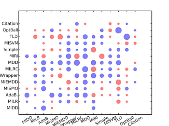
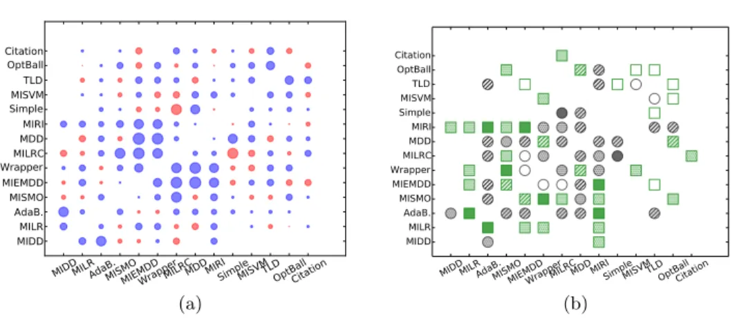
In a next experiment, we predict the learner with the highest AUC based exclusively on the eight landmarking properties defined in Section 3. Figure 3a shows the results for this experiment. We observe that the landmarking approach has worse performance than the previous approach. Although there are a few cases where the landmarking model performs best. Examples are (MILR,MIDD), (MIRI,MIEMDD), (MIRI,MILRC), and (TLD,CitationKNN).
Figure 3b shows the importance of the different landmarkers by, for each pair of classifiers, showing the landmarker that was selected as the root node of the decision tree meta-model when trained on the complete meta-dataset, i.e., the landmarker with the highest information gain ratio. The symbols are defined as follows. Green landmarkers are computed on the averaged single-instance datasets, and gray landmarkers on the one-sided noisy single-instance datasets.
MIDDMILRAdaB.MISMOMIEMDDWrapperMILRCMDDMIRISimpleMISVMTLDOptBallCitation MIDDMILR AdaB. MISMO MIEMDD WrapperMILRC MDDMIRI SimpleMISVM TLD OptBall Citation (a)
MIDDMILRAdaB.MISMOMIEMDDWrapperMILRCMDDMIRISimpleMISVMTLDOptBallCitation MIDDMILR AdaB. MISMO MIEMDD WrapperMILRC MDDMIRI SimpleMISVM TLD OptBall Citation (b)
Fig. 3.(a) Comparison of a majority class predictor with a decision tree meta-model
based on landmarking for the UCI datasets. (b) Landmarkers with highest gain-ratio for classifier pairs where the meta-model performs best.
The decision stump, naive Bayes, nearest neighbors, and logistic regression clas-sifier are respectively identified by a empty, colored, hatched (//), and dotted symbols (.). We only show the landmarkers where the meta-model outperformed the majority class predictor. From this figure, we see that the landmarker with the highest gain ratio often changes from one classification pair to the other.
5.3 Results: Text datasets
Exclusively based on number of features and the training set size, we cannot make predictions for the text and SIVAL datasets because these properties are the same for each dataset from these domains. We therefore employ landmarkers again. As can be seen from Figure 4a, our meta-model does not perform very well on the text datasets. In most cases it is better to predict the multi-instance algorithm that performs best on the majority of text datasets. Figure 4b again shows the landmarkers having the highest gain-ratio for the cases where the meta-model wins.
5.4 Results: SIVAL datasets
For the SIVAL datasets our meta-model based on landmarking again did not outperform the majority class predictor in many cases, as can be seen from Figure 5a. Regarding the most important landmarkers, Figure 5b shows that for the SIVAL datasets this is frequently naive Bayes, trained on one sided noisy data. This is in contrast with the UCI datasets, where this landmarker was selected only once for (SimpleMI,MILRC).
As an alternative, we therefore investigated if the distribution of positive in-stances in a bag has any predictive power. Our meta-properties in this case are
MILRTLDMISVMSimpleMISMOAdaB.MIRIMDDOptBallMILRCMIEMDDMIDDCitationWrapper MILRTLD MISVM Simple MISMOAdaB. MIRI MDD OptBallMILRC MIEMDDMIDD Citation Wrapper (a) MILRTLDMISVMSimpleMISMOAdaB.MIRIMDDOptBallMILRCMIEMDDMIDDCitationWrapper MILRTLD MISVM Simple MISMOAdaB. MIRI MDD OptBallMILRC MIEMDDMIDD Citation Wrapper (b)
Fig. 4.(a) Comparison of a majority class predictor with a decision tree meta-model
based on landmarking for the text datasets. (b) Landmarkers with highest gain-ratio for classifier pairs where the meta-model performs best.
the average percentage of positive instances in a bag, and the variance of the percentage of positive instances over all bags in a given dataset. Note that this information is not necessarily available in a generalized multi-instance setting, as there is no assumption about the existence of instance labels. Nevertheless, this is an interesting property to investigate. Figure 6 shows the results of this experiment. As can be seen, the distribution of positive instances in a bag in-fluences the performance of the multi-instance learners. Inspecting the learned decision trees, we see for example that for MDD, MILRC, TLD, and MIWrapper, the decision tree learns that AdaBoost.M1-MITI outperforms these classifiers on datasets with a large average percentage of positive instances, i.e., a low noise level. It is known that for regular supervised learning, AdaBoost is prone to overfitting on noisy datasets. This also appears to be the case for multi-instance learning.
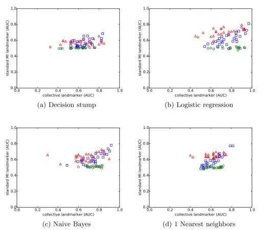
5.5 Meta-feature analysis
In this section we do an exploratory analysis of the performance of the different landmarkers, in order to better understand the relevance of those landmarkers as meta-features, and the influence of the domains of the multi-instance datasets on them. For this purpose, we constructed the four scatter plots shown in Fig-ure 7. Each plot shows the AUC of the standard MI landmarker versus that of the collective landmarker, for one single-instance algorithm. Each point on a plot corresponds to the AUC on one multi-instance dataset. If we look at the scatter plots, we can make some interesting observations. First, we see that, in all cases except the decision stump, we observe three clusters of results, based exclusively on the AUC’s of the standard MI assumption landmarkers, which cor-respond with the three multi-instance dataset domains. However, for the SIVAL
MIDDWrapperMISMOMIEMDDAdaB.MILROptBallCitationSimpleMISVMMIRI TLDMIRCMDD MIDD WrapperMISMO MIEMDDAdaB. MILR OptBall CitationSimple MISVMMIRI TLD MIRC MDD
MIDDWrapperMISMOMIEMDDAdaB.MILROptBallCitationSimpleMISVMMIRITLDMIRCMDD MIDD WrapperMISMO MIEMDDAdaB. MILR OptBall CitationSimple MISVMMIRI TLD MIRCMDD
Fig. 5.(a) Comparison of a majority class predictor with a decision tree meta-model
based on landmarking for the SIVAL datasets. (b) Landmarkers with highest gain-ratio for classifier pairs where the meta-model performs best.
and the newsgroup datasets, the landmarker AUC’s are otherwise very similar within one cluster. Oppositely, when looking at the AUC’s of the the collective MI assumption landmarkers, several multi-instance datasets can be found that are from a different domain, but still have similar AUC’s. However, within one domain the AUC’s of these landmarkers are more spread out. Finally, for the UCI datasets, we also notice a positive linear correlation between the collective and the standard MI landmarker AUC’s.
6
Conclusions
In recent years, several algorithms have been proposed specifically for multi-instance learning. In this work, we evaluated whether we can predict which of these algorithms is most suitable for a given multi-instance dataset. We tackled this problem by extending the landmarking approach introduced by Pfahringer et al (2000) to the multi-instance setting. We found that which landmarkers have best predictive performance depends on the domain of the datasets, and the multi-instance learners that are compared. The most suitable algorithm for a given dataset strongly depends on the domain of that dataset. A meta-model that was learned on one domain does not necessarily transfer to a different domain. These observations have consequences for empirical research on multi-instance learning. They illustrate that it is insufficient to evaluate multi-instance learners on different datasets from a certain problem domain, instead, evaluation should be done on datasets from several different domains. If not, the domain selection introduces a bias.
MIDDWrapperMISMOMIEMDDAdaB.MILROptBallCitationSimpleMISVMMIRI TLDMIRCMDD MIDD WrapperMISMO MIEMDDAdaB. MILR OptBall CitationSimple MISVMMIRI TLD MIRC MDD
Fig. 6.Comparison of a majority class predictor with a meta-model based on the mean
and variance of the percentage of positive instances in a bag.
0.0 0.2 0.4 0.6 0.8 1.0 collective landmarker (AUC)
0.0 0.2 0.4 0.6 0.8 1.0
standard MI landmarker (AUC)
(a) Decision stump
0.0 0.2 0.4 0.6 0.8 1.0 collective landmarker (AUC)
0.0 0.2 0.4 0.6 0.8 1.0
standard MI landmarker (AUC)
(b) Logistic regression
0.0 0.2 0.4 0.6 0.8 1.0 collective landmarker (AUC)
0.0 0.2 0.4 0.6 0.8 1.0
standard MI landmarker (AUC)
(c) Naive Bayes
0.0 0.2 0.4 0.6 0.8 1.0 collective landmarker (AUC)
0.0 0.2 0.4 0.6 0.8 1.0
standard MI landmarker (AUC)
(d) 1 Nearest neighbors
Fig. 7.Each scatter plot shows the AUC of two meta-features that are constructed by
the same landmarking algorithm, but based on a different MI assumption. UCI datasets (blue triangle), newsgroup datasets (Green circle), SIVAL datasets (Red square).
Bibliography
Aha D (1990) Incremental constructive induction: An instance-based approach. In: Proc. of the 7th International Conference on Machine Learning, Morgan Kaufmann, pp 117–121
Andrews S, Tsochantaridis I, Hofmann T (2003) Support vector machines for multiple-instance learning. In: Advances in Neural Information Processing Sys-tems 15
Auer P, Ortner R (2004) A boosting approach to multiple instance learning. In: Proc. of the 15th European Conference on Machine Learning, Lecture Notes in Computer Science, vol 3201, Springer, pp 63–74
Bjerring L, Frank E (2011) Beyond trees: Adopting miti to learn rules and en-semble classifiers for multi-instance data. In: Proc. of the 24th Australian Joint Conference on Artificial Intelligence, Springer, pp 41–50
Blockeel H, Page D, Srinivasan A (2005) Multi-instance tree learning. In: Proc. of the 22d International Conference on Machine learning, ACM Press, pp 57–64 Cranor L, LaMacchia B (1998) Spam! Communications of the ACM 41(8):74–83 Demsar J (2006) Statistical comparisons of classifiers over multiple data sets.
Journal of Machine Learning Research 7:1–30
Dietterich T, Lathrop R, Lozano-P´erez T (1997) Solving the multiple instance problem with axis-parallel rectangles. Artificial Intelligence 89(1-2):31–71 Dong L (2006) A comparison of multi-instance learning algorithms
Foulds J, Frank E (2010) A Review of Multi-Instance Learning Assumptions. Knowledge Engineering Review 25:1–25
Frank E, Xu X (2003) Applying propositional learning algorithms to multi-instance data. Tech. rep., University of Waikato
Freund Y, Schapire R (1995) A decision-theoretic generalization of on-line learn-ing and an application to boostlearn-ing. In: Proc. of the 2d European Conference on Computational Learning Theory, Springer-Verlag, pp 23–37
Fu Z, Robles-Kelly A, Zhou J (2011) MILIS: multiple instance learning with instance selection. IEEE Transactions on Pattern Analysis and Machine In-telligence 33(5):958–977
Fung G, Dundar M, Krishnapuram B, Rao R (2007) Multiple instance learning for computer aided diagnosis. In: Advances in Neural Information Processing Systems 19
G¨artner T, Flach P, Kowalczyk A, Smola A (2002) Multi-instance kernels. In: Proc. of the 19th International Conference on Machine Learning, Morgan Kaufmann, pp 179–186
Giraud-Carrier C (2008) Meta-learning–a tutorial
Kohavi R (1996) Scaling up the accuracy of naive-Bayes classifiers: A decision-tree hybrid. In: Proc. of the 2d International Conference on Knowledge Dis-covery and Data Mining, AAAI Press, vol 7, pp 202–207
Li Y, Kwok J, Tsang I, Zhou Z (2009) A convex method for locating regions of interest with multi-instance learning. In: Proc. of the European Conference on Machine Learning and Knowledge Discovery in Databases, Springer-Verlag
Mandel M, Ellis D (2008) Multiple-instance learning for music information re-trieval. In: Proc. of the 9th International Conference on Music Information Retrieval, pp 577–582
Maron O, Lozano-P´erez T (1998) A framework for multiple-instance learning. In: Advances in Neural Information Processing Systems 11
Maron O, Ratan A (1998) Multiple-instance learning for natural scene classifi-cation. In: Proc. of the 15th International Conference on Machine Learning, Morgan Kaufmann, pp 341–349
Merz C, Murphy P (1996) UCI repository of machine learning databases. Http://archive.ics.uci.edu/ml/
Pfahringer B, Bensusan H, Giraud-Carrier C (2000) Meta-learning by landmark-ing various learnlandmark-ing algorithms. In: ICML, pp 743–750
Ray S, Craven M (2005) Supervised versus multiple instance learning: An em-pirical comparison. In: Proc. of the 22d International Conference on Machine Learning, ACM Press, vol 22, pp 697–704
Settles B, Craven M, Ray S (2008) Multiple-instance active learning. In: Ad-vances in Neural Information Processing Systems 20
Smith J, Everhart J, Dickson W, Knowler W, Johannes R (1988) Using the ADAP learning algorithm to forecast the onset of diabetes mellitus. In: Proc. of the Symposium on Computer Applications and Medical Care, pp 261–265 Tao Q, Scott S, Vinodchandran N, Osugi T (2004) SVM-based generalized
multiple-instance learning via approximate box counting. In: Proc. of the 21th International Conference on Machine learning, Morgan Kaufmann
Vanschoren J, Blockeel H (2008) Investigating classifier learning behavior with experiment databases. In: Preisach C, Burkhardt H, Schmidt-Thieme L, Decker R (eds) Data Analysis, Machine Learning and Applications, An-nual Conference of the Gesellschaft f¨ur Klassifikation e.V., Albert-Ludwigs-Universit¨at Freiburg, March 7-9, 2007, Springer, pp 421–428
Vanwinckelen G, Tragante Do O V, Fierens D, Blockeel H (submitted 2014) Instance-level accuracy versus bag-level accuracy in multi-instance learning Vilalta R, Drissi Y (2002) A perspective view and survey of meta-learning.
Ar-tificial Intelligence Review 18(2):77–95
Wang J, Zucker J (2000) Solving the multiple-instance problem: A lazy learning approach. In: Proc. of the 17th International Conference on Machine Learning, Morgan Kaufmann, pp 1119–1126
Witten I, Frank E (2005) Data Mining: Practical machine learning tools and techniques
Xu X (2003) Statistical learning in multiple instance problems. Master’s thesis Yeh I, Yang K, Ting T (2009) Knowledge discovery on RFM model using
Bernoulli sequence. Expert Systems With Applications 36(3P2):5866–5871 Zhang Q, Goldman S (2001) EM-DD: An improved multiple-instance learning
technique. In: Advances in Neural Information Processing Systems 14 Zhou Z, Xue X, Jiang Y (2005) Locating regions of interest in cbir with
multi-instance learning techniques. In: Proc. of the 18th Australian Joint conference on Advances in Artificial Intelligence, Springer-Verlag, pp 92–101