Validation of default probability models: A stress testing approach

(1)

Validation of default probability models: A stress testing approach

☆

Fábio Yasuhiro Tsukahara

a

, Herbert Kimura

b

, Vinicius Amorim Sobreiro

b,

⁎

, Juan Carlos Arismendi Zambrano

c,d a

Midway Finance, 500 Leão XIII, São Paulo, São Paulo, 02526-000, Brazil b

University of Brasília, Department of Management, Campus Darcy Ribeiro, Brasília, Federal District, 70910-900, Brazil c

Department of Economics, Federal University of Bahia, Rua Barão de Jeremoabo, 668-1154, Salvador, Brazil d

ICMA Centre, Henley Business School, University of Reading, Whiteknights, Reading RG6 6BA, United Kingdom

a b s t r a c t

a r t i c l e i n f o

Article history: Received 15 July 2015

Received in revised form 31 May 2016 Accepted 28 June 2016

Available online 8 July 2016

This study aims to evaluate the techniques used for the validation of default probability (DP) models. By generating simulated stress data, we build ideal conditions to assess the adequacy of the metrics in different stress scenarios. In addition, we empirically analyze the evaluation metrics using the information on 30,686 delisted US public companies as a proxy of default. Using simulated data, weﬁnd that entropy based metrics such as measureMare more sensitive to changes in the characteristics of distributions of credit scores. The em-pirical sub-samples stress test data show thatAUROCis the metric most sensitive to changes in market conditions, being followed by measureM. Our results can help risk managers to make rapid decisions regarding the valida-tion of risk models in different scenarios.

In summary, the Basel II Accord allows banks to develop internal models for measuring risk (BCBS, 2006; Kiefer, 2009) and the Basel III Accord aims to enhance the stability of theﬁnancial system by strengthening risk coverage and highlighting the importance of on-and off-balance sheet risks, including derivatives exposure (BCBS, 2011). In addition, the Accords also require validation of risk models to determine,1_{qualitatively and quantitatively, the models'} perfor-mance and adherence to the institution's goals. In this context,

Stein (2007)states that the validation process is of great importance, since it allows the beneﬁts generated by the use of risk models to be fully obtained. However, effectively validating risk models is still a great challenge, because this is a recent aspect of banking regulation and the primary methods are still under development. In particular, credit model validation has major impediments, i.e., the small

number of observations to accurately evaluate model performance (Lopez & Saidenberg, 2000).2

Many validation techniques of models for bank risk management have been proposed or submitted in recent years, for market risk (Alexander & Sheedy, 2008; Boucher, Daníelsson, Kouontchou, & Maillet, 2014), credit risk (Lopez & Saidenberg, 2000; Agarwal & Tafﬂer, 2008), and model risk (Kerkhof & Melenberg, 2004; Alexander & Leontsinis, 2011; Alexander & Sarabia, 2012; Colletaz, Hurlin, & Pérignon, 2013).Blöchlinger (2012)presents a methodology where the validation of default probability (DP) is produced over credit rating methodologies.Medema, Koning, and Lensink (2009)proposes a prac-tical methodology for validation of statisprac-tical models ofDPfor portfolio of individual loans where no credit rating can be associated. However, there are no studies that attempt to identify or guide managers regard-ing which model is most appropriate for a given situation. With regard to the methods for estimating credit risk parameters,DPmodels are, ac-cording toBCBS (2005a), those that have the most developed validation

☆ This document is a collaborative effort.

⁎ Corresponding author.

E-mail addresses:[email protected](F.Y. Tsukahara),[email protected] (H. Kimura),[email protected](V.A. Sobreiro),[email protected] (J.C.A. Zambrano).

1 _For_{ﬁnancial institutions to be able to use their internal models to calculate capital} re-quirements, the Basel II Accord requires that the models be validated by an independent in-ternal team. For this inin-ternal validation process it is necessary to develop techniques to consistently assess the performance of the models used. In this study, we present some val-idation techniques that are widely used in theﬁnancial market for assessment of models, such asKSandAR, and other less traditional measures, such asCIERand measureM.

2

The growth of credit activity is an important aspect of economic development, be-cause credit is a major source of funds for private and public organizations (Hagedoorn, 1996). However, increases in credit supply bring more exposure to credit risk and, in ex-treme cases, overreliance on credit can compromise the stability of thefinancial system (Abou-El-Sood, 2015; Arnold, Borio, Ellis, & Moshirian, 2012). Economic crises, such as the one in 2008, indicate a need for greater control and regulation offinancial institutions by supervisors and for the development of risk management models. In this context, the Basel I, II, and III Accords are examples of how regulatory agencies are concerned with se-curing a solid internationalfinancial system; they are dynamically adjusting their require-ments due to an ever-changing economic environment.

Contents lists available atScienceDirect

(2)

methodology.Tasche (2006)separates the performance validation pro-cess for these models into two parts, discriminative ability and calibration.

Our contribution to the literature is twofold. First we evaluate the stress test the adequacy of the primary models for risk management and thereby support the decision-making of managers regarding the model selection process. More speciﬁcally, we present the characteris-tics and main properties of different techniques that allow a manager to choose among classic validation models, such as the Kolmogorov–

Smirnov (KS) statistic, Accuracy Ratio (AR), and Brier Score, and newer validation models, such as the Conditional Information Entropy Ratio (CIER) and MeasureM. The stress test simulation3is carried out in two phases: (i) an assessment of the performance of models to separate good and bad borrowers among the risk groups is performed, (ii) the ac-curacy of the probabilities estimated by each model is evaluated.4_The models were applied to credit portfolios, which were compiled using Monte Carlo simulations, to identify good and bad borrowers and how the characteristics (e.g., dependencies or moments) of these portfolios impacted the results of the models. According toZott (2003), when there are significant limitations on gathering empirical data and vari-ables have complex interrelationships, simulation may be useful and can actually lead to superior insights into the phenomenon.5The objec-tive of this study is not to exhausobjec-tively explore the subject but rather to enable managers to quickly identify a small number of optimal models. Second, we analyze the default probability validation metrics using controlled sub-samples of market data. Our empirical stress analysis in-cludesfinancial data of from 30,686 public USfirms from 1950 and 2014, using delisting information as a proxy for default. We develop a methodology that aggregates different groups of years by high–low mean, variance, and correlation related to thefinancial explanatory variables. Although using empirical data does not allow as total control as using simulated data, the method gives some control over the distribution of credit scores and dependence among variables. Therefore, we can also analyze the behavior ofDPevaluation metrics on empirical sub-sample data.

In the case of controlled stress simulations, for independent explan-atory variables, we found that (i) the measureMwas the only metric able to detect changes in the mean of the explanatory variables,6 while there was no metric sensitive to changes in the variances; (ii) all metrics were very sensitive to the number of observations; there-fore, the study can help in the validation of models for the retail and large corporations segment. In the case of controlled stress simulations, for dependent explanatory variables, we found that (i) the only metric that captured a performance decrease for both increases and decreases in the correlation parameter was measure M, all other measures exhibited an increase in performance as the strength of the correlation was decreased; (ii) modeling using theTcopula and Gaussian copula provided no difference in the sensitivity results of the metrics.

The remainder of this study is structured as follows: inSection 2, a literature review of credit is presented;Section 3 and 4address the aspects used to compare the models and their results;Section 5

presents a empirical application; inSection 6, the primary conclusions are presented and discussed.

2. Literature review

The Basel II Accord aims to improve the awareness of the_financial institutions regarding their credit risk (Hakenes & Schnabel, 2011). The Basell II Accordfirst pillar aims to guide the calculation of minimum capital requirements, i.e., it reviews the main ideas presented in the Basel I Accord. The minimum capital requirement is calculated based on the Internal Rating Based (IRB) method, which is generally estimated internally by a bank based on the following parameters: (i)DP; (ii) Ex-posure at Default (EAD); (iii) Loss Given Default (LGD); and (iv) Maturi-ty (M). It is worth noting that in the simplified version of theIRB, it is only necessary to calculate theDPvalue because the other parameters are defined by regulatory bodies. From this point of view, the calculation ofDPbecomes crucial.

2.1. Validation tests for default probability models

Two of the most used validation tests are the Cumulative Accuracy Pro_ﬁle (CAP) curve andARdeveloped bySobehart, Keenan, and Stein (2000a). Their calculation is performed by ranking all parties based on the scores estimated by the model. Once ranked, for a certain cutoff score, it is possible to identify the fraction of defaults and non-defaults with scores that are less than the cutoff score. TheCAPcurve is obtained by calculating these fractions for all possible cutoff points, as shown inFig. 1.

According toEngelmann, Hayden, and Tasche (2003), theARcan be deﬁned by:

AR¼aR

aP; ð

1Þ

whereaR,aPare the areas deﬁned inFig. 1. The closer theARis to one, the

greater the discriminative ability of the model.

The Receiver Operating Characteristic (ROC) curve and the area under the ROC curve are other widely used validation measures developed byTasche (2006). TheROCcurve is obtained by plotting HR(C) versusFAR(C), whereHR(C) is the hit rate andFAR(C) the false alarm rate at scoreC. According toEngelmann et al. (2003), the higher the area under theROCcurve of the model, the better the performance. Considering the ideal situation, i.e., anROCarea equal to 1, the area may be calculated using Eq.(2):

AUROC¼Z1 0

HR FARð Þd FARð Þ: ð2Þ

The Pietra Index developed byPietra (1915)7_{is a widely used index,} whose geometric interpretation corresponds to half of the shortest distance between theROCcurve and the diagonal. This index can be calculated as: PI¼ ffiffiffi 2 p 4 maxcjHR Cð Þ−FAR Cð Þj ð3Þ

Sobehart et al. (2000a)deﬁned theCIERmeasure according to: CIER¼H0ð ÞP −H1

H0ð ÞP ; ð

4Þ

whereH0(P),H1are entropy functions developed byJaynes (1957)and related to Kullback-Leibler (KL) distance, with the purpose ofﬁnding a function with conditions of continuity, monotonicity, and composition law, that represents the uncertainty of a probability distribution.

Keenan and Sobehart (1999)deﬁned the measureH0(p) as the entropy of a binary event for whichpis the default rate of the sample.

3

Simulated portfolios to study credit risk have been explored in the literature. For in-stance,Kalkbrener, Lotter, and Overbeck (2004)develops an importance sampling Monte Carlo technique to study capital allocation for credit portfolios andJobst and Zenios (2005) use simulation to analyze the sensitiveness of credit portfolio values to default probability, recovery rates, and migration of ratings. In addition,Hlawatsch and Ostrowski (2011) study loss given default based on simulated datasets to analyze the synthesized loan portfolios.

4_{Since there are many classiﬁcation techniques used for credit scoring (}

Baesens et al., 2003), performance measurement is necessary to assess model adequacy (Verbraken et al., 2014).

5_{Davis, Eisenhardt, and Bingham (2007)}_{presents a reference to the theory developed} using simulation methods.

6

Explanatory variables are any variables that can lead to a causal explanation of the re-lationships in default, such as the ones included in theZ-scoreofAltman (1968). 7

(3)

TheBRIERscore was originally proposed byBrier (1950); this metric has the objective of measuring the accuracy of forecasts provided by a given model; and it was initially proposed to measure the accuracy of weather forecasts. The Brier Score can be calculated according to:

BRIER¼_N1X N i¼1 Pi−Oi ð Þ2 ; ð5Þ

wherePicorresponds to the probability of occurrence of the event given

by the model for thei−thcomponent of the sample; andOi

corre-sponds to a binary variable (1/0), where one means that the event was observed and zero means that the event was not observed. A per-fectDPmodel would estimate a probability equal to one for observed default events and zero probability for default events that are not observed. Consequently, the Brier Score would be equal to zero, i.e., a Brier Score closer to zero indicates higher accuracy of the model.

MeasureMis proposed byOstrowski and Reichling (2011), and it aims to evaluate the discriminative ability of the default models. Let (aD,i,aND,i) be areas of default and non-default, and (rD,iandrND,i) hit

rates of default and non-default for thei−thrating , (Ostrowski & Reichling, 2011) deﬁned a measure of the performance of the model:

m¼X k i¼1 HRi rD;i−aD;i þFARi rND;i−aND;i ð6Þ

wherekcorresponds to the total number of ratings. Note that this measure is not yet standardized, which precludes direct comparison of two different models. To standardise this measure, the values ofmmax andmminare calculated and the standardizedMmeasure is:

mmin¼ Xk i¼1

minHRiRD;i−aD;i;FARirND;i−aND;i; ð7Þ

The value ofmshould be in the range of 0 and 1, where 1 indicates perfect predictive ability of the model.

According to the studies of Kolmogorov–Smirnov,Lilliefors (1967)

presents a procedure to test if a set ofnobservations is derived from a normal distribution. In a simpliﬁed manner,Lilliefors (1967)proposes a hypothesis test for measureD which is the absolute difference between the accumulated distribution function of the sample; and the

normal accumulated distribution function with mean and variance equal to those of the sample. To validate credit risk models, it is worth noting that the aim is not to analyze the normality of a distribution but rather to check whether the model can distinguish defaults and non-defaults. For such a purpose, theKS statistic can be used, as described inJoseph (2005), to quantify the greatest distance between the accumulated distribution of defaults and non-defaults.KScan be calculated using:

KS¼maxjFDð Þ−S FNDð Þj;S ð8Þ

whereFDcorresponds to the accumulated distribution function of

default cases,

FNDcorresponds to the accumulated distribution function of

non-default cases, andScorresponds to the score.

The parameter of information value (IV) proposed byTasche (2006)

measures how default and non-default events are distributed different-ly among ratings. LetRibe thei−thrating,pD(Ri) the ratio of defaults of

thei₋thrating, andpND(Ri) the ratio of non-defaults of thei−thrating.

Then, the value ofIVcan be calculated following (Joseph, 2005) using: IV¼X i pDð ÞRi −pNDð ÞRi ½ In pDð ÞRi pNDð ÞRi ; ð9Þ

It is important to highlight that highIVvalues indicate high discrim-inative ability (Tasche, 2006).

2.2. Studies of the validation of DP models

Although the process of validation of credit risk models required by Basel II is still relatively new to the globalﬁnancial market, some studies about model performance measurement techniques had been previous-ly published. Among these studies, the following are noteworthy.

Keenan and Sobehart (1999)presented the following techniques to measure the performance of predictive default modelsCAP,AR,CIER, and Mutual Information Entropy (MIE). Using a dataset that included data from 9,000 public companies, covering the years of 1989 through 1999, and containing 530 default events, the authors applied a return based model and four additional prediction models (Altman, 1968; Shumway, 2001; Merton, 1974; Sobehart et al., 2000a), the authors were able to conclude that the tests were effective and measured

(4)

distinct aspects of the model.Keenan and Sobehart (1999)emphasized that theCAPcurve and theARmeasure the discriminative ability of the default model prediction and theCIERandMIEassess whether different models interact by adding information or are simply redundant;Hanley and McNeil (1982)andEngelmann et al. (2003)presented the Receiver Operator Characteristic (ROC) technique and explained its use in the context of validation of rating models. There exists a relationship be-tween bebe-tween theARand the area under theROCcurve (AUROC) that can be calculated by:

AR¼2AUROC−1; ð10Þ

Karakoulas (2004)presented a validation methodology for credit scoring andDPmodels for the retail segment and small companies. The author also argued that theKSstatistic has the limitation of not referring to where the point of maximum distance occurs and that the AUROC is more generic regarding this point and therefore better;

Joseph (2005)presented a validation methodology based on several tests, and theﬁnal evaluation of the model was based on the average performance of the models in these tests. In addition to theAR,ROC, KS, and Kullback Leibler measures, Joseph (2005) used other measures, such as the mean difference andIV.

Ostrowski and Reichling (2011)found that theARandAUROC measures can, in certain circumstances, lead to erroneous conclu-sions and cause low-performance models to be rated well according to these indicators. This observation is in accordance with

Engelmann et al. (2003), as the author states that if the distribution of default events is bimodal, a perfect model can have anAUROC equal to that of a random model. Furthermore, Ostrowski and Reichling (2011)proposed another measure calledM, to measure the performance of the model and applied this new measure in the credit rating models used by the agencies Standard & Poor's and Moody's. Considering the period from 1982 to 2001, the authors observed that the AUROCmeasure behaved in a stable manner compared with measureM, which exhibited high variability in the measurement of model performance.

3. Numerical stress test simulation

Taking into account that different simulated situations lead to distinct behaviors of the metrics it is possible to analyze how the characteristics of the default phenomenon could inﬂuence a broad set of evaluation metrics. Consequently, we studied the traditional performance measures likeKS,AUROCandAR(BCBS, 2005b; Hand, 2009; Keenan & Sobehart, 1999; Marshall, Tang, & Milne, 2010; Ostrowski & Reichling, 2011; Verbraken, Bravo, Weber, & Baesens, 2014) as well as other less common metrics like Pietra,BRIER, CIER,Kullback-Leibler(KL),Information Value(IV) and measureM (Joseph, 2005; BCBS, 2005b; Ostrowski & Reichling, 2011; Izzi, Oricchio, & Vitale, 2012).

Our analysis of the validation techniques can be divided into two parts:

1. In theﬁrst part, good and bad borrower distributions were simulated according to an arbitrary scoring rule and assigned to variableYB. The

properties of the distributions were then changed. With this setting, it was possible to analyze the impact of these changes on the values calculated using the validation techniques. This part of the methodology can be summarized by

(a). Generation of the variableYBof good and bad borrowers using a

Monte Carlo simulation approach with a normal distribution to tag subjects into good and bad borrowers;

(b). Generation of explanatory variablesX1,X2by a normal distri-bution with different mean and volatility, depending on whether the subject was tagged as a good or bad borrower in step 1;

(c). Generation of default variableYby a gamma distribution; (d). Association of Xi,i = 1,2 with Y using a bi-stochastic

matrix; and,

(e). Calculation of the performance of the entropy-based valida-tion measures by their sensitivity to changes inX1andX2. 2. In the second part of the study logistic models were developed

from simulated portfolios that contained a default event and other independent variables. As a consequence, it was possible to analyze how changes in the variables, or in the existing relationships be-tween them, affected the values measured by the techniques studied. This part of the methodology includes

(a). Use of the logistic model to calculate the probabilityPof the default of a subject depending onX1andX2;

(b). Generation of credit scores usingP, having n-ratings (10 in our numerical simulation) for the classiﬁcation of the subject; (c). Calculation of the number of realized defaults from the variableY

obtained in theﬁrst part of the methodology; and.

(d). Calculation of the performance of rating-based validation measures by their sensitivity to changes inX1andX2.

The methodology presented associated changes in the distribution properties ofX1,X2, depending on whether is it is a good or bad borrow-er, with the performance of the techniques for the validation ofDP. We then analyzed how different changes in distribution parameters and re-lationships between variables affect the performance of the validation techniques.8

3.1. Normal distribution simulation for good and bad borrowers

Applying the Monte Carlo simulation technique, different portfolios that contained normal distributions of good and bad borrowers were generated. All portfolios consisted of 30,000 simulations and a bad borrower rate of approximately 10%. The parameters changed in the different portfolios were the mean scores of good and bad borrowers and the deviations of both distributions. Although the deviations were changed, this change was performed on both distributions such that in all portfolios, the deviation of the bad borrower distribution was equal to the deviation of the good borrower distribution. The procedure used to construct the portfolio was as follows:

1. Random classiﬁcation of the portfolio subjects into good and bad borrowers;

2. Determination of the mean score of the distribution of good borrowers, mean score of the distribution of bad borrowers. and standard deviations of both distributions; and,

3. Assignment of a score to each subject using the Monte Carlo simulation technique

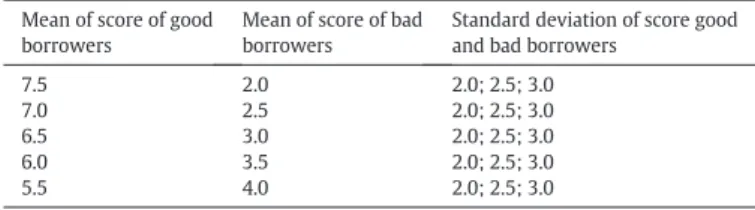
Table 1presents the parameters used in the different simulated portfolios.

We generated simulated data for the relevant variables to analyze the effects of parameters of the credit score distributions of good and bad borrowers on the validation metrics. Once the sim-ulations were completed, theKS,AUROC,AR, andPietra Index techniques were applied. Subsequently, each portfolio had its score ranked, and the 30,000 components were distributed into 10 ratings of 3,000 components each. Rating 1 contained the lowest scores, and rating 10 contained the highest scores. Through separation in ratings, it was possible to estimate the values of theCIER,Kullback LeiblerandIVvalidation techniques.

8

The use of simulated data makes it possible to have control over the various relation-ships among variables. Therefore, we can analyze the adequacy of the validation tech-niques in a controlled environment. When using empirical data from real default situations, the very complexity of the phenomenon can preclude an analysis focused solely on the variables of interest, jeopardizing the study of the validation of models. Neverthe-less, we also conducted an empirical analysis aiming to identify the behavior of validation models under real world credit events. Therefore, our study also allows the comparison of results using both simulated and real-world data.

(5)

3.2. Normal distribution simulation for good borrowers and bimodal distribution simulation for bad borrowers

Similar to portfolios with normal score distributions for good and bad borrowers, portfolios that contained a bimodal distribution for bad borrowers were developed using Monte Carlo simulations, with 30,000 observations per portfolio and a bad borrower rate of 10%. The difference compared with using a normal distribution for bad borrowers is that rather than a normal distribution, the bimodal distribution consists of two normal distributions, one with a mean score that is less than the distribution mean of good borrowers (DM1) and another with a higher mean score (DM2). For these portfolios, the distribution deviations of good borrowers,DM1andDM2, were kept constant and equal to 1.0, and the distribution mean of good borrowers was kept constant and equal to 5.0. The parameters changed for analysis of the bimodal distributions were the distribution meansDM1andDM2and the bimodality intensity, i.e., the number of bad borrowers inDM1and DM2. The total number of bad borrowers, i.e., the number of bad borrowers in the two distributions, is approximately equal to 10% of the portfolio. The procedure used to construct the portfolio contained the following steps:

1. Random classification of the portfolio subjects into good and bad borrowers. When the subject was classified as a bad borrower, a second random classification was performed to determine whether it belonged to distributionDM1or distribu-tionDM2;

2. Deﬁnition of the mean scores of distributionsDM1andDM2; and. 3. Assignment of a score to each subject using the Monte Carlo

simulation technique

Table 2presents the parameters used in the different simulated portfolios.

In this analysis we focus on assessing the adequacy of evalua-tion metrics when the credit score distribuevalua-tion of bad bor-rowers is bimodal. In particular, we analyze the effects of changing the characteristics of the bimodality of the distribu-tion. The procedure of dividing the portfolio into ratings and the application of validation techniques was performed identi-cally to that for the portfolios with normal distributions for good or bad borrowers.

3.3. Generation of simulated portfolios

For the construction of the portfolios used to obtain the logistic models, the values of the dependent and explanatory variables were simulated. In the case of default probability models, some examples of explanatory variables are the ratio of sales to total assets and the ratio of retained earnings to total assets, which are used in the Altman Z-scoremodelAltman (1968). Other examples are the rate of indebted-ness and economic sector for the corporate credit segment and the in-come, age, and occupation of an individual for the credit segments that are related to individuals.

For the construction of the dependent variable (default), random values were simulated from a gamma distribution with parameters k= 1 andθ= 0.1. Then, for each gamma distribution value simulat-ed, a random value was generated from a uniform distribution [0-1]. If the value of the uniform distribution was less than the value of the gamma distribution, the dependent variable Y would have value 1 (Default); otherwise, it would have value 0 (non-default). The ex-planatory variablesX1andX2were built using randomly simulated values of normal distributions. VariableX1has mean equal to 7.0 and deviation equal to 2.0. VariableX2has mean equal to 20.0 and deviation equal to 4.0.

3.3.1. Dependence among variables

For the generation of explanatory variables with dependence, the copula method was used. This method allows, based on Sklar's theorem, us to formulate joint distributions with several types of dependence.

Nelsen (1999)states that copulas are functions that join or couple joint distribution functions to their unidimensional marginal distribu-tion funcdistribu-tions. Thus, in this study, portfolios in whichX1andX2were in-dependent and in-dependent according to Gaussian copulas were used. 3.3.2. Association between the dependent variable and independent variables

Once the explanatory variables with dependencies are simulated, it is necessary to simulate the default events and use a method that allows us to associate the default events with explanatory variables. This asso-ciation was made based on a method that uses bi-stochastic matrices. Bi-stochastic matrices can be seen as a discrete version of a copula. Brief-ly, this method, which is based on that ofHlawatsch and Ostrowski (2011), consists of separating both the dependent and explanatory simulated variables into groups and associating the groups according to a dependency structure. Hence, according to the proposition by

Hlawatsch and Ostrowski (2011), the steps used to associate a depen-dent variable and an independepen-dent variable with a negative causal relationship, consideringYas the dependent variable andXas the explanatory variable, are as follows:

1. Sort each variable and separate them in blocks such that the

ﬁrst block contains the lowest values and the last block has the highest values;

2. Next, a bi-stochastic matrixMis constructed with elementsm(i,j) that represent the probability of observing an element of thei−th block ofYassociated with an element of thej−thblock ofX. The indices iandjare natural numbers and range from one to the number of groups (in this study,ﬁve groups were used), and the parametersm(i,j), that comply with the conditions given by

X5 i¼1 mi;j¼1; X5 j¼1 mi;j¼1: ð11Þ

Although it may seen counter-intuitive to use a discrete dependence measure to associate two continuous variables, it is possible, consider-ing that there will be some error produced by discretization of the dependence of the continuous variables. This error is reduced by in-creasing the size of the bi-stochastic matrix.

Table 2

Parameters of the bimodal distribution of score of bad borrowers.

MeanDM1score MeanDM2score PercentageDM1/DM2

7.5 2.5 90% | 10%

7.0 3.0 80% | 20%

6.5 3.5 70% | 30%

6.0 4.0 60% | 40%

5.5 4.5 50% | 50%

Note: Theﬁrst and second columns depict the mean the third column shows the percent-age of bad borrows in the neighborhood of each of mode of the bimodal distribution. Table 1

Parameters of the normal distributions of score of good and bad borrowers. Mean of score of good

borrowers

Mean of score of bad borrowers

Standard deviation of score good and bad borrowers

7.5 2.0 2.0; 2.5; 3.0

7.0 2.5 2.0; 2.5; 3.0

6.5 3.0 2.0; 2.5; 3.0

6.0 3.5 2.0; 2.5; 3.0

(6)

As an example of the application of this technique, suppose that a matrixMis given by:

M¼ 0:01 0:04 0:08 0:16 0:71 0:04 0:07 0:18 0:55 0:16 0:08 0:18 0:48 0:18 0:08 0:16 0:55 0:18 0:07 0:04 0:71 0:16 0:08 0:04 0:01 0 B B B B @ 1 C C C C A:

Once the matrix is built, an observation from theﬁrst block ofYand a random number from a uniform distribution [0-1] are selected.

Assuming that the random number is 0.4 and analysing thefirst line of the matrix, the observation of the explanatory variableXassociated with the observation of the dependent variableY, which was previously selected, belongs to the fifth block because 0.4 is greater than 0.01 + 0.04 + 0.08 + 0.16. If the random number is 0.015, theX obser-vation would be in the second block. This process is replicated until the elements of thefirst block ofYare exhausted. Then, the process con-tinues to the second block, and the second matrix line is analyzed. The process follows the same form until all associations are performed, i.e., until allYvalues have an associatedXvalue. If theXgroup selected is empty, that is, all elements have been previously selected, a value from the closest non-empty group is selected. Once the process is

Table 3

Validation techniques applied to the normal distributions of good and bad borrowers. Standard Deviation of scores Good and Bad

Borrowers

Mean of scores of Good Borrowers

Mean of scores of Bad Borrowers

KS AUROC AR Pietra CIER KL IV

2.0 7.5 2.5 0.766 0.952 0.904 0.271 0.500 0.161 4.690 7.0 3.0 0.660 0.911 0.822 0.233 0.370 0.119 3.281 6.5 3.5 0.524 0.842 0.683 0.185 0.231 0.075 1.834 6.0 4.0 0.369 0.746 0.492 0.130 0.108 0.034 0.821 5.5 4.5 0.205 0.641 0.282 0.072 0.035 0.011 0.254 2.5 7.5 2.5 0.616 0.888 0.777 0.218 0.315 0.101 2.626 7.0 3.0 0.533 0.843 0.686 0.188 0.233 0.076 1.899 6.5 3.5 0.399 0.764 0.528 0.141 0.129 0.041 0.972 6.0 4.0 0.292 0.695 0.389 0.103 0.066 0.022 0.493 5.5 4.5 0.153 0.601 0.202 0.054 0.018 0.006 0.130 3.0 7.5 2.5 0.508 0.823 0.646 0.180 0.204 0.067 1.558 7.0 3.0 0.420 0.774 0.548 0.148 0.139 0.046 1.043 6.5 3.5 0.308 0.705 0.410 0.109 0.075 0.025 0.541 6.0 4.0 0.209 0.644 0.389 0.074 0.035 0.012 0.262 5.5 4.5 0.116 0.577 0.154 0.041 0.010 0.003 0.071 Table 4

Validation techniques applied to the normal distribution of good borrowers and bimodal distribution.

Ratio of bad borrowers (DM1) Ratio of bad borrowers (DM2) MeanDM1 MeanDM2 KS AUROC AR Pietra CIER KL IV

90% 10% 7.5 2.5 0.708 0.875 0.750 0.250 0.467 0.152 3.901 7.0 3.0 0.594 0.838 0.676 0.210 0.315 0.104 2.395 6.5 3.5 0.460 0.773 0.546 0.163 0.173 0.057 1.229 6.0 4.0 0.323 0.710 0.419 0.114 0.086 0.028 0.601 5.5 4.5 0.165 0.611 0.222 0.058 0.021 0.007 0.151 80% 20% 7.5 2.5 0.616 0.780 0.561 0.218 0.413 0.136 3.363 7.0 3.0 0.523 0.754 0.507 0.185 0.277 0.089 2.092 6.5 3.5 0.415 0.720 0.440 0.147 0.161 0.053 1.141 6.0 4.0 0.273 0.666 0.331 0.097 0.063 0.020 0.438 5.5 4.5 0.123 0.580 0.160 0.043 0.012 0.004 0.085 70% 10% 7.5 2.5 0.524 0.684 0.369 0.185 0.366 0.118 3.011 7.0 3.0 0.435 0.668 0.335 0.154 0.247 0.079 1.889 6.5 3.5 0.322 0.638 0.276 0.114 0.128 0.042 0.902 6.0 4.0 0.225 0.612 0.224 0.079 0.049 0.016 0.343 5.5 4.5 0.102 0.561 0.123 0.036 0.008 0.003 0.057 60% 40% 7.5 2.5 0.446 0.607 0.215 0.158 0.344 0.112 2.770 7.0 3.0 0.365 0.586 0.172 0.129 0.246 0.081 1.826 6.5 3.5 0.250 0.560 0.120 0.088 0.115 0.038 0.812 6.0 4.0 0.154 0.550 0.100 0.054 0.035 0.011 0.245 5.5 4.5 0.063 0.523 0.047 0.022 0.005 0.002 0.034 50% 50% 7.5 2.5 0.369 0.507 0.013 0.130 0.368 0.120 3.123 7.0 3.0 0.294 0.509 0.018 0.104 0.233 0.075 1.762 6.5 3.5 0.205 0.505 0.009 0.073 0.112 0.036 0.793 6.0 4.0 0.111 0.493 −0.013 0.039 0.033 0.011 0.230 5.5 4.5 0.041 0.497 −0.005 0.015 0.004 0.001 0.029 Table 5

Conﬁdence interval for validation metrics obtained from portfolios with independent explanatory variables.

Initial sample KS AUROC AR Pietra Index Brier CIER KL IV M

Mean 0.3856 0.7495 0.4991 0.1363 0.0829 0.1159 0.0373 0.9407 0.3126

Standard deviation 0.0113 0.0059 0.0117 0.0040 0.0025 0.0051 0.0019 0.0442 0.0255

Lower limit (95% CI) 0.3620 0.7373 0.4745 0.1280 0.0776 0.1052 0.0334 0.8482 0.7570

(7)

completed, a set of observations with a dependency relationship be-tween the explanatory variables and the dependent variable is obtained. IfX1andX2are independent, two bi-stochastic matrices are used to per-form the association, where one of the matrices associatesYtoX1and the other associatesYtoX2. For cases of dependency betweenX1and X2, three variables,X1,X2andX3, are simulated, whereX3has a normal distribution with mean zero and deviation 1.0. The correlations be-tweenX1andX3and that betweenX2andX3are set to be 0.7. The asso-ciation betweenY,X1andX2is performed in two steps. In theﬁrst, a bi-stochastic matrix is used to associateYtoX3. For eachX3value, there are relatedX1andX2values because the variables are not independent; thus, in the second step,Yis associated with theX1andX2values that are related to the variableX3.

3.3.3. DP model and separation into ratings

Once the portfolio was built with the binary variable default event observation (Y) and independent variablesX1andX2, aDPmodel was developed using the logistic regression technique. The use of logistic models for the development of score models is very common in theﬁ -nancial markets and in academia (Steenackers & Goovaerts, 1989; Bensic, Sarlija, & Zekic-Susac, 2005). Through the logistic regression

technique, it is possible to estimate the probability of a default event (Y= 1) given a set ofnexplanatory variables. Deﬁning this probability as beingP(Y= 1|X1,X2, ...,Xn) =P(X), the logistic model can be speciﬁed

following (O′Connell, 2006) using and (12):

ln P Xð Þ 1þP Xð Þ

¼β0þβ1X1þβ2X2þβnXn¼Z; ð12Þ

Considering (12), the probability of occurrence of a default event for a set of explanatory variables,P(X), can be obtained using (13):

P Xð Þ ¼ expðβ0þβ1X1þ⋯þβnXnÞ

1þexpðβ0þβ1X1þ⋯þβnXnÞ¼

expð ÞZ

1þexpð ÞZ : ð13Þ

Because in the simulated portfolios, two independent variables (X1andX2) were used,Zcan be calculated using (14), and the model score is obtained using (15):

Z¼β0þβ1X1þβ2X2; ð14Þ

Score¼1−₁_þeZ_eZ¼1−P: ð15Þ

In this case, the higher the probability of default of the subject, the lower the score. The number of defaults estimated for thek−th rating can be obtained as the sum of the probabilities of default of the elements contained in this rating. Hence, for a rating that containsmelements, the number of estimated defaults is obtained using (16): QDE¼X i¼1 m DPki ð16Þ Table 6

Values of validation metrics obtained from change in the mean ofX1. Mean X1 KS AUROC AR Pietra Index Brier CIER KL IV M 5.0 0.391 0.756 0.512 0.138 0.082 0.122 0.038 0.975 0.463* 5.5 0.408 0.757 0.515 0.144 0.083 0.127* 0.041 1.129* 0.522* 6.0 0.381 0.749 0.499 0.135 0.085 0.118 0.039 0.926 0.638* 6.5 0.382 0.742 0.483 0.135 0.083 0.107 0.034 0.377 0.734* 7.5 0.392 0.747 0.495 0.139 0.083 0.113 0.036 0.928 0.306 3.0 0.379 0.748 0.497 0.134 0.085 0.115 0.038 0.934 0.775 3.5 0.382 0.743 0.435 0.135 0.086 0.108 0.035 0.361 0.642* 9.0 0.386 0.754 0.508 0.137 0.085 0.120 0.038 0.989 0.505* Table 7

Observed and estimated values for each rating for different means of theX1explanatory variable.

Rating Original (MeanX1= 7.0) MeanX1= 5.0 MeanX1= 7.5 MeanX1= 9.0

EstM EstB ObsM ObsB EstM EstB ObsB ObsB EstM EstB ObsM ObsB EstM EstB ObsM ObsB

1 285 715 252 748 175 825 249 751 321 679 246 754 428 572 266 734 2 182 818 218 782 104 896 244 756 208 792 237 763 297 703 215 785 3 122 878 138 862 69 931 104 896 142 858 148 852 208 792 110 890 4 102 898 106 894 57 943 106 894 119 881 111 889 177 823 115 885 5 77 923 77 923 42 958 77 923 89 911 63 937 134 866 79 921 6 64 936 76 924 35 965 66 934 74 926 74 926 114 886 70 930 7 48 952 33 967 26 974 35 965 55 945 41 959 84 916 37 963 8 39 961 35 965 21 979 31 969 46 954 39 961 71 929 31 969 9 26 974 16 984 14 986 13 987 30 970 25 975 47 953 13 987 10 15 985 10 990 8 992 14 986 17 983 7 993 27 973 10 990 Table 8

Values of validation metrics obtained by changing the variance of theX2explanatory variable.

DeviationX2 KS AUROC AR Pietra Index Brier CIER KL IV M

10.00 0.346* 0.732* 0.464* 0.122* 0.090* 0.093* 0.032* 0.759* 0.683* 8.00 0.377 0.746 0.492 0.133 0.086 0.113 0.036 1.006 0.793 6.00 0.375 0.751 0.502 0.132 0.085 0.118 0.039 0.939 0.817 5.00 0.399 0.756 0.513 0.141 0.087 0.120 0.040 0.963 0.810 4.75 0.382 0.745 0.490 0.135 0.083 0.111 0.036 0.895 0.822 4.50 0.388 0.745 0.490 0.137 0.082 0.107 0.034 0.850 0.820 4.25 0.385 0.743 0.487 0.136 0.087 0.110 0.037 0.867 0.796 3.75 0.358* 0.737* 0.474* 0.126* 0.086 0.103* 0.034 0.806* 0.790 3.50 0.376 0.742 0.485 0.133 0.082 0.111 0.035 0.895 0.826 3.23 0.377 0.744 0.489 0.133 0.084 0.108 0.035 0.854 0.860 3.00 0.408 0.756 0.512 0.144 0.081 0.118 0.037 0.936 0.803

(8)

3.4. Studies performed

3.4.1. Independent explanatory variables

The processes used for generation and analysis of portfolios whose explanatory variables are independent were the following:

1. Generation of 20 simulated portfolios using the bi-stochastic matricesM1andM1'to associateX1andX2, respectively, toY; 2. Development of logistic models from simulated portfolios;

3. Application of validation techniques on the 20 models developed and deﬁnition of a conﬁdence interval for each technique;

4. Choice of one of the 20 models to be used in the samples with changed parameters;

5. Application of the chosen model and validation techniques to simulated portfolios, where the following parameters were varied

• The mean of variableX1;

• The variance of variableX2; and.

• The stochastic matrixesBithat relateX1andX2to the dependent variableY.

The objective of the analysis is to identify how changes in the characteristics of independent variables affect the model perfor-mance and how each technique responds to these changes. Another important aspect is the sensitivity of the validation techniques to changes in the dependencies between dependent and explanatory variables, i.e., how each technique responds to changes in the bi-stochastic matrices.

3.4.2. Explanatory variables with dependencies simulated via Gaussian copulas

For the case in which the dependencies among explanatory variables were simulated using Gaussian copulas, the following process was performed:

1. Model with zero correlation betweenX1andX2:

• Generation of 20 simulated portfolios with zero correlation be-tweenX1andX2using the bi-stochastic matrixM1for association between explanatory variables andY;

• Development of logistic models from simulated portfolios;

• Application of the validation techniques to the 20 models devel-oped and determination of a conﬁdence interval for each technique;

• Choice of one of the 20 models to be used in samples with changed parameters; and.

• Application of the chosen model and validation techniques to the simulated portfolios, where the correlation parameter betweenX1 andX2was varied.

2. Model with 0.5 correlation betweenX1andX2:

• Generation of 20 simulated portfolios with a correlation of 0.5 betweenX1 andX2 using the bi-stochastic matrix M1 for the association between explanatory variables andY;

• Development of logistic models from simulated portfolios;

• Application of the validation techniques to the 20 models devel-oped and determination of a conﬁdence interval for each technique;

• Choice of one of the 20 models to be used in the samples with changed parameters; and.

Table 9

Observed and estimated values for each rating when changing the variances of theX2explanatory variable.

Rating Original (DeviationX2= 4.0) DeviationX2= 10.0 DeviationX2= 6.0 DeviationX2= 3.2

EstM EstB ObsM ObsB EstM EstB ObsB ObsB EstM EstB ObsM ObsB EstM EstB ObsM ObsB

1 285 715 252 748 478 522 264 736 346 654 285 715 262 738 264 736 2 182 818 218 782 275 725 221 779 206 794 237 763 172 828 225 775 3 122 878 138 862 162 838 108 892 134 866 105 895 119 881 126 874 4 102 898 106 894 122 878 126 874 109 891 116 884 100 900 116 884 5 77 923 77 923 79 921 80 920 77 923 88 912 76 924 87 913 6 64 936 76 924 61 939 80 920 63 937 72 928 65 935 67 933 7 48 952 33 967 39 961 54 946 44 956 48 952 49 951 47 953 8 39 961 35 965 29 971 38 962 35 965 39 961 40 960 39 961 9 26 974 16 984 16 984 24 976 23 977 19 981 27 973 19 981 10 15 985 10 990 7 993 17 983 12 988 10 990 16 984 13 987 Table 10

Values of metrics obtained by changing the bi-stochastic matrices.

Matrices KS AUROC AR Pietra Index Brier CIER KL IV M

M2&M2′ 0.3706 0.7415 0.4830 0.1310 0.0845 0.1065 0.0346 0.843* 0.8132

M3&M3′ 0.332* 0.719* 0.438* 0.117* 0.0853 0.085* 0.027* 0.664* 0.8497

M4&M4′ 0.300* 0.694* 0.389* 0.106* 0.0863 0.066* 0.021* 0.522* 0.8371

M5&M5′ 0.190* 0.631* 0.262* 0.067* 0.088* 0.030* 0.009* 0.222* 0.748*

Table 11

Observed and estimated values for each rating when changing the bi-stochastic matrices.

Rating Original (M1&M1′) M3&M3′ M5&M5′

EstM EstB ObsM ObsB EstM EstB ObsM ObsB EstM EstB ObsM ObsB

1 285 715 252 748 270 730 249 751 234 766 199 801 2 182 818 218 782 170 830 198 802 146 854 140 860 3 122 878 138 862 120 880 120 880 114 886 107 893 4 102 898 106 894 100 900 131 869 93 907 120 880 5 77 923 77 923 77 923 85 915 76 924 98 902 6 64 936 76 924 64 936 83 917 64 936 88 912 7 48 952 33 967 48 952 43 957 53 947 74 926 8 39 961 35 965 40 960 40 960 43 957 75 925 9 26 974 16 984 28 972 33 967 33 967 59 941 10 15 985 10 990 16 984 18 982 19 981 40 960

(9)

• Application of the chosen model and validation techniques to the simulated portfolios, where the correlation parameter betweenX1 andX2was varied.

According to these variables, it is possible to identify how the perfor-mance of a model that was developed when there was no correlation among explanatory variables is affected by the emergence of this dependency. It is also possible to evaluate how the performance of a developed model, considering the dependencies, is affected if the dependencies are changed over time.

4. Results of simulations

To obtain the results of application of the techniques on the logistic models, modelling routines and procedures for generation of variables with or without dependencies were developed in theRlanguage and used in addition to the validation techniques that were implemented inVisual Basic Application(VBA) software. The results for the score dis-tribution simulation were obtained by implementing the simulations and validation techniques usingVBA.

4.1. Simulation of score distributions

A total of 15 bases that contained simulations of cases in which good and bad borrowers had normal distributions were generated. The parameters that varied among the portfolios were the means and deviations of the distributions. For cases in which the distribution was normal for good borrowers and bimodal for bad borrowers, 25 simulat-ed bases were generatsimulat-ed, and the parameters that were varisimulat-ed among the portfolios were the means of the two distributions of bad borrowers and the bimodal intensity.

4.1.1. Normal distributions of good and bad borrowers

The parameters used in the different score simulations and the values obtained for each validation technique used are presented in

Table 3.

For the portfolios with normal distributions of good and bad borrowers, it is expected that the indicators would exhibit a decreased discriminative ability when the means of the distributions approach one another or as the distribution deviations increase. From an analysis ofTable 3, it is possible to observe that all of the indicators support this claim, that is, as the distribution means get closer or as the distribution deviation increases, a decrease in all indicators can be observed. Therefore, the results suggest that all the metrics present a loss of performance due to the approximation of the probability distributions of good and bad borrowers.

4.1.2. Normal distribution of good borrowers and bimodal distribution of bad borrowers

As described earlier, for the simulations with normal distributions of good borrowers and bimodal distributions for bad borrowers, the deviations of all distributions (Good,DM1andDM2) were set to 1.0, and the distribution mean of good borrowers was set to 5.0. The param-eters that were varied among different distributions were the distribu-tion means of bad borrowers and the ratio of bad borrowers in each of them. Although the mean of the bad borrower distributions was varied, they were equidistant to the distribution mean of good borrowers, as shown inTable 4.

When the performance indicators were analyzed assuming aﬁxed ratio of bad borrowers forM1andM2, that is, by varying only the bad borrower distribution means, we observed a decrease in performance for all indicators because the distributions of bad borrowers were closer to the distribution of good borrowers. This occurrence was expected because the approximation between the means of the distribution will result in a less discriminative ability for the model. However, when

ob-Table 12

Conﬁdence interval obtained from simulated portfolios with zero correlation betweenX1andX2.

Initial sample RS AUROC AR Pietra index Brier CIER KL IV M

Mean 0.3815 0.7434 0.4868 0.1349 0.0850 0.1076 0.0352 0.8402 0.805114

Standard deviation 0.0148 0.0093 0.0186 0.0052 0.0022 0.0090 0.0034 0.0831 0.031882

Lower limit (95% CI) 0.3506 0.7239 0.4478 0.1240 0.0804 0.0887 0.0280 0.6662 0.738385

Upper limit (95% CI) 0.4124 0.7629 0.5258 0.1458 0.0895 0.1266 0.0424 1.0141 0.871843

Table 13

CI obtained from simulated portfolios with a correlation of 0.5 betweenX1andX2.

Initial sample KS AUROC AR Pietra Index Brier CIER KL IV M

Mean 0.3023 0.6934 0.3968 0.1069 0.0854 0.0693 0.0224 0.5429 0.8782

Deviation 0.0143 0.0075 0.0153 0.0051 0.0021 0.0055 0.0019 0.0499 0.0387

Lower limit (95% CI) 0.1714 0.6824 0.3648 0.0963 0.0811 0.0577 0.0185 0.4384 0.7972

Upper limit (95% CI) 0.3323 0.7144 0.4288 0.1175 0.0897 0.0808 0.0262 0.6474 0.9592

Table 14

Values obtained by changing the correlation betweenX1andX2.

Correlation KS AUROC AR Pietra Index Brier CIER KL IV M

0.1 0.354 0.724 0.448 0.125 0.084 0.089 0.029 0.669 0.861 0.2 0.364 0.736 0.473 0.129 0.087 0.1 0.033 0.79 0.82 0.3 0.349* 0.721* 0.442* 0.123* 0.087 0.088* 0.029 0.654* 0.877* 0.4 0.33* 0.713* 0.425* 0.117* 0.083 0.078* 0.025* 0.591* 0.843 0.55 0.299* 0.699* 0.399* 0.106* 0.087 0.073* 0.023* 0.592* 0.776 0.6 0.3* 0.692* 0.385* 0.106* 0.086 0.064* 0.02* 0.477* 0.76 0.7 0.264* 0.668* 0.336* 0.093* 0.094* 0.05* 0.017* 0.374* 0.663* 0.8 0.263* 0.677* 0.355* 0.093* 0.09* 0.054* 0.017* 0.411* 0.696* 0.9 0.244* 0.66* 0.321* 0.086* 0.09* 0.043* 0.014* 0.339* 0.655*

(10)

serving the effect caused by the increased bimodal characteristic (ratio equalization betweenM1andM2), indicators such asAUROC,AR,KS, andPietraexhibited a signiﬁcant drop in model performance, which was unexpected because the distributionsM1andM2had the same var-iance and means that were equidistant from the mean value of the good borrower distribution. This decrease in performance can also be ob-served for theCIER,KLandIVindicators, although the decreases were much less signiﬁcant for these indicators. By analyzing the results for simulations with mean 7.5 and ratios 90% and 50% forDM1, it is possible to observe that theKS,AUROC,AR, andPietrametrics classify the model with a ratio of 90% as having good performance and the model with a ratio of 50% as having bad performance; however,CIER,KLandIV classi-fy both as good models. The results show that due to the bimodal fea-ture of bad borrowers, some metrics can better convey information about the quality of the scores. Traditional metrics fail to assess changes in the performance of the discrimination model whereas metrics based on entropy are more sensitive.9

4.2. Portfolios with independent explanatory variables

For the portfolios with independent explanatory variables, 20 portfolios were simulated and the validation techniques were applied. Thus, it was possible to define the confidence intervals for each technique. The mean value of the metrics and the con_fidence interval defined are presented inTable 5.

It is important to stress that the model chosen among the 20 models used for the construction of the conﬁdence interval, which was used in other simulations with variation of the mean and variance parameters, was the regression model developed from sampleIndep16 (KS =

0.3823,AUROC= 0.7495,AR= 0.4989,PietraIndex= 0.1352,Brier=

0.0812,CIER= 0.1141,KL= 0.0361,IV= 0.9392,M= 0.8355).

4.2.1. 4.2.1 Impact caused by variation of the X1mean

Simulations in which the mean of the independent variableX1was varied were performed, and the chosen model was applied. The results of the metrics obtained using the validation techniques can be found in

Table 6.

It is possible to observe from the results presented inTable 6that with the exception of metricM, none of the other metrics exhibited a drop in model performance with displacement of the mean of variable X1to lower or higher values. MetricMexhibited a drop in model performance in both cases, that is, the value ofMdecreased as theX1 mean was increased or decreased.Table 7presents the estimated and observed values for each rating.

where:

EstM is the number of bad borrowers estimated by the model;

EstB is the number of good borrowers estimated by the model;

ObsM is the number of bad borrowers observed in the rating, and.

ObsB is the number of good borrowers observed in the rating.

According toTable 7, there was considerable variation in the value of bad borrowers estimated for each rating. This variation was caused by the change in the meanX1value, i.e., the accuracy of the model was greatly affected by the change in the mean of the independent variables, and this aspect can only be observed in the values of measureM. The entropy measures did not undergo considerable changes because the default rate observed for each rating did not vary greatly. The more traditional metrics, such asKS,AUROC,Pietra, andAR, remained stable, possibly because the rankings of good and bad borrowers did not undergo major changes. The loss of performance of measureMin

Table 6is a consequence of the lower accuracy of the model.Table 7

corroborates this argument, since the differences between the estimat-ed and the observestimat-ed values increase with the shift of the mean of the explanatory variable.

9

These results demonstrate the importance of validation ofDPmetrics, as a technique that is unable to properly discriminate different borrowers can produce Type I and Type II errors in terms of good/bad credit.Sobehart et al. (2000a)andSobehart, Keenan, and Stein (2000b)present an analysis where Type I and Type II errors are discussed: Type I er-ror is associated with a high-credit rating for a bad borrower, which can result in an excess in the number of defaults. Type II error means that a low-credit rating is assigned to a good borrower which is traduced in a lower return given that less number of credits to good borrowers will be assigned as a result of a better bidding rate by the competition. The AUROCmeasure resulted the best measure in terms of lower Type I and II errors. Table 15

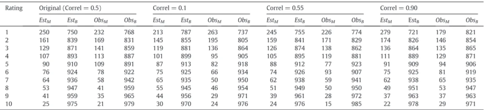
Estimated/observed values in ratings for different correlations.

Rating Original (Correl = 0.0) Correl = 0.1 Correl = 0.55 Correl = 0.90

EstM EstB ObsM ObsB EstM EstB ObsM ObsB EstM EstB ObsM ObsB EstM EstB ObsM ObsB

1 276 724 260 740 286 714 263 737 341 659 230 770 400 600 178 822 2 165 835 191 809 167 833 191 809 190 810 168 832 216 784 145 855 3 124 876 130 870 124 876 150 850 136 864 136 864 151 849 140 860 4 98 902 120 880 97 903 91 909 103 897 115 885 112 888 119 881 5 80 920 68 932 78 922 73 927 79 921 77 923 83 917 98 902 6 65 935 62 938 62 938 65 935 61 939 100 900 62 938 82 918 7 52 948 38 962 50 950 51 949 47 953 58 942 46 954 64 936 8 41 959 39 961 39 961 52 948 34 966 52 948 32 968 57 943 9 30 970 22 978 28 972 27 973 23 977 25 975 21 979 37 963 10 17 983 17 983 15 985 23 977 11 989 15 985 10 990 28 972 Table 16

Values obtained by changing the correlation (for the model with a correlation of 0.5).

Correlation KS AUROC AR Pietra Index Brier CIER KL IV M

0.10 0.343* 0.722* 0.445* 0.121* 0.084 0.088* 0.023* 0.656* 0.762* 0.20 0.386* 0.737* 0.473* 0.13* 0.087 0.102* 0.034* 0.303* 0.733* 0.30 0.348* 0.721* 0.441* 0.123* 0.086 0.086* 0.023* 0.646 0.798 0.40 0.332 0.713 0.426 0.117 0.082 0.079 0.025 0.595 0.874 0.55 0.300 0.699 0.398 0.106 0.085 0.072 0.023 0.58 0.869 0.60 0.298 0.693 0.387 0.106 0.084 0.064 0.02 0.479 0.9 0.70 0.269* 0.668* 0.336* 0.095* 0.091* 0.049* 0.016* 0.371* 0.83 0.30 0.264* 0.677* 0.353* 0.093* 0.086 0.054* 0.017* 0.413* 0.874 0.90 0.247* 0.66* 0.321* 0.087* 0.085 0.044* 0.014* 0.345* 0.832

(11)

4.2.2. Impact caused by changes in the variance of X2

From an application of the chosen model to samples with variation of theX2variance (originally, the variance had the value 4.0), the results obtained for the validation metrics are presented inTable 8.

It is possible to observe from the results presented inTable 8that the measures are, in general, not very sensitive to changes in the variance of the independent variable, and only a major change in the variance (deviation equal to 10.00) caused the indicators to be outside the estimated conﬁdence interval. Regarding the correctness of the default values of the ratings, it is possible to observe a result consistent with other metrics, i.e., a lower correctness for the deviation of 10.00, as indicated byTable 9.

4.2.3. Impact caused by changes to the bi-stochastic matrices

The matrices initially used to associate variablesX1andX2to variable Ywere the matricesM1andM1'. These matrices had high values in their diagonals (the main diagonal in case ofX1and the secondary diagonal in case ofX2) that cause a stronger dependency relationship between independent variables and the dependent variable.Table 10presents the results of the validation techniques obtained using the chosen model for portfolios simulated using the other bi-stochastic matrices.

Based on the results presented inTable 10, it is possible to observe that all metrics except the Brier score exhibited decreased model perfor-mance as the dependency between the variables was changed. Measure

Mwas relatively insensitive to the change in dependency because its value changed less sensitively than those of other measures, such as the entropy measures (CIER,IV, andKL),KS,AUROC,Pietra, andAR. In practical terms, the metrics indicate that if the model was developed using a variable that has a strong relationship with the default event and this relationship isweakenedover time, the discriminative ability of the model will decrease. Table 11 presents the estimated and observed values for each model rating.

It is possible to observe from the information contained inTable 11

that there was no considerable change in model correctness between the original portfolio and the portfolio simulated fromM3andM3'. There was a more signiﬁcant change in model correctness for the portfolio simulated from the matricesM5andM5'. Another aspect that can be observed is that in the original model, the heterogeneity of the rate of defaults observed among the ratings is greater than in the portfolio that used the matricesM5andM5'. This greater homogeneity in default rates among ratings can be observed from the sharp drop in the value of the entropy measures among portfolios.

4.3. Portfolios with dependent variables simulated using gaussian copulas Similar to the tests conducted with independent variables, 20 portfo-lios were generated to determine a conﬁdence interval for the valida-tion techniques. However, in this case, 20 portfolios with zero correlation betweenX1andX2and 20 portfolios with a correlation of Table 17

Estimated/observed values in ratings (for the model with a correlation of 0.5).

Rating Original (Correl = 0.5) Correl = 0.1 Correl = 0.55 Correl = 0.90

EstM EstB ObsM ObsB EstM EstB ObsM ObsB EstM EstB ObsM ObsB EstM EstB ObsM ObsB

1 250 750 232 768 213 787 263 737 245 755 226 774 279 721 179 821 2 161 839 169 831 145 855 195 805 159 841 171 829 174 826 146 854 3 129 871 141 859 119 881 136 864 126 874 138 862 136 864 135 865 4 107 893 113 887 101 899 95 905 105 895 119 881 111 889 129 871 5 90 910 109 891 87 913 82 918 88 912 77 923 91 909 94 906 6 76 924 78 922 75 925 66 934 74 926 93 907 75 925 81 919 7 64 936 58 942 65 935 50 950 62 938 59 941 62 938 65 935 8 53 947 41 959 55 945 46 954 51 949 50 950 49 951 53 947 9 41 959 35 965 44 956 29 971 39 961 28 972 37 963 37 963 10 25 975 21 979 30 970 24 976 24 976 15 985 22 978 29 971

(12)

0.5 betweenX1andX2were generated.Tables 12 and 13present the mean values for each technique and the conﬁdence intervals for portfo-lios with correlations of zero and 0.5.

4.3.1. Impact caused by correlation emergence

Among the 20 models with zero correlation that were used to deter-mine the conﬁdence interval, modelDepGZero03, i.e., (KS= 0.3808, AUROC= 0.7410,AR= 0.4820,PietraIndex= 0.1346,Brier= 0.0805,

CIER= 0.1021,KL= 0.0320,IV= 0.7957,M= 0.8610) was chosen to be applied to the samples with correlation variation. The results obtain-ed for the validation techniques for the samples with correlation are presented inTable 14.

All techniques, with the exception of the Brier score, exhibited a decrease in model performance with increased correlation, which was expected because the model was developed using a portfolio for which the correlation between the variablesX1andX2was zero. The observed and estimated values for each of the ratings of some models are presented inTable 15.

Based on the results presented inTable 15, it is possible to observe a signiﬁcant drop in model correctness with increased correlation between variablesX1andX2. The heterogeneity of the default rates among the ratings also decreased, which made the entropy measures sensitive. In general, the measures indicate that a model developed with non-correlated variables that explain the default event with good performance can have its performance compromised if a correlation be-tween variables comes into existence. The increase in the correlation generated a relevant impact on model correctness. For instance, taking into consideration rating 6, the observed default rate overcame the expected default rate inN60% of cases when the correlation was 0.55. 4.3.2. Impact caused by a change in the correlation

Among the 20 models with a correlation of 0.50 that were used to determine the conﬁdence interval, model DepG0.5;13, i.e., (KS = 0.3005,AUROC= 0.6998,AR= 0.3996,PietraIndex= 0.1062,Brier=

0.0858,CIER= 0.0691,KL= 0.0224,IV= 0.5365,M= 0.8897) was

chosen to be applied to the samples with distinct correlations. The re-sults obtained for the validation techniques for these samples are pre-sented inTable 16.

Except for the Brier Score, all measures were sensitive to variations in the correlation. However, because the model was developed with a correlation of 0.5, a decrease in performance was expected if the correlation values increased or decreased. All sensitive metrics, with the exception of measureM, exhibited an increase in model per-formance as the strength of the correlation was decreased. MeasureM exhibited lower model performance for both increased and decreased correlation, although the values were outside the conﬁdence interval only for the decreased correlation. Consequently,Table 17presents the estimated and observed values of default within the ratings for the models.

According toTable 17, the model correctness decreased as the corre-lation was increased or decreased, which explains the values of measure Mfor these cases. The default rates remained heterogenous along the ratings as the correlations were increased or decreased, which explains the small_ﬂuctuation in the entropy measures. TheKS,AR,AUROC, andPietrameasures were more sensitive to the order of the subjects. Therefore, it can be concluded that although the correlation change decalibrated the probability values that the model calculates, the order of the good and bad subjects was not signiﬁcantly changed.

5. Empirical sub-samples test

In this section, we developed a methodology for testing the adequa-cy of techniques for the validation ofDPwith empirical data. The meth-odology presented inSection 3, where a numerical simulation with control over the variables (factor variablesX1,X2and the response var-iable of defaultY) is used to analyze the effects of the techniques for the validation ofDP, is useful when we try to understand the effectiveness in ideal situations. In particular, we can study the behavior of metrics due to changes in the distribution, such as when the mean, the variance, and the correlation are changed. However, the values of the input

Table 18

Effects of change in the mean ofX1for validation techniques applied to a calculated empirical distribution of defaulting companies 1950–2014.

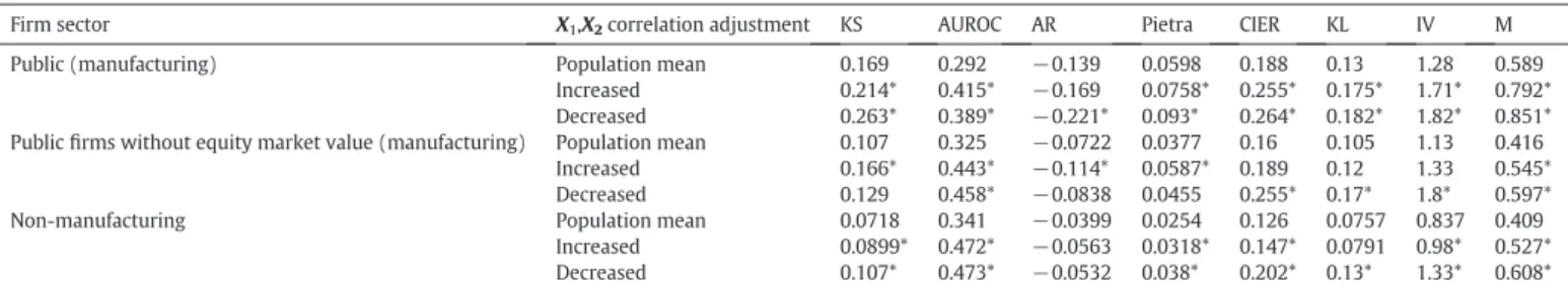
Firm sector X1mean adjustment KS AUROC AR Pietra CIER KL IV M

Publicﬁrms (manufacturing) Population mean 0.169 0.292 −0.139 0.0598 0.188 0.13 1.28 0.589

Increased 0.238* 0.4* −0.2* 0.0842* 0.275* 0.19* 1.94* 0.914*

Decreased 0.241* 0.396* −0.207* 0.0853* 0.252* 0.174* 1.68* 0.744*

Publicﬁrms without equity market value (manufacturing) Population mean 0.107 0.325 −0.0722 0.0377 0.16 0.105 1.13 0.416

Increased 0.0946 0.477* −0.0468* 0.0335 0.268* 0.186* 1.8* 0.741*

Decreased 0.171* 0.453* −0.0948 0.0604* 0.179 0.111 1.28 0.538*

Non-manufacturing Population mean 0.0718 0.341 −0.0399 0.0254 0.126 0.0757 0.837 0.409

Increased 0.102* 0.479* −0.0423 0.0361* 0.217* 0.146* 1.41* 0.658*

Decreased 0.093* 0.469* −0.0614* 0.0329* 0.14* 0.072 0.936* 0.528*

Fig. 3.Mean ofX1for good and bad borrowers of public manufacturingﬁrms, using Altman'sZ-scorefor discrimination, from January 1950 to December 2014. Source: CRSP and COMPUSTAT.

(13)

parameters used for the numerical simulation results inSection 4were not calibrated with market data; they were simply used as a numerical application of the methodology.

The purpose of this section is to provide a real-life application analysing the effects of techniques of validation for different market conditions. Comparing our analysis with that of Sobehart et al. (2000a), the contribution of this section is that we use a larger dataset and our results are provided when controlling factor variablesX1,X2 by market situations, giving the risk manager an idea of the capacity of the techniques of validation ofDPfor historical market situations. 5.1. Methodology

Thefirst part of the methodology involves defining what is a good borrower and a bad borrower. We also define the variablesX1,X2,and Y. We adopted Altman1968’s Altman1968Z-scoreto determine which companies are in distress. TheZ-score, which was initially developed for public manufacturingfirms (Altman, 1968), was extended for pri-vate_firms and non-manufacturing_firms (Altman, 2000). In these three modelsfinancial ratios with fundamental balance sheet and in-come statement data are aggregated in a discriminant analysis study to determine companies infinancial distress. There arefive ratios in the original study ofAltman (1968):

T1 Working Capital/Assets;

T2 Retained Earnings/Assets;

T3 EBIT/Assets;

T4 Market Value of Equity/Liabilities; and,

T5 Sales/Assets.

whereAssetsandLiabilitiesare totalled and the regression is given by (17), as inAltman (1968):

Z¼1:2T1þ1:4T2þ3:3T3þ0:6T4þ0:99T5; ð17Þ

This equation is used only for public manufacturing companies. The modiﬁed equation for private manufacturing companies is given by (18) as inAltman (2000):

Z¼1:7T01þ1:8T2þ3:1T3þ0:4T04þ0:99T5; ð18Þ

where:

T1 (Curr Assets - Curr Liabilities) / Assets; and T4 Book Value of Equity / Liabilities.

and for non-manufacturing and emerging market companies it is given by (19) as inAltman (2000):

Z}¼6:56T0₁þ3:26T2þ6:72T3þ1:05T04; ð19Þ

Altman (2000)found some critical values (Zb1.81 for public manufacturing, Z_b1.23 for private manufacturing, and Z_b1.1 for non-manufacturing companies). We deﬁne a bad borrower to be one with an AltmanZ-scorethat is below the critical level and otherwise it is a good borrower. The factor variables are de_ﬁned by the ratios, X1=T2,X2=T3, and the credit status isY= 1 in the event of default and zero otherwise.

Extracting theDPfrom the market data is a challenging task. As de-faults occur during the year, we model theDPusing a discrete approach, deﬁning an annualized dynamic model. Then, using an in-sample ap-proach, the distribution of defaults will be such that if the company de-faults during a year the values of the ratiosX1andX2will be associated withY= 1 and withY= 0 otherwise.

5.2. Data

The data for the defaulting companies were proxied by the informa-tion on 30,686 delisted public companies that was extracted from the CRSPdatabase and crossed with theﬁnancial fundamentals provided by theCOMPUSTATdatabase from January 1950 to December 2014. Although all the companies were public, some of them do not have

Table 19

Effects of change in the volatility ofX1for validation techniques applied to a calculated empirical distribution of defaulting companies 1950–2014.

Firm sector X1volatility adjustment KS AUROC AR Pietra CIER KL IV M

Publicﬁrms (manufacturing) Population mean 0.169 0.292 −0.139 0.0598 0.188 0.13 1.28 0.589

Increased 0.268* 0.388* −0.224* 0.0947* 0.25* 0.172* 1.65* 0.743*

Decreased 0.119* 0.475* −0.0498* 0.042* 0.27* 0.186* 1.85* 0.824*

Publicﬁrms without equity market value Population mean 0.107 0.325 −0.0722 0.0377 0.16 0.105 1.13 0.416

Increased 0.2078* 0.416* −0.169* 0.0732* 0.226* 0.134 1.8* 0.264*

Decreased 0.147 0.421* −0.159* 0.052 0.224* 0.15* 1.51* 0.568*

Non-manufacturing Population mean 0.0718 0.341 −0.0399 0.0254 0.126 0.0757 0.837 0.409

Increased 0.127* 0.453* −0.0936* 0.0448* 0.148* 0.0696* 1.03* 0.423

Decreased 0.0761 0.486* −0.0283 0.0269 0.188* 0.12* 1.22* 0.571*

Fig. 4.Volatility ofX1for good and bad borrowers of public manufacturingﬁrms, using Altman'sZ-scorefor discrimination, from January 1950 to December 2014. Source: CRSP and COMPUSTAT.