CENTER FOR MACHINE PERCEPTION CZECH TECHNICAL UNIVERSITY IN PRAGUE
PhD
THESIS
1213-2365Discriminative learning from
partially annotated examples
Kostiantyn Antoniuk
Study Programme: Electrical Engineering and Information Technology
Branch of Study: Artificial Intelligence and Biocybernetics [email protected]
CTU–CMP–2016–07
June 14, 2016
Available at
ftp://cmp.felk.cvut.cz/pub/cvl/articles/antoniuk/Antoniuk-TR-2016-07.pdf Thesis Advisors: Ing. Vojtˇech Franc, Ph.D. ,
prof. Ing. V´aclav Hlav´aˇc, CSc.
Acknowledgements: SGS15/201/OHK3/3T/13, CAK/TE01020197, UP-Driving/688652, GACR/P103/12/G084.
Research Reports of CMP, Czech Technical University in Prague, No. 7, 2016 Published by
Center for Machine Perception, Department of Cybernetics Faculty of Electrical Engineering, Czech Technical University
Discriminative learning from partially
annotated examples
Kostiantyn Antoniuk
June 14, 2016
Abstract
A number of algorithms and its applications for automatic classifiers learning from examples is ever growing. Most of existing algorithms require a training set of completely annotated examples, which are often hard to obtain. In this thesis, we tackle the problem of learning from partially annotated examples, which means that each training input comes with a set of admissible labels only one of which is correct. We contributed to two different cases of this scenario. In the first case, we studied the problem of learning the ordinal classifiers from examples with interval annotation of labels. We designed a convex learning algorithm for this case and demonstrated its advantage on real data empirically. At the same time, we made several contributions to the supervised learning of the ordinal classifiers, namely, we proposed new parametrization of the ordinal classifier, we introduced more flexible piece wise version of the ordinal classifier, and we proposed a generic cutting plane solver with convergence guarantees. In the second case, we studied the problem of learning the structured output classifiers from examples with missing annotation of a subset of labels. We have defined the concept of a surrogate classification calibrated partial loss, the minimization of which guarantees that learning is statistical consistent under fairly general conditions on the data generating process. We proved the existence of a convex classification calibrated surrogate loss for learning from partially annotated examples. We showed which existing surrogate losses are classification calibrated and which are not. Our work thus provides a missing theoretical justification for so far heuristic methods which have been successfully used in practice.
Abstrakt
Poˇcet aplikac´ı algoritm˚u pro automatick´e uˇcen´ı klasifik´ator˚u z pˇr´ıklad˚u st´ale roste. Vˇetˇsina uˇc´ıc´ıch algoritm˚u vyˇzaduje tr´enovac´ı mnoˇzinu kompletnˇe anotovan´ych pˇr´ıklad˚u, kter´e je ˇcasto teˇzk´e z´ıkat. V t´eto disertaci se zab´yv´ame probl´emem uˇcen´ı z ˇc´asteˇcnˇe anotovan´ych pˇr´ıklad˚u. ˇC´asteˇcn´a anotace znamen´a, ˇze kaˇzd´emu tr´enovac´ımu vstup je pˇriˇrazena mnoˇzina pˇr´ıpustn´ych skryt´ych stav˚u, z nichˇz pouze jedin´y je spravn´y. V disertaci popisujeme dva pˇr´ıpady patˇr´ıc´ı do tohoto sc´enaˇre. V prvn´ım pˇr´ıpadˇe jsme zkoumali uˇcen´ı ordin´aln´ıch klasi-fik´ator˚u z pˇr´ıklad˚u anotovan´ych intervalem skryt´ych stav˚u. Pro tento pˇr´ıpad jsme navrhli konvexn´ı uˇc´ıc´ı algoritmus a ovˇeˇrili jeho funkˇcnost na re´aln´ych datech. Souˇcasnˇe jsme pˇrispˇeli k ˇreˇsen´ı probl´emu uˇcen´ı ordin´aln´ıch klasifik´ator˚u z kompletnˇe anotovan´ych dat, a to konkr´etnˇe n´avrhem nov´e parametrizace ordin´aln´ıho klasifik´atoru, flexibilnˇejˇs´ım model pro ordin´aln´ı klasifikaci a obecn´ym optimalizaˇcn´ım algoritmem s garanc´ı konvergence. V druh´em pˇr´ıpadˇe jsme studovali probl´em uˇcen´ı strukturn´ıch klasifik´ator˚u z pˇr´ıklad˚u s chybˇej´ıc´ı anotac´ı u podmnoˇziny skryt´ych stav˚u. Definovali jsme pojem n´ahradn´ı klasifikaˇcnˇe kalibrovan´e ˇc´asteˇcn´e ztr´atov´e funkce, jej´ıˇz minimalizace zaruˇcuje, ˇze uˇcen´ı je statisticky konzistentn´ı za dosti obecn´ych podm´ınek na proces generuj´ıc´ı data. Dok´azali jsme, ˇze existuje konvexn´ı kalibrovan´a n´ahradn´ı ztr´atov´a funkce pro uˇcen´ı z ˇc´asteˇcnˇe anotovan´ych pˇr´ıklad˚u. Uk´azali jsme, kter´e z existuj´ıc´ıch n´ahradn´ıch ztr´atov´ych funkc´ı jsou kalibrovan´e, a kter´e nejsou. Naˇse pr´ace tak doplˇnuje chybˇej´ıc´ı teoretick´e od˚uvodnˇen´ı pro doposud heuristick´e metody ´uspˇeˇsnˇe pouˇz´ıvan´e v praxi.
Acknowledgement
I am thankful to my two supervisors Ing. Vojtˇech Franc, Ph.D. and prof. Ing. V´aclav Hlav´aˇc, CSc. for fruitful discussions and brilliant ideas which led me in my research towards the fulfillment of the Ph.D. degree.
I am grateful that I was a summer intern at Google Inc. Z¨urich in 2014. Although I am not allowed to give details due to Non-Disclosure Agreement (NDA), it was a source of great experience.
I gratefully acknowledge that my research was supported by the Technology Agency of the Czech Republic under Project TE01020197 Center Applied Cybernetics and Automated Urban Parking and Driving under Project 688652 funded by the European Union’s Horizon 2020, the Grant Agency of the CTU under the projects SGS15/201/OHK3/3T/13 and the Grant Agency of Czech Republic under project GACR/P103/12/G084.
I hereby certify that the results presented in this thesis were achieved during my own research in cooperation with my thesis advisors Ing. Vojtˇech Franc, Ph.D. and prof. Ing. V´aclav Hlav´aˇc, CSc.
Contents
Contents viii
Abbreviations 1
Symbols 1
1. Introdution 4
1.1. Discriminative learning from fully annotated examples . . . 6
1.2. Discriminative learning from partially annotated examples . . . 10
1.3. Thesis goals . . . 12
1.4. Contributions . . . 12
1.4.1. Learning ordinal classifier from interval annotations . . . 12
1.4.2. Learning structured output classifier from examples with missing labels 13 1.5. Thesis outline . . . 14
2. State-of-the-art 15 2.1. Development of the statistical consistency of learning methods . . . 15
2.1.1. Statistical consistency of the supervised flat classifiers . . . 15
2.1.2. Statistical consistency of the supervised ordinal classifiers . . . 16
2.1.3. Statistical consistency of the supervised structured output classifiers . 16 2.1.4. Statistical consistency of the flat classifiers learned from partially an-notated examples . . . 16
2.2. Existing methods for structured output learning from partial annotations . . 17
2.2.1. Convex concave procedure. . . 17
2.2.2. Regularized bundle methods for convex and non-convex risks . . . 17
2.2.3. Branch and bound algorithm . . . 18
2.2.4. Perceptron-like algorithms . . . 18
2.3. Ordinal classification . . . 18
2.3.1. Maximum likelihood methods for learning of ordinal classifier . . . 19
2.3.2. Discriminative methods for supervised learning of ordinal classifiers . 19 3. Learning ordinal classifiers from interval annotations 20 3.1. The model . . . 21
3.1.1. Ordinal regression as linear multi-class classification . . . 21
3.1.2. Piece-wise ordinal regression classifier . . . 23
3.1.3. Unified view of classifiers for ordinal regression . . . 24
3.2. Supervised learning. . . 26
3.2.1. Support vector ordinal regression: explicit constraints on thresholds . 27 3.2.2. Support vector ordinal regression: implicit constraints on thresholds . 28 3.2.3. Generic learning algorithm for ordinal regression . . . 29
3.3.1. Learning by minimizing the interval insensitive loss. . . 31
3.3.2. Interval insensitive support vector ordinal regression: explicit constraints on thresholds . . . 34
3.3.3. Interval insensitive support vector ordinal regression: implicit constraints on thresholds . . . 34
3.3.4. V-shaped interval insensitive loss minimization algorithm . . . 35
3.4. Generic cutting plane solver . . . 37
3.5. Experiments. . . 39
3.5.1. Compared methods. . . 39
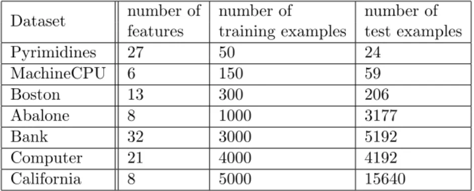
3.5.2. Benchmark data . . . 40
3.5.3. Experimental protocol . . . 41
3.5.4. Comparison of surrogate losses for supervised learning . . . 42
3.5.5. Impact of the regularization term. . . 46
3.5.6. Testing flexibility of the PW-MORD model . . . 46
3.5.7. Learning from interval annotations . . . 48
3.5.8. Tightness of the upper bound on the Bayes risk . . . 48
3.5.9. Comparison of surrogate losses for learning from interval annotations. 48 3.5.10. Equivalence between SVOR-IMC and VILMA-MAE . . . 49
3.6. Conclusions . . . 49
4. Statistical consistency of structured output learning with missing labels 57 4.1. Supervised learning of structured output classifiers . . . 57
4.2. Minimization of the partial loss . . . 59
4.3. Statistical model of partial annotations. . . 60
4.4. Consistency of the partial loss . . . 62
4.5. Classification calibrated surrogates of the partial loss . . . 64
4.6. Existence of the convex surrogate for partial loss . . . 65
4.7. Examples of surrogate losses. . . 66
4.8. Relation to existing works . . . 69
4.9. Conclusions . . . 70
5. Conclusions and open questions 71 A. Proofs 73 A.1. Proof of Theorem 1. . . 73
A.2. Proof of Theorem 3. . . 75
A.3. Proof of Proposifion 1 . . . 75
A.4. Proof of Proposition 2 . . . 76
A.5. Proof of Theorem 4. . . 76
Bibliography 80 A. Author’s publications 86 A.1. Publications related to the thesis . . . 86
Impacted journal papers excerpted by ISI . . . 86
Conference papers excerpted by ISI . . . 86
A.2. Other publications . . . 86 Impacted journal papers excerpted by ISI . . . 86 Impacted journal papers not excerpted by ISI . . . 86
Abbreviations
ACCPM Analytic Center Cutting Plane Method . . . .39
BMRM Bundle Method for Risk Minimization . . . .17
CCCP Convex-Concave Procedure. . . .17
CPA Cutting plane algorithm . . . .20
CRF Conditional Random Field . . . .16
ERM Empirical Risk Minimization . . . .5
II-SVOR-EXP Interval-Insensitive SVOR-EXP . . . .34
II-SVOR-IMC Interval-Insensitive SVOR-IMC. . . .34
LP Linear Programming . . . .18
LinCls Linear Multi-class SVM classifier . . . .39
LinReg Rounded linear regressor . . . .39
MAE Mean Absolute Error . . . .26
MORD Multi-class Ordinal classifier . . . .13
NBMRM Non-Convex Bundle Method for Risk Minimization . . . .17
PW-MORD Piece-Wise Multi-class ORDinal classifier . . . .13
QP Quadratic Programming . . . .37
SO-SVM Structured Output Support Vector Machine . . . .13
SVOR-EXP Support Vector Ordinal Regression: Explicit Constraints on Thresholds . . . . .19
SVOR-IMC Support Vector Ordinal Regression: Implicit Constraints on Thresholds . . . . .19
SVR Support Vector Regression . . . .31
Symbols
X Instance space x Instance Y Label space Y Labeling space y Discrete label y Labeling w Weight vectorArgmin The set of all minimizers of function argmin Single minimizer of function
h Classifier, a mapping from the instance space to the label space
` Original loss function
ψ, variants Surrogate loss functiton
pred Predictor mapping from the surrogate space to the label space
R`, variants Risk induced by a loss function `
[[A]] is the Iverson bracket. It evaluates to 1 if Aholds, otherwise it is 0.
h·,·i Dot product
Dm
xy Dataset with fully annotated examples
Dm
xI Dataset with interval-annotated examples
Dm
Failure is an option here. If things are not failing, you are not innovating enough.
1. Introdution
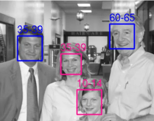
In this thesis, we consider a problem of learning classifiers from partially annotated examples. This means that instead of a single label per instance, we are given a set of admissible labels only one of which is correct. Such scenario is common in practice. For instance, the problem of learning from partially annotated examples naturally arises in age recognition from facial images. Instead of acquiring a precise age for each facial image in the training set, which is often expensive or impossible, it is easier to collect age ranges that can be, for example, estimated by a human annotator. See Figure1.1where each subject is annotated by a range of ages instead of a precise age. Another motivating application can be image segmentation as illustrated in Figure 1.2. Obtaining a ground true label for each pixel in the image is obviously tedious and expensive, therefore very often we are provided with an incomplete labeling, meaning that some pixels in the training image are left unannotated.
To put the problem of learning from partial annotations into perspective, it is useful to list other common learning scenarios (see also Figure1.3):
• In thesupervised scenario each training instance is annotated with a single label.
• In theunsupervised scenario training instances have no label at all.
• In the semi-supervisedscenario each training instance either has a single label or it has no label at all.
• In themulti-instancescenario training instances are not individually labeled but grouped into sets, which either contain at least one positive example or only negative examples.
• In thepartially annotatedscenario, i.e. the scenario analyzed in this thesis, each training instance is annotated with a set of admissible labels only one of which is correct.
There exists two standard paradigms that have been used for learning from partially an-notated examples: the generative approach and the discriminative approach. The generative approach tries to model the joint probability distribution of the input observations and the labels. To this end, one has to select an appropriate class of probabilistic models. As soon as the class of the probabilistic models is chosen, the maximum likelihood method (or other
Figure 1.1. Example of facial images with partial annotation of age. Getting rough age ranges of each person is relatively easy while providing exact age is difficult.
(a) (b) (c)
Figure 1.2. An example of a training instance when learning structured output classifier for image segmentation task. Example of an input image (a), a good(complete) labeling (b), coarse (partial) labeling (c). instance label (a)supervised instance ??? (b)unsupervised instance instance label ??? (c)semi-supervised instance instance instance label (d)multi-instance instance label label label (e)partial-label
Figure 1.3. Different learning scenarios (figure adopted from [Cour et al.,2011]).
estimation method) is used to select a single model best fitting to the training data. Finally, the required classification rule is inferred from the learned probabilistic model. On the other hand, the discriminative approach tries to learn the classification rule directly. To this end, one has to select an appropriate class of classification rules. Once the classification model is chosen, the Empirical Risk Minimization (ERM) principle (or other method) is used to select a single classification rule best fitting to the training data.
In this thesis, we follow the discriminative approach. The existing discriminative methods for learning from partially annotated examples often suffer from the following problems: 1. There is no clear connection between the target objective and the objective function actually
optimized by the learning algorithm. The target objective is typically the expectation of the complete loss which evaluates the response of the classifier given the ground truth label. The objective function of the learning algorithm is typically an average of a “partial loss” computed on the partially annotated examples. The partial loss is a certain function which evaluates the response of the classifier given the partial annotation.
2. The learning problem is usually transformed into a non-convex minimization problem which is then approached by a local optimization method with no certificate of optimality. During our work, we were mainly focused on these two problems. In short, our main contributions are the following:
• (Ad problem 1) We developed tools which allow to analyze the statistical consistency of algorithms learning the structured output classifiers from partially annotated examples. Here the partial annotation means that a subset of output labels describing the training
1. Introdution
instance is missing, e.g. like in the image segmentation examples show in Figure 1.2. We applied the proposed methodology to existing ad-hoc algorithms and we showed which of them are statistically consistent and which are not. Loosely speaking, the consistent algorithm provides a minimizer of the target objective, i.e. the expectation of the complete loss, provided the number of partially annotated training examples goes to infinity. That is, we built a missing bridge between the objective function of the consistent algorithms and the target objective.
• (Ad problem 2) We introduced a new partial loss applicable for learning the ordinal clas-sifiers from examples with the interval annotation of the labels, e.g. like in the example shown in Figure 1.1. We establish a connection between the proposed partial loss and an associated complete target loss. We designed a convex surrogate of the partial loss which allows to convert learning into an optimization problem which can be solved efficiently and we show how to do it by cutting plane methods. As a byproduct we made several contributions to the supervised learning of the ordinal classifiers, namely, we proposed new parametrization of the ordinal classifier and we introduced more flexible piece wise version of the ordinal classifier.
In the following two sections we briefly describe the ERM based learning algorithms. We first outline the standard supervised scenario and then the scenario with the partially anno-tated examples. We use the two sections in order to introduce a notation which allow us to describe goals and contributions of the thesis more precisely at the very end of this chapter.
1.1. Discriminative learning from fully annotated examples
Let us briefly describe supervised learning algorithms based on the ERM principle. The supervised algorithms require a set of completely annotated training examples
Dm
xy ={(x1, y1), . . . ,(xm, ym)} ∈(X × Y)m (1.1) typically assumed to be drawn from independent and identically distributed (i.i.d.) random variables with some unknown distribution p(x, y). The symbol X denotes a set of input observations and Y is a set of labels to be predicted. In this thesis we assume that Y is finite. The goal of the supervised learning is formulated as follows. Given a loss function
`:Y × Y →R+ and the training examples (1.1), the task is to learn the classifier h:X → Y
whoseBayes risk(the target objective)
R`(h) =Ep(x,y)`(y, h(x)) (1.2)
is as small as possible, i.e. ideally, we would like to obtain the best Bayes classifier1
h`
∗∈Argmin
h:X →Y
R`(h). (1.3)
The minimization problem (1.3) cannot be solved directly due to the unknown distribution
p(x, y). The ERMprinciple approaches the problem (1.3) by the following approximations: 1Strictly speaking one has to consider inf
h:X →YR
`(h) here, however, in order to make the main message clear
we assume that infimum is reachable and we can use minimum instead. Later, in Chapter 4, we describe our contribution in the strict way using infimums.
1.1. Discriminative learning from fully annotated examples • The empirical distribution
s(x, y) = 1 m m X i=1 [[xi =x∧yi =y]] (1.4) is used instead of the true but unknown distribution p(x, y).
• The set of all possible classifiers h:X → Y is restricted to some predefined set of rulesH (the hypothesis space).
Using these approximations, the ERMamounts to solving
hemp∗ ∈Argmin
h∈H
Remp` (h), (1.5) where
Remp` (h) =Es(x,y)`(y, h(x)) (1.6) is the empirical risk andhemp∗ is the learned classification rule. Under certain conditions [
Vap-nik, 1995], the ERM is statistically consistent learning algorithm, i.e. for the number of examples going to infinity the expected risk of the learned classifier R`(hemp
∗ ) converges in
probability to the minimal Bayes riskR`(h`
∗).
Unfortunately even simple instances of theERMproblem (1.5) are hard to solve efficiently and thus it is further simplified in the following way. The original loss function`:Y ×Y →R+ is replaced by a surrogate loss functionψ:Y ×T →ˆ R operating on a surrogate decision set
ˆ
T ⊂RY. With the help of the surrogate loss functionψwe learn a surrogate decision function
f:X →Tˆ, which is then used to construct the decision functionh:X → Y via a predefined transform pred : ˆT → T, i.e. h = pred◦f. As before, the set of all surrogate decision functionsf:X →Tˆ is restricted to a subsetF. With these changes, theERMproblem (1.5) is simplified to a search for the the best surrogate decision function by solving
f∗emp ∈Argmin
f∈F
Rempψ (f), (1.7) where
Rψemp(f) =Es(x,y)ψ(y, f(x)) (1.8) and the resulting classification rule is h = pred◦f∗emp. The surrogate loss function ψ is
typically chosen to be a convex function that upper bounds the original loss `. The convex surrogate loss makes the problem (1.7) convex and much easier to deal with than the original problem (1.5). Besides the convexity, however, the used surrogate loss should have a clear statistical meaning. A natural requirement is to use such surrogate losses which preserves the statistical consistency of theERM principle.
Loosely speaking, if a given surrogate loss ψ:Y ×T →ˆ R is so called classification cali-brated [Ramaswamy and Agarwal,2012] (or statistically consistent [Zhang,2004a,b], or Fisher consistent [Shi et al.,2015]) with respect to the original loss `:Y × Y → R+ then it holds that
pred◦f∗ψ ∈Argmin
h:X →Y
R`(h) (1.9)
for any distributionp(x, y), where
f∗ψ ∈Argmin
f:X →Tˆ
1. Introdution
and
Rψ(f) =
Ep(x,y)ψ(y, f(x)) (1.11) is the expectation of the surrogate loss. In words, using a classification calibrated surrogate guarantees that a solution of the surrogate problem (1.10) is a decision function f∗ψ which
defines a classification ruleh = pred◦f∗ψ being itself a minimizer of the original task (1.9).
In practice the distribution p(x, y) is unknown and thus we do not minimize the surrogate riskRψ(f) but rather its empirical estimateRψ
emp(f). However, it can be still shown that the classification calibrated surrogate preserves the statistical consistency of theERM.
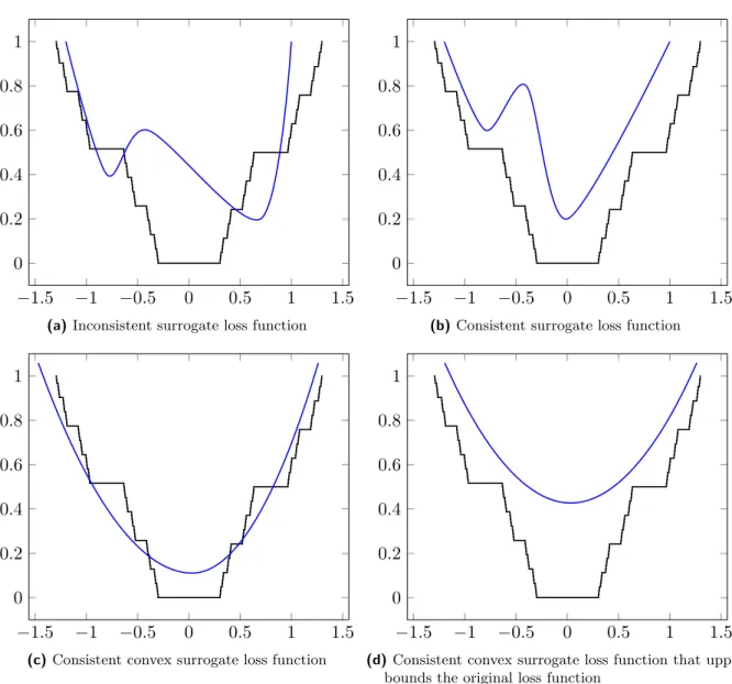
It should be emphasized that the classification calibrated surrogate loss does not have to be an upper bound of the target loss `:Y × Y → R+ since the inclusion in (1.9) is required for the minimizers of the surrogate loss. Of course, an analysis of the minimizers is often more difficult and hence, it is common in practice to deal with surrogate losses that are upper bounds of the target loss. See Figure 1.4for illustration.
Example. Let us consider learning of a multi-class linear classifier. A surrogate decision function is learned from a set of linear functions
F =
f(x) = (hw1,xi,· · · ,hwY,xi)T |(w1, . . . ,wY)∈Rn×Y,kw1k2+· · ·+kwYk2≤λ with parameters whose Euclidean norm is bounded byλ > 0. Each f ∈ F maps an input
x∈ Rn onto t∈ T ⊂ˆ RY. The classification rule is constructed by composing the decision functionf with a transform pred(t),argmax
y∈Y
ty so that the resulting classification rule reads
h(x) = pred◦f(x) = argmax y∈Y
fy(x) = argmax y∈Y h
wy,xi.
For example, the multi-class Support Vector Machine algorithm learns the decision function
f by solving the problem (1.7) with different surrogate loss functions used in practice: 1. A commonly used surrogate
ψ(ˆy, f(x)) = max
y∈Y(1 +fy(x)−fyˆ(x))
is not statistically consistent w.r.t. to the target 0/1-loss`(ˆy, y) = [[ˆy6=y]], unless we deal only with those distributions p(x, y) such that∃y∈ Y, p(y|x)> 12 ([Liu,2007]).
2. In contrast, less commonly used surrogate loss
ψ(ˆy, f(x)) =X y6=ˆy
max(0,1 +fy(x)−fyˆ(x))
is consistent with respect to the target 0/1-loss`(ˆy, y) = [[ˆy6=y]] ([Liu,2007]).
The statistical consistency of theERMbased fully supervised learning algorihtms have been intensively studied. Unfortunately, it is not possible to directly apply all the existing results in the case of partially annotated examples. In the next section we are going to explain main issues which raise when we apply the ERM methods to the partially annotated examples.
1.1. Discriminative learning from fully annotated examples −1.5 −1 −0.5 0 0.5 1 1.5 0 0.2 0.4 0.6 0.8 1
(a)Inconsistent surrogate loss function
−1.5 −1 −0.5 0 0.5 1 1.5 0 0.2 0.4 0.6 0.8 1
(b)Consistent surrogate loss function
−1.5 −1 −0.5 0 0.5 1 1.5 0 0.2 0.4 0.6 0.8 1
(c)Consistent convex surrogate loss function
−1.5 −1 −0.5 0 0.5 1 1.5 0 0.2 0.4 0.6 0.8 1
(d)Consistent convex surrogate loss function that upper bounds the original loss function
Figure 1.4. The figure illustrates different cases of the surrogate loss and the target loss function. For some fixedp(x, y),x∈ X andy∈ Y, we plot the value of original loss as`(y,pred◦f(x)) and the surrogate loss asψ(y, f(x)). The x-axis corresponds tof ∈ F and the y-axis shows the value of the target loss`(y,pred◦f(x)) shown in black and the surrogate lossψ(y,pred◦f(x)) shown in blue.
1. Introdution
1.2. Discriminative learning from partially annotated examples
In the case of learning from partially annotated examples, we are provided with a set of admissible labels only one of each is correct. This differs from the supervised setting, where we have one to one correspondence between the input instances and labels. More precisely, we consider a set of partially annotated training examplesDxam ={(x1,a1), . . . ,(xm,am)} ∈(X ×2Y)m, (1.12) assumed to be drawn from i.i.d. random variables with some unknown joint distribution
p(x,a) =X y
p(x,a, y).
Each training input xi comes along with a set of candidate labels ai ⊂ 2Y ( |a| ≥ 1). A
common assumption on the data generating distribution p(x,a, y) is that the ground truth labelyi is among the known candidate labels ai, i.e. yi ∈ai.
The ultimate goal is the same as in the supervised learning, that is, for a given loss function
`:Y × Y →R+ we want to learn a classifierh:X → Y whose Bayes risk (1.2) defined w.r.t
p(x, y) =X a
p(x,a, y)
is as small as possible. Although the goals are the same, the learning algorithms are not. Namely, theERMmethodology cannot be used directly because the loss function`:Y × Y →
R+is undefined over the annotations (i.e. the subsets 2Y) contained in the partially annotated training set Dm
xa. One option to make the ERM applicable is to derive so called partial loss
`P:Y ×2Y →
R+ from a given complete (target) loss`by minimizing over admissible labels:
`P(y,a) = min ˆ
y∈a`(ˆy, y). (1.13) The partial loss`P has been explicitly defined in [Cour et al.,2011] for a case when` is the 0/1-loss. However implicitly, via defining a learning algorithm which in its core minimizes the partial loss, it has been used many times in various contexts. For example, it is minimized by an algorithm learning the Hidden Markov Chain based classifiers [Do and Arti`eres,2009], generic structured output models [Lou and Hamprecht,2012], the multi-instance learning [Luo and Orabona,2010] or the named entity recognizer [Fernandes and Brefeld,2011a].
Having the partial loss, we can define the partial risk
R`P(h) =Ep(x,a)`P(h(x),a), (1.14) and search for the best (Bayes) classifierh:X → Y that minimizes the partial risk
h`∗P ∈Argmin
h:X →Y
R`P(h). (1.15) The partial risk minimization problem (1.15) can be already approached by theERMmethods. However, the central question is whether theERMmethods can provide a good approximation of the target problem (1.3). An answer to this question in the case of structured output classification (i.e. wheny is a vector of labels) is one of the contributions of the thesis. Our approach is very briefly outlined in the rest of this section.
1.2. Discriminative learning from partially annotated examples
We will show that for some distributionsp(x,a, y) the problem (1.15) is equivalent to the target problem (1.3) in the sense that both problems share the set of solutions. In particular, the classifierh`P
∗ obtained by minimizing the partial risk (1.15) is a minimizer of the target
(complete) risk (1.2) as well, i.e. the inclusion
h`P ∗ ∈Argmin h:X →Y R`(h) (1.16) holds or equivalently R`(h`∗P) =R`(h`∗). (1.17)
After establishing the equivalence (1.17), one can solve the partial risk minimization prob-lem (1.15) by the ERMmethods as follows. The partial risk (1.14) can be approximated by the empirical risk
R`empP (h) =Es(x,a)`P(h(x),a), (1.18) where s(x,a) = 1 m m X i=1 [[xi =x∧ai=a]]. (1.19) As in the supervised setting, the partial empirical risk (1.18) is hard to minimize directly. Hence, the partial loss`P:Y ×2Y →
R+is replaced by an easier-to-minimize surrogate partial lossψP: 2Y
×T →ˆ R+, which operates on the surrogate decision set ˆT ⊂RY. The surrogate
ψP loss is used to learn a surrogate decision functionf:X →Tˆ such that
f∗emp,ψp ∈Argmin f∈F RψempP (f), (1.20) where RψP emp(f) =Es(x,a)ψP(a, f(x)). (1.21) Finally, the resulting classification rule is constructed by composing the learned function
f∗emp,ψp and a fixed prediction function pred, i.e. h= pred◦femp,ψ
p
∗ .
Likewise in the supervised setting, in order to justify theERMproblem (1.20) we also need to study consistency of the surrogate partial loss. To this end, we introduce in this thesis a concept of a classification calibrated partial loss. Loosely speaking, if a surrogate partial loss
ψp is classification calibrated w.r.t. the partial loss `p then for any distributions p(x,a) it holds that
pred◦f∗ψP ∈Argmin h:X →Y
R`P(h), (1.22) wheref∗ψP is a minimizer of the partial surrogate risk, i.e.,
f∗ψP ∈Argmin
f:X →Tˆ
RψP(f), (1.23)
RψP(f) =Ep(x,a)ψP(a, f(x)). (1.24) Consequently, using the inclusion (1.20) we can show that any minimizer of the partial sur-rogate riskf∗ψP is the Bayes classifier of the target (complete) risk, i.e., it holds that
pred◦f∗ψP ∈Argmin
h:X →Y
1. Introdution
In this sense the minimization of the surrogate partial riskRψP
(f) is equivalent to (or consis-tent with) the minimization of the target riskR`(h). Under some conditions, the equivalence is preserved even if the true risks are replaced by their empirical estimates. This allows us to show that the learning algorithms which in their core solve the problem (1.20) with calibrated surrogate partial loss are statistically consistent. Namely, we will prove that for the number of examples going to infinity the expected risk of the learned classifier R`(pred◦femp,ψp
∗ )
converges in probability to the minimal (Bayes) riskR`(h`
∗).
1.3. Thesis goals
This thesis is centered around the ERM based algorithms learning classifiers from partially annotated examples. More precisely, we concentrated on learning algorithms which in their core solve the surrogate ERM problem (1.20). At the beginning of our work on this topic, there were many ad-hoc methods showing that algorithms implementing (1.20) give promising results, i.e. they were shown to provide a good approximations of the Bayes classifier (1.3). However, there was no firm theory which would support these empirical findings. In addition, the existing algorithms often suffer from using a non-convex surrogate partial losses making the problem (1.20) hard to optimize. And thus a further question is in which cases one can construct a good convex and, at the same time, easy-to-optimize surrogate partial loss. After recognizing the open problems, we focused our work on the following questions:
• How to design a convex surrogate of the partial loss (1.13)?
• How to solveERM problem (1.20) efficiently?
• Under which conditions are algorithms implementing ERM problem (1.20) statistically consistent?
We have not found a complete and general answer to these questions, yet we managed to contributed to all of them. A summary of our contributions is provided in the next section.
1.4. Contributions
In this work, we investigated two different classification scenarios both falling under the um-brella of learning from partial annotations. First, learning of ordinal classifiers from interval annotations. Second, learning of structured output classifiers from examples with missing labels.
1.4.1. Learning ordinal classifier from interval annotations
We consider learning of the ordinal classifiers (i.e. classification model assuming ordered labels) from examples of inputs annotated by intervals of admissible labels.
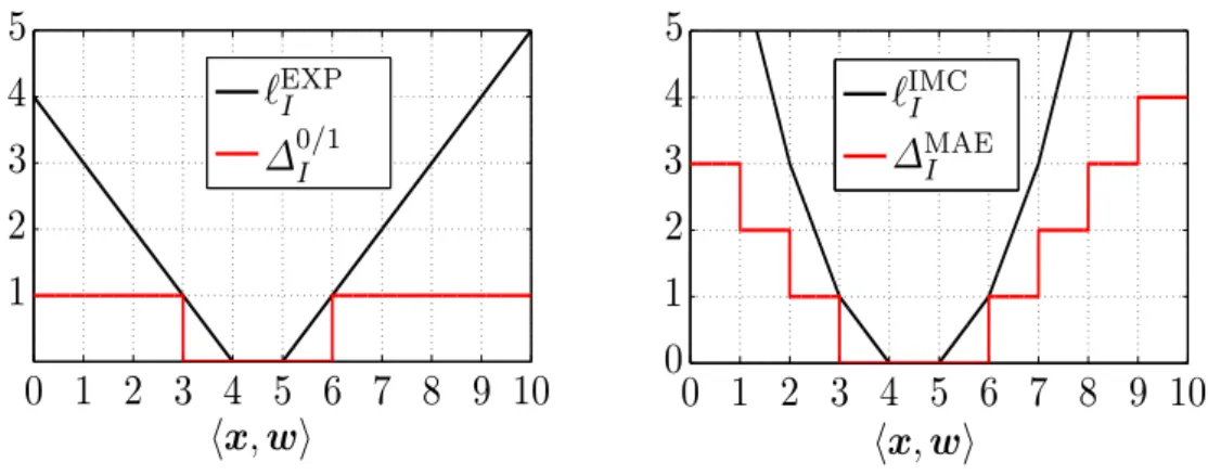
• We propose an interval insensitive loss (IIL) function to measure discrepancy between the interval of admissible labels given in the annotation and a label predicted by the classifier. The IIL can be build from arbitrary target (complete) V-shape loss like, for example, the 0/1-loss or mean absolute error (MAE). The IIL is an instance of the generic partial loss (1.13). In contrast to existing instances of the partial loss (1.13), the IIL for ordinal classification can be approximated by tight convex surrogates as we will show.
• We show that the expectation of the IIL is a reasonable proxy of the expectation of the target complete loss. In particular, we show that the target risk R` is upper bounded by
1.4. Contributions
a linear function of the partial risk R`P
. We show how the tightness of this upper bound depends on the annotations process which was used to generate the training examples.
• We show how to build tight convex surrogates of the IIL. The convex surrogates are obtained by extending surrogates known from existing supervised algorithms for ordinal regression. These surrogates are can be used as a proxy for the 0/1-loss or the MAE loss. We also propose a novel convex surrogate of a generic V-shaped interval-insensitive loss.
• We propose an efficient cutting plane solver for minimization of theERMproblem (1.20). In contrast to existing CPA solvers, it can deal with situations when the quadratic regularizer is not imposed on all model parameters which, as will be also shown, has significant influence on the final accuracy of the learned ordinal classifier.
• We have not managed to prove consistency of the IIL. Instead, we performed a thorough empirical evaluation showing that minimization of the interval insensitive loss provides a good approximation of the target Bayes classifier (1.3).
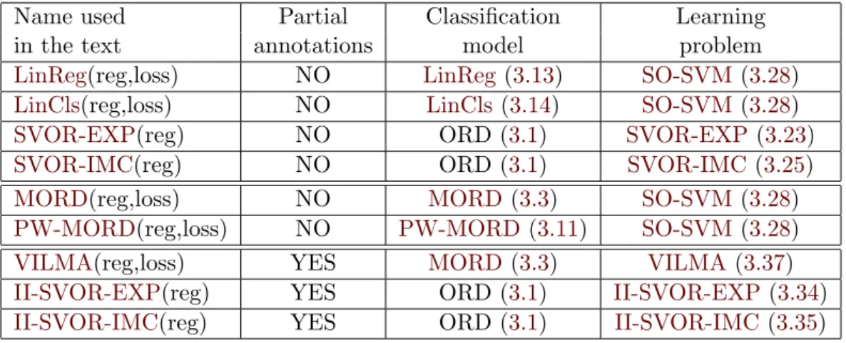
While working on this topic, we also made some progress on supervised learning of ordinal classifiers as a byproduct:
• We proved that the ordinal classifier is equivalent to a linear multi-class classifier whose class parameter vectors are collinear and with magnitude linearly increasing with the labels. We call the new representation as the Multi-class Ordinal classifier (MORD) classifier. Our equivalence proof is constructive so that we can convert any ordinal classifier to theMORD classifier and vice-versa.
• The MORD representation allows to express the space of ordinal classifiersHord as compo-sition of the “argmax” prediction transform pred(t) = argmaxy∈Yty and a linear decision function f ∈ F, i.e. Hord ={pred◦f |f ∈ F}. In turn, the MORD representation can be beneficial for learning and analysis of the ordinal classifiers by using algorithms and results for well understood multi-class linear classification. For example, we show that a generic Structured Output Support Vector Machine (SO-SVM) algorithm can be applied for learning of theMORDclassifier and that it delivers the same (or slightly better) results when compared to the existing learning algorithms for the ordinal classification. Moreover, the SO-SVM approach works for arbitrary loss function in contrast to existing methods which require the V-shaped losses.
• We show that theMORDrepresentation allows introduce more complex models for ordinal classification. Namely, we propose a Piece-Wise Multi-class ORDinal classifier (PW-MORD) which subsumes the standard ordinal classifier and unrestricted multi-class classifies as spe-cial cases. We demonstrate advantages of the proposed models on standard benchmarks as well as on solving a real-life problem of estimating human age from facial images.
1.4.2. Learning structured output classifier from examples with missing labels We concentrate on a scenario, when the object is characterized by an input observation and labelling of a set of local parts, however, a training set contains examples of inputs and labelings only for a subset of the local parts.
• We provide sufficient conditions which admit to prove that the expected riskR`(h) of the structured predictorhlearned by minimizing the partial riskR`P
(h) converges in probabil-ity to the optimal Bayes risk R`(h`
∗). The sufficient conditions restrict the target loss `to
be additive over the local parts while the data generating process p(x,a,y) can be fairly generic.
1. Introdution
• We define a concept of classification calibrated surrogate partial losses which are easier to optimize, yet their minimization preserves the statistical consistency.
• We analyze surrogate losses used by the existing algorithms implementing theERM min-imization (1.20) for learning of structured output classifiers from examples with missing labels. For example, we show that the ramp-loss and some of its modifications which have been most frequently used are classification calibrated and, in turn, the corresponding algo-rithms are statistically consistent. Our analysis provides a missing theoretical justification for so far heuristic methods.
• We prove the existence of a convex classification calibrated surrogate for partial learning. The proof is based on establishing a connection between learning from partially annotated examples and the recently published theory on consistency of supervised learning.
1.5. Thesis outline
Chapter 2 contains the state-of-the-art relevant to the topics studied in the thesis. In
particular, we review works related to the statistical consistency of algorithms learning from fully annotated and partially annotated examples, we also review optimization algorithms which have been used to solve the ERM problem (1.20) and, finely, we review existing discriminative learning methods for the ordinal classifiers.
Chapter 3 describes our contributions to the problem of learning ordinal classifiers from
fully annotated examples and examples with interval (partial) annotation of labels.
Chapter 4 describes our contributions to the problem of statistical consistency of
algo-rithms learning structured output classifiers from examples with missing labels.
Chapter 5 contains conclusions resulting from the work done in this thesis and also a
discussion of a possible future work.
2. State-of-the-art
2.1. Development of the statistical consistency of learning
methods
Undisputably, the consistency of a learning method is a desirable property, i.e. a good learn-ing method should recover the Bayes classifier at least if provided with an infinitely large training set under the condition that the class of considered classifiers contains the Bayes classifier. The design of consistent learning methods for supervised multiclass prediction re-ceived the attention in the last decade: [Zhang,2004b,a;Bartlett et al.,2006;Hill and Doucet,
2007;Tewari and Bartlett,2007;Liu,2007;Santos-Rodr´ıguez et al.,2009;Zhang et al.,2009;
Ramaswamy and Agarwal, 2012]. Statistical properties of learning algorithms based on the risk minimization formulation are relatively well-understood for the supervised setting due to the aforementioned works and others. However, there are quite few works studying risk based minimization methods for the learning setting with the missing labels. Among the few exceptions belong the works of [Cour et al.,2011;Cid-Sueiro et al.,2014;Yu et al.,2014]. 2.1.1. Statistical consistency of the supervised flat classifiers
[Zhang, 2004b] showed first that binary classifiers obtained by minimizing infinite-sample consistent surrogate loss for supervised learning (e.g. the hinge-loss, logistic loss, etc.) can approach Bayes classifier. [Zhang, 2004a] analysed the consistency of the hinge loss and its modifications in the context of the multiclass classification formulations such as pairwise com-parison, constrained comparison and One-Versus-All methods. [Liu,2007] considered several multiclass generalizations of the hinge-loss used in various multiclass SVMs algorithms and showed that some of them were and others were not statistically consistent. For some incon-sistent losses, [Liu,2007] showed how to modify training algorithm to make the losses behave consistently. [Tewari and Bartlett,2007] characterized classification calibration of supervised multiclass problems in terms of geometric properties of some sets associated with the sur-rogate loss function. Based on these properties, they provided certain sufficient conditions for the classification calibration and examine the consistency of a few multiclass methods. [Ramaswamy and Agarwal, 2012] extended the notion of the classification calibration from 0/1-loss and/or binary classification problems to the general multiclass setting with a gen-eral loss. [Ramaswamy and Agarwal, 2012] deriveed necessary and sufficient conditions for a surrogate loss function to be classification calibrated with respect to a given target loss. They introduced the notion of so called convex classification calibration dimension of a mul-ticlass loss matrix measuring the size of a prediction space, in which it is possible to design a convex surrogate that is calibrated with respect to the target loss. They derived lower and upper bounds of the classification calibration dimension as well. These notions can be very useful if for a given target loss one has to prove existence or non-existence of a corresponding convex calibrated surrogate loss. The consistency of multiclass losses were also considered in the development of various types of other settings, e.g. the multiclass classification with
re-2. State-of-the-art
ject option [Ramaswamy et al.,2015a], hierarchical classification [Ramaswamy et al.,2015b], multiclass boosting [Zhu et al.,2009;Mukherjee and Schapire,2013], etc.
2.1.2. Statistical consistency of the supervised ordinal classifiers
[Pedregosa et al., 2014] studied the statistical consistency of methods used for supervised ordinal classifier learning of rich family of surrogate loss functions including proportional odds and support vector ordinal regression. Authors consider the threshold and the regression based models for which they derived sufficient conditions on statistical consistency for the margin based methods and the surrogates of the V-shape loss functions. In Section 3.3, we will extend the notion of V-shaped surrogate losses for dealing with interval annotations. 2.1.3. Statistical consistency of the supervised structured output classifiers Although there is a progress in studying the supervised multiclass setting for flat classifiers, there are only few works dedicated directly to the structured output prediction. [Shi et al.,
2015] investigated the relationship between the classification calibration of multiclass losses and losses for a structured output prediction in supervised scenario. They proposed a hybrid loss for supervised multiclass and structured output problems that is a convex combination of a logarithmic loss for Conditional Random Field (CRF) and a multiclass hinge loss from the SVM methods. Their family of losses is similar to those proposed previously by [Zhang et al.,
2009] for 0/1 loss. [Shi et al., 2015] provided a condition for a given loss to be statisticaly consistent for classification, which depends on a measure of dominance between labels, i.e. the gap between probabilities of the best labeling and the second best labeling. They showed that the statistical consistency is necessary also for so called parametric consistency which is needed when learning models such as theCRFs.
2.1.4. Statistical consistency of the flat classifiers learned from partially annotated examples
The literature on consistency of supervised learning methods is rich. The consistency of meth-ods learning from partially annotated examples has been addressed very rarely so far. We are aware only of two works addressing the problem, namely [Cour et al.,2011] and [Cid-Sueiro et al., 2014]. [Cour et al., 2011] considered the multiclass learning of flat classifiers from examples with candidate set of admissible labels. They proposed a convex learning formula-tion based on a minimizaformula-tion of a certain partial loss. They also analyzed condiformula-tions under which their partial loss is asymptotically consistent against the target 0/1 loss. [Cid-Sueiro et al.,2014] proposed a generic framework which, for a given supervised target loss, allows to derive a classification calibrated surrogate suitable for learning from training examples with missing labels. Authors introduced a statistical model under which they show that consistent surrogate losses for learning with missing labels can be obtained by a linear transformation of any surrogate consistent loss for the supervised setting. Authors showed that convexity can be sometimes preserved when adapting a supervised surrogate loss to its weak consistent counterpart.
Although the setting studied in [Cour et al.,2011;Cid-Sueiro et al.,2014] is quite general, (they considered any subset of labels as candidate label set), neither of them can be used to analyze existing methods learning the structured output classifiers, i.e. the multiclass clas-sification with exponentially large number of labels. Their convex surrogate losses designed
2.2. Existing methods for structured output learning from partial annotations
for flat classifiers are not suitable for structured case since their evaluation requires solving computationally intractable subproblems.
Nevertheless, part of the community drops the statistical part of the problem and tries to solve the problem using ad-hoc heuristics that give very often reasonably good results in practice. For the sake of completeness, we give a brief overview of existing approaches below.
2.2. Existing methods for structured output learning from partial
annotations
Most of the following works try to contribute to the practical part of the problem by improving existing heuristics for solving the non-convex ERM task (1.20) in a context of particular application. We provide a short overview of optimization methods used in the structured output learning from partially annotated examples.
2.2.1. Convex concave procedure
Many different approaches assuming that the minimization of the partial empirical risk to be good estimate have beed proposed during last decade [Chuong et al., 2008; Girshick et al.,
2011; Yu and Joachims, 2009; Fernandes and Brefeld, 2011a; Zhu et al., 2010; Vedaldi and Zisserman,2009;Wang and Mori,2010;Luo and Orabona,2010;Lou and Hamprecht,2012;
Sarawagi and Gupta,2008;Yu et al.,2014]. Most of these works derived a non-convex bound on the partial empirical risk (1.14) and proved empirically that it gives good estimates in various types of applications. Non-convex optimization problems trying to solve (1.20) are reduced to a sequence of convex problems, by so called Convex-Concave Procedure (CCCP), which reduces the non-convex problem into a sequence of convex ones. Convex subproblems are often solved with the help of proximal bundle method [Kiwiel, 1990]. Most of proposed improvements forCCCPconsist of:
• An adaptive increasing of the precision of supervised problem on eachCCCPiteration until the required precision is reached. This reduces the number of gradient evaluations needed for Bundle Method for Risk Minimization (BMRM) on eachCCCPiteration.
• Reusing “good” cutting planes across multiple CCCP iterations and avoiding computing them from the scratch.
Different kind of CCCP ’s improvement was proposed by [Kumar et al., 2010], so called Self-Paced Learning. Their algorithm simultaneously selects easy examples and updates pa-rameters on each iteration in order to escape local optima. The number of samples selected at each iteration is determined by a weight that is gradually annealed so that later iterations introduce more samples. The algorithm convergences after all samples have been considered and the objective function can not be improved further.
2.2.2. Regularized bundle methods for convex and non-convex risks
[Do and Arti`eres,2012] adapted the convex solverBMRM [Teo et al.,2010] for non-convex optimization problem. The main idea of the Non-Convex Bundle Method for Risk Minimiza-tion (NBMRM) is, likewise inBMRM, to build an approximation of the partial surrogate loss via the cutting plane technique iteratively. Such an approximation is not an underestimator of the objective function anymore, since the objective function is no more convex. The cutting plane approximation of the objective function may cause conflict with target function, i.e. it
2. State-of-the-art
may lead to the overestimation of the objective function at certain points. Authors overcome the conflicts between the cutting planes similarly to classical non-convex bundle methods [ Ki-wiel,1985; Gaudioso and Monaco, 1992] and prove the global convergence to cluster points which are stationary solutions (not necessarily a local minimum but may be a saddle point or even a local maximum). Their method requires fine tuning of many hyper-parameters, which makes the algorithm very sensitive for each particular application.
2.2.3. Branch and bound algorithm
[Kawahara and Washio,2011] used branch and bound algorithm for structured output learning problems with missing labels known in global optimization theory [Horst et al.,1991]. Instead of difference of two convex functions, authors considered submodular functions, the discrete analog of convex functions. In addition, instead of solving Linear Programming (LP) problem needed for computing a lower bound in a continuous case, authors solved binary-integer linear program using state of the art optimization techniques developed for the optimization of submodular functions. Authors showed empirically the advantage of the model corresponding to the global optimum of objective function over the models corresponding to local optima. Although, the branch and bound algorithm is not really suitable for large scale problems, it shows the advantage of the global solution against the local one in the considered approach (structured output learning from partially annotated data).
2.2.4. Perceptron-like algorithms
The structured output perceptron, analogous to its “flat” counterpart, has been proposed in [Schlesinger and Hlav´aˇc,2002; Altun et al.,2003; Collins and Koo,2005]. Later [Fernandes and Brefeld, 2011b] derived an extension of the loss-augmented perceptron for structured output learning that allows to deal with partialy annotated sequences. To learn from partialy annotated data [Fernandes and Brefeld,2011b], performed a transductive step to extrapolate the partial annotations to the unlabeled part using the constrained Viterbi algorithm [Cao and Chen,2003]. The perceptron-like algorithms have a clear advantage, namely, that they are an online type of algorithms suitable for learning from large scale data. The main disadvantage of such algorithms is an incomplete theoretical understanding like the convergence analysis (in turn it is unclear when to stop the algorithm) or a firm statistical justification [Fernandes and Brefeld,2011b]. Nevertheless, most of the existing works show empirically that minimization of the partial loss function when learning the structured output classifiers from missing labels is a good heuristic.
2.3. Ordinal classification
First it should be mentioned that there is a plethora of works in machine learning community addressing supervised learning of ordinal classifiers. However, there is a lack of discriminative methods for learning from partially annotated examples. The existing approaches are briefly discussed below.
The ordinal classification models can be split to two groups: a regression based approaches and a threshold based approaches. The former approach involves the standard regression model the real-valued output of which is then projected on a discrete domain corresponding to the ordinal labels [Crammer and Singer,2005]. On the other hand, the threshold based
2.3. Ordinal classification
approaches provide a greater flexibility by seeking a mappingf:X →R along with a vector of non-decreasing thresholds which partition the real-valued prediction into an ordered set of labels. The existing learning paradigms can be split into two groups as well: the maximum likelihood based methods and the discriminative methods which are briefly outlined below. 2.3.1. Maximum likelihood methods for learning of ordinal classifier
A plug-in ordinal classifier can be constructed by substituting a probabilistic model estimated by the ML method to the optimal decision rule derived for a particular loss function (see e.g. [Debczynski et al.,2008] for a list of losses and corresponding decision functions suitable for ordinal classification). Parametric probability distributions suitable for modeling the ordinal labels have been proposed in [McCullagh, 1980;Fu and Simpson, 2002; Rennie and Srebro,2005]. Besides the parametric methods, the non-parametric probabilistic approaches like the Gaussian processes were also proposed [Chu and Ghahramani,2005].
The maximum likelihood approach can be directly applied in the presence of incomplete an-notation (e.g. the setting considered in this work when label interval is given instead of a single label) by using the Expectation-Maximization algorithms [Schlesinger,1968;Dempster et al.,
1997]. However, the maximum likelihood methods are sensitive to model mis-specification which complicates their application in modeling complex high dimensional data. In con-trast, the discriminative methods reviewed below are known to be robust against the model misspecification while their extension for learning from partial annotations is not trivial. 2.3.2. Discriminative methods for supervised learning of ordinal classifiers
The existing discriminative methods learn parameters of the ordinal classifier by minimizing a convex proxy of the empirical risk. A Perceptron-like on-line algorithm PRank has been pro-posed in [Crammer and Singer,2001]. A large-margin principle has been applied for learning ordinal classifiers in [Shashua and Levin,2002]. The paper [Chu and Keerthi,2005] proposed Support Vector Ordinal Regression: Explicit Constraints on Thresholds (SVOR-EXP) and the Support Vector Ordinal Regression: Implicit Constraints on Thresholds (SVOR-IMC). Unlike [Shashua and Levin, 2002], the SVOR-EXP and SVOR-IMC guarantee the learned ordinal classifier to be statistically plausible. The same approach have been proposed inde-pendently by [Rennie and Srebro, 2005], who introduce so called immediate-threshold loss and all-thresholds loss functions. Minimization of a quadratically regularized immediate-threshold loss and the all-immediate-threshold loss are equivalent to theSVOR-EXPand theSVOR-IMC formulation, respectively. A generic framework proposed in [Li and Lin,2006], of which the SVOR-EXPand SVOR-IMC are special instances, allows to convert learning of the ordinal classifier into learning of two-class SVM classifier with weighted examples.
3. Learning ordinal classifiers from interval annotations
A road map of the chapter:
• Classification models for ordinal classification are discussed in Section 3.1. In
Subsec-tion 3.1.1 we show that the standard ordinal rule can be equivalently parametrized as a specific form of a linear multi-class classifier, which we denote as the MORD classifier. In Subsection 3.1.2 we propose a more flexible model for ordinal classification which we denoted as thePW-MORD classifier. A unified view of existing and proposed models for ordinal classification is presented in Subsection 3.1.3.
• Supervised learningalgorithms for ordinal classification are discussed in Section3.2. Two
existing methods, the support vector ordinal machine with explicit constraints (SVOR-EXP) and the support vector ordinal machine with implicit constraints (SVOR-IMC) [Chu and Keerthi,2005], are reviewed in Subsection3.2.1and Subsection3.2.2, respectively. In Sub-section 3.2.3 we show how to design an instance of the SO-SVM which can learn ordinal classifiers while minimizing a surrogate of an arbitrary V-shaped loss.
• Learning from interval annotationsis discussed in Section3.3. The interval-insensitive
loss function and its application as an upper bound of the target (complete) loss is a subject of Subsection3.3.1. Modifications of two existing supervised methods, the SVOR-EXP and the SVOR-IMC algorithms, in order to minimize a surrogate of the interval-insensitive loss is presented in Subsection 3.3.2 and Subsection3.3.3, respectively. A generic surrogate of the interval-insensitive loss which can be derived from arbitrary V-shaped loss is proposed in Subsection3.3.4. In Subsection3.3.4we also propose an instance of a genericERMbased algorithm, called V-shaped interval insensitive loss minimization algorithm (VILMA), and we discuss its relation to other methods.
• Optimization algorithm that is suitable for solving large instances of the convex
prob-lems formulated in this chapter is proposed in Subsection3.4. The algorithm, denoted as a double-loop Cutting plane algorithm (CPA), can solve convex quadratically regularized risk minimization problems. In contrast to existing instances of the CPA, the double-loop CPA allows a subset of parameters not to be included in the quadratic regularizer which is very important when modeling the intercepts of the ordinal classification rules as will be shown experimentally.
• Experimentsare presented in Section3.5. The experiments provide a thorough evaluation
of the supervised methods and the methods for learning from interval annotations discussed in this chapter. The evaluation is carried out on both standard UCI benchmarks as well as on a real-life problem the goal of which is the estimation of human age from facial images.
3.1. The model 1 1 1 1 1 1 3 2 2 2 2 2 3 3 3 3 3 4 4 4 4 4 4
θ
1θ
2θ
3h
w, x
i
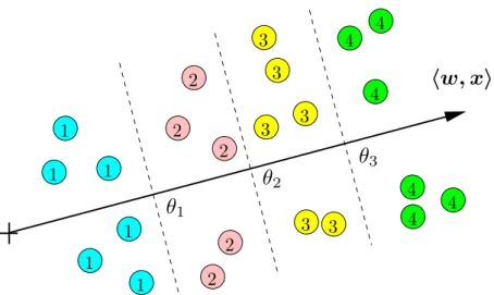
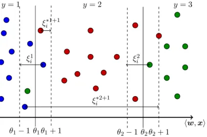
Figure 3.1. The figure vizualizes division of the 2-dimensional feature space into four classes realized by an instance of the ordinal classifier (3.1).
3.1. The model
Let X ⊂ Rn be a space of input observations and Y = {1, . . . , Y} a set of hidden labels endowed with a natural order1. We consider learning of an ordinal classifierh:X → Y of the
form h(x;w,θ) = 1 + Y−1 X k=1 [[hx,wi> θk]], (3.1) where w ∈ Rn and θ ∈ Θ = {θ0 ∈ RY−1 | θ0y ≤ θy+10 , y = 1, . . . , Y −1} are admissible parameters. The brackets h·,·i denote the dot product and the operator [[A]] is the Iverson bracket. It evaluates to 1 if Aholds, otherwise it is 0. The classifier (3.1) splits the real line of projectionshx,wiintoY consecutive intervals defined by thresholdsθ1 ≤θ2≤ · · · ≤θY−1.
The observationx is assigned a label corresponding to the interval, to which the projection
hw,xifalls to. The classifier (3.1) is a suitable model if the label can be thought of as a rough measurement of a continuous random variableξ(x) =hx,wi+ noise [McCullagh, 1980]. An example of the ordinal classifier applied to a toy 2D problem is depicted in Figure3.1.
We define an equivalent parametrisation of an ordinal classifier in the next section. 3.1.1. Ordinal regression as linear multi-class classification
Let us start with one-dimensional observationsx∈ X =R. In such case the ordinal classifier
h(x) = 1 +PYk=1−1[[x > θk]] splits the real axis intoY intervals defined by thresholdsθ1 ≤θ2≤
· · · ≤θY−1. One may think of representing the ORD classifier in the form
h0(x) = argmax y∈Y
f(x, y), (3.2)
wheref: R× Y →R is a discriminant function. If we manage to construct the discriminant functions such that f(x, y) > f(x, y0), y0 ∈ Y \ {y} iff h(x) = y then both representations
1The sequence 1, . . . , Y is used just for a notational convenience. However, any other finite and fully ordered set can be used instead.
3. Learning ordinal classifiers from interval annotations
θ1 θ2
2x+b2 3x+b3
x+b1
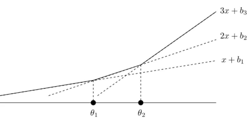
Figure 3.2. The figure illustrates the relation between the ordinal classifierh(x) = 1 +PY−1
k=1[[x > θk]]
and its alternative representation h0(x) = argmaxy∈Y(x·y+by) for the (Y = 3)-class problem.
Note, thatxandy-axes have different scale in order to save space.
will be equivalent i.e. h0(x) = h(x), x ∈ R. Let us consider a linear discriminant function with the slope equal to y, i.e. f(x, y) = x·y +by. In such case (3.2) becomes a linear multi-class classifier. It is not difficult to see that such linear classifier also splits the real axis into intervals. Figure 3.2shows an example of the ordinal classifier and its equivalent linear classifierh0(x).
The same idea can be applied forn-dimensional observationsx∈ X =Rn. The multi-class linear classifier which can represent the ordinal classifier (3.2) reads
h0(x;w,b) = argmax y∈Y hx,wi ·y+by , (3.3)
wherew∈Rnis the parameter vector andb= (b1, . . . , bY)∈RY is a vector of intercepts. We denote (3.3) as the Multi-class Ordinal classifier (MORD). Later in this text, we assume that the “argmax” operator returns the minimal label in the case of more than one maximizer.
A natural question is whether both representations are equivalent in the sense that any ordinal classifier can be represented by someMORD classifier and vice-versa. The following theorem gives the positive answer to the question.
Theorem 1. The ordinal classifier (3.1) and the MORD classifier (3.3) are equivalent in
the following sense. For any w ∈ Rn and admissible θ ∈ Θ there exists b ∈ RY such that
h(x,w,θ) =h0(x,w,b),∀x∈Rn. For any w∈Rnand b∈Rn there exists admissible θ∈Θ
such thath(x,w,θ) =h0(x,w,b),∀x∈Rn.
Our proof (see AppendixA.1) is constructive in the sense that we can provide a conversion from the ordinal classifier to theMORDclassifier and vice-versa.
In exotic cases, which however may appear in practice, some classes can collapse to a single point and effectively disappear. To cover all such situations, we first define the concept of non-degenerated classifier and then we give formulas for the conversions.
Definition 1(Degenerated and non-degenerated classifier). We call classy∈ Y non-degenerated
for classifier h0(x) iff Xy = interior({x ∈ X : h0(x) = y}) 6= ∅. Classifier h0(x) is
non-degenerated iff all classes are non-non-degenerated. In the opposite case, the classifier is called degenerated.
3.1. The model
Definition 2. Given a MORD classifier, the class yˆ ∈ Y is non-degenerated iff the linear
inequalities
zyˆ+byˆ> z(ˆy−k) +byˆ−k, 1≤k <y ,ˆ
zyˆ+byˆ≥z(ˆy+t) +by+kˆ , 1< t≤Y −y ,ˆ
(3.4)
are solvable w.r.t. z∈R.
Note that the validity of (3.4) can be verified in O(Y) time. The proof of Theorem 1 can be found in Appendix A.1. The proof is a constructive, i.e., it provides formulas which allow to convert the MORD classifier (3.3) to the standard ordinal classifier (3.1) and vice-versa.
Conversion formulas. Given parameters of the ordinal classifierw∈Rn, θ∈Θ, the equiv-alentMORD classifier has parametersw and bgiven by
b1 = 0 and by =− y−1
P i=1
θi, y= 2, . . . , Y. (3.5) The conversion from theMORD classifier to the ordinal classifier is done differently for the non-generated and the degenerated classifier. Given parameters of a non-degeneratedMORD classifier w ∈ Rn and b ∈ RY, we can compute thresholds θ ∈ Θ of the equivalent ordinal classifier by
θy =by−by+1, y= 1, . . . , Y −1. (3.6) Given parameters of a degenerated MORD classifier w ∈ Rn and b ∈ RY, we compute thresholds θ∈Θ of the equivalent ORD classifier by
θyi =· · ·=θyi+1−1 =
byi−byi+1
(yi+1−yi), i= 1, . . . , p, (3.7)
whereyi ∈ Y, i= 1, . . . , pis an increasing subsequence of non-degenerated classes.
Finally, let us note that the MORD classifier is represented by n+Y parameters insted of n+Y −1 parameters of the ordinal classifier. However, the parameters of the MORD classifier are unconstrained, which makes the MORD representation attractive for learning because no additional constraints on the interceptsθ∈Θ are needed.
3.1.2. Piece-wise ordinal regression classifier
The discriminative power of the ordinal classifier can be limiting in some cases. Mapping the observations into higher dimensional space via usage of kernel functions is one way to make the linear ordinal classifier more discriminative. Though the “kernalization” of the ordinal classifier is straightforward it is not suitable in all cases. For example, the kernels are prohibitive in applications, which require processing of large amounts of training examples and/or if a real-time response of the classifier is the must. Instead, we proposed to stay in the original feature space where we construct a combined classifier from a set of simpler component classifiers. In our case, the component classifiers will be the MORD classifiers, each responsible for a subset of labels.
Let Z >1 be a number of cut labels (ˆy1,yˆ2, . . . ,yˆZ) ∈ YZ such that ˆy1 = 1, ˆyZ = Y and ˆ
3. Learning ordinal classifiers from interval annotations
Yz ={y ∈ Y |yˆz ≤y≤yˆz+1},z∈ Z. We will model a dependence between the observation
x and a subset of labelsYz by the component classifier
hz(x) = argmax y∈Yz
fz(x, y), (3.8)
where fz:Rn× Yz → R is a discriminant function. We define a combined classifier whose discriminant function is composed of discriminant functions of the component classifiers as follows h00(x) = argmax z∈Z max y∈Yz fz(x, y). (3.9)
We set the discriminant functions to be
fz(x, y) = x,wz(1−α(y, z)) +wz+1α(y, z) +by, (3.10) where α(y, z) = y−yˆz ˆ yz+1−yˆz
and W = [w1, . . . ,wZ] ∈ Rm, b ∈ RY, (where m = n×Z) are parameters. With these definitions, it can be claimed that:
1. the component classifiers (3.8) are the ordinal classifiers,
2. the combined classifier (3.9) is well defined because all its neighboring discriminant functions are consistent at the cut labels, i.e. fz(x,yˆz+1) =fz+1(x,yˆz+1),z∈ Z, holds.
The claim 1 is seen after substituting (3.10) into (3.8), which after some algebra yields
hz(x) = argmax y∈Yz hx,wz+1−wziα(y, z) +by .
Sinceα(y, z) is linearly increasing withy, Theorem 1 guarantees thathz(x) is theMORD clas-sifier equivalent to the ordinal clasclas-sifier. The claim 2 follows from the fact thatα(ˆyz+1, z) = 1 andα(ˆyz+1, z+ 1) = 0, and thus fz(x,yˆz+1) =hx,wz+1i+byˆz+1 =fz+1(x,yˆz+1).
We can write explicitly the component classifier, which we call thePW-MORD, as follows
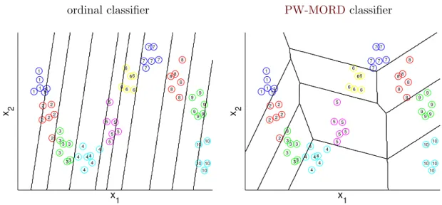
h00(x,W,b) = argmax z∈Z argmax y∈YZ hx,wz(1−α(y, z)) +wz+1α(y, z)i+by . (3.11) Figure 3.3 visualizes the ordinal (=MORD) and the PW-MORD classifier on a toy data. It is seen that the distribution of the data cannot be well described by the ordinal classifier, while the PW-MORD composed of three ordinal classifiers provides much better model in this case.
3.1.3. Unified view of classifiers for ordinal regression
In this section, we are going to describe several instances of the classifier
h(x,W,b) = argmax y∈Y hx, Z X z=1 β(y, z)wzi+by , (3.12)
where W = [w1, . . . ,wZ] ∈ Rn×Z, b = [b1;. . .;bY] ∈ RY are parameters and β: Y ×
{1, . . . , Z} → R are fixed numbers, that can be useful models for ordinal regression. The instances of (3.12) differ in the way how one definesβ and Z. We show below how to derive various instances of the ordinal classifier.
3.1. The model
ordinal classifier PW-MORDclassifier
1 11 1 1 1 2 2 2 2 2 2 3 3 3 33 3 3 4 4 4 4 4 4 4 5 5 5 5 5 5 6 6 66 66 7 7 7 7 7 7 8 8 8 8 8 8 9 9 9 99 9 10 10 10 10 10 x 1 x 2 1 11 1 1 1 2 2 2 2 2 2 3 3 3 33 3 3 4 4 4 4 4 4 4 5 5 5 5 5 5 6 6 66 66 7 7 7 7 7 7 8 8 8 8 8 8 9 9 9 99 9 10 10 10 10 10 x 1 x 2
Figure 3.3. The figure shows the partitioning of 2-dimensional feature space realized by the ordinal classifier and thePW-MORDclassifier withZ= 3 components. The cut labels for thePW-MORD
classifier were set to{1,4,7,10}.
1. Rounded linear-regression rule
h(x,w, b) = max(1,min(Y,round(hw,xi+b))) (3.13) is the most simplest model for the ordinal regression obtained by clipping a rounded response of the standard linear regression rule to the interval [1, Y]. It is easy to show that (3.13) is an instance of (3.12) recovered after setting Z = 1, β(1, y) = 2y, y ∈ Y, and fixing the components of the intercept vector bto by = 2by−y2. Using the conversion formula (3.6), we can show that the rounded linear-regression rule is equivalent to the ordinal classifier with equal width of the decision intervals, namely, with θk+1−θk = 2,k= 1, . . . , Y −2.
2. Multi-class linear classifier
h(x,W,b) = argmax y∈Y h
wy,xi+by
(3.14) is recovered after setting Z =Y and β(y, z) = [[y =z]], y∈ Y,z ∈ {1, . . . , Z}. It is the most generic (and also most discriminative) form of (3.12), which completely ignores ordering of the labels.
3. The proposed MORD classifier (3.3) is recovered after setting Z = 1, W = w1, and
β(y,1) =y,y∈ Y. We showed that theMORDclassifier is equivalent to the standard ordinal classifier (3.1) most frequently used in the ordinal regression.
4. The proposed PW-MORD classifier (3.11) is recovered after setting β(y, z) according to
β(y, z) = 1−α(y, z) for z= 1, . . . , Z−1, y ∈ Yz,
β(y, z) = α(y, z−1) for z= 2, . . . , Z , y∈ Yz,
β(y, z) = 0 otherwise.
![Figure 1.3. Different learning scenarios (figure adopted from [Cour et al., 2011]).](https://thumb-us.123doks.com/thumbv2/123dok_us/9901688.2483564/17.892.146.759.425.616/figure-different-learning-scenarios-figure-adopted-cour-et.webp)