Context-FOFE Based Deep Learning Models for Text Classification and Modeling

(1)

CONTEXT-FOFE BASED DEEP LEARNING MODELS FOR TEXT CLASSIFICATION AND MODELING

YUPING LIN

A THESIS SUBMITTED TO THE FACULTY OF GRADUATE STUDIES IN PARTIAL FULFILMENT OF THE REQUIREMENTS

FOR THE DEGREE OF MASTER OF SCIENCE

GRADUATE PROGRAM IN

ELECTRICAL ENGINEERING AND COMPUTER SCIENCE YORK UNIVERSITY

TORONTO, ONTARIO AUGUST 2017

c

(2)

Abstract

Text classification is a fundamental task in natural language processing. Many recently proposed deep learning models have leveraged context information in docu-ments and achieved great successes. However, most of these models use complicated recurrent structures to handle the variable-length text and to record context infor-mation, which are hard to train. In this case, we propose a simple and efficient encoding scheme called context-FOFE that can encode context of variable-length documents into fixed-size representations. Our encoding is unique and reversible for any text sequence. Based on the encoded representations of documents, we further use two feed-forward neural network models and a generative HOPE model for text classification and modeling. We tested the models on the 20 Newsgroups text classification dataset and the IMDB sentiment analysis dataset. Experimental results show that our models can achieve competitive performance as the existing best models while using much simpler context encoding mechanism and network structure.

(3)

Acknowledgements

Foremost, I would like to express my sincere gratitude to my advisor Prof. Hui Jiang for his continuous support through my Master study and research. His motivation, enthusiasm and immense knowledge are what I admired and encourage me to keep on studying. I also deeply appreciate his patience and valuable guidance helping me in both research and writing this thesis.

I would also like to express my gratitude to all the professors who taught me during my undergraduate and graduate study at York University, for the knowledge and help they gave me during my study.

I am especially thankful to York University and the department of computer science for their support and providing all the facilities to enrich my graduate study experience.

My special thanks also goes to my parents. Their understanding, support and encouragement give me the opportunity to pursue my degree.

(4)

for Neural Computing and Machine Learning (iNCML) at York University who assisted me in research and writing this thesis. I have learned a lot from many discussions with them.

(5)

List of Tables

6.1 Summary of the 20 Newsgroups dataset . . . 73 6.2 Performance of position-wise trained FNNs on different tasks. . . . 94 6.3 Performance of document-wise trained FNNs on different tasks. . . 94 6.4 Performance of comparative HOPE models on different tasks. . . . 94 6.5 Performance comparison with existing models. . . 95 6.6 Performance comparison with the bag-of-words based FNN model. . 96

(9)

List of Figures

2.1 Commonly used activation functions. . . 17

2.2 Typical structure of feed-forward neural networks (FNN). . . 19

2.3 Typical structure of convolutional neural networks (CNN). . . 20

2.4 Typical structure of recurrent neural networks (RNN). . . 21

2.5 Illustration of the back-propagation mechanism. The blue arrow denotes the forward direction of information flow, and the red arrows denotes the direction of the error back-propagation. . . 26

2.6 Graphical model representation of LDA. The boxes are ”plates” rep-resenting replicates. The outer plate represents documents, while the inner plate represents the repeated choice of topics and words within a document. (This figure is from [4]). . . 29

2.7 Structure of the recurrent convolutional neural network (RCNN). (This figure is from [22]). . . 32

(10)

2.8 Structure of the one-hot bidirectional LSTM with pooling model (oh-2LSTMp). (This figure is from [20]). . . 34

3.1 Illustration of the FOFE encoding scheme. . . 38 3.2 Context-FOFE encoding scheme. (a) Context around wordwt. Words

are represented as one-hot vectors. (b) Context matrix. The context vectors are of the same size. . . 41

4.1 Structure of position-wise trained FNN. B denotes the mini-batch size; V denotes the vocabulary size;D denotes the word embedding dimension and C denotes the number of classification categories. . . 50 4.2 Voting strategies for context-FOFE based FNNs. Ldenotes the

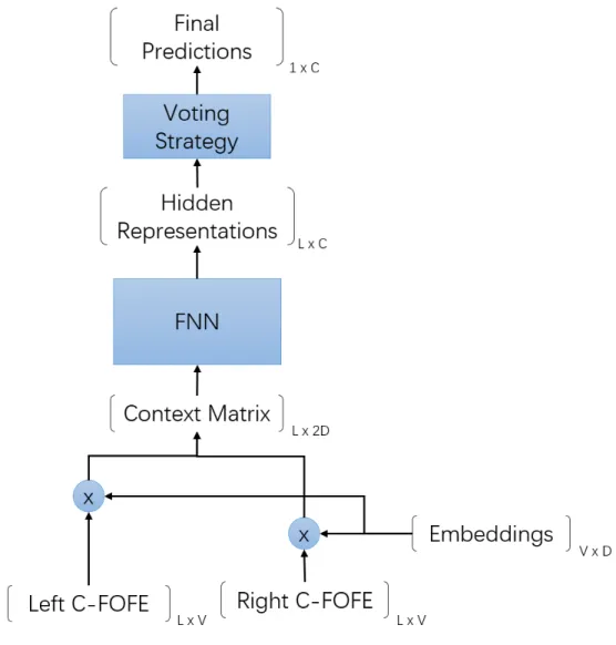
doc-ument length. . . 53 4.3 Structure of document-wise trained FNN. L denotes the document

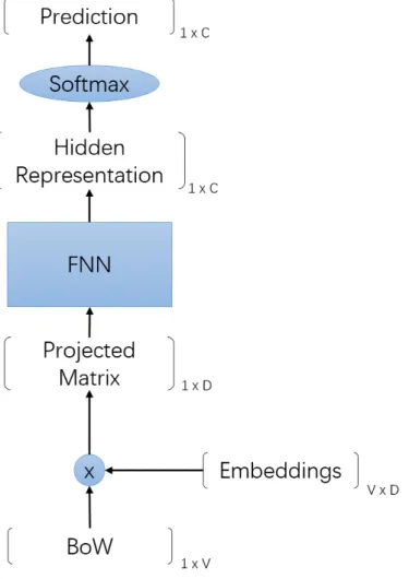
length; V denotes the vocabulary size; D denotes the word embed-ding dimension and C denotes the number of classification categories. 56 4.4 Structure of bag-of-words based FNN.V denotes the vocabulary size;

Ddenotes the word embedding dimension andCdenotes the number of classification categories. . . 58

(11)

5.2 The comparative evaluation strategy of HOPE models. . . 70

6.1 Effects of different word embeddings on the performance of the position-wise trained model. . . 80 6.2 Effects of different vocabulary size on the performance of the

position-wise trained model for the IMDB dataset. . . 81 6.3 Effects of different forgetting factor on the performance of the

position-wise trained model. . . 82 6.4 Effects of different voting strategy on the performance of the

position-wise trained model. . . 83 6.5 Effects of different mini-batch size on the performance of the

document-wise trained model on the 20 Newsgroups 4 categories task. . . 85 6.6 Effects of different mini-batch size on the performance of the

document-wise trained model on the 20 Newsgroups 20 categories task. . . 86 6.7 Effects of different mini-batch size on the performance of the

document-wise trained model on the IMDB task. . . 87 6.8 Effects of different voting strategy on the performance of the

document-wise trained model. . . 88 6.9 Effects of differentM on the performance of the comparative HOPE

(12)

6.10 Effects of different K on the performance of the comparative HOPE model. . . 92 6.11 Effects of different forgetting factor on the performance of the

(13)

Abbreviations

BoW Bagof Words

BPTT Back-PropagationThrough Time CNN Convolutional Neural Network CPU Central Processing Unit

EM Expectation-Maximization (algorithm) FNN Feed-forward Neural Network

FOFE Fixed-size Ordinally Forgetting Encoding GPU Graphics Processing Unit

HOPE Hybrid Orthogonal Projection and Estimation LDA Latent Dirichlet Allocation

LSTM Long Short-Term Memory (network) MLE Maximum Likelihood Estimation NLP Natural Language Processing NN Neural Network

(14)

PCA PrincipleComponent Analysis

RCNN Recurrent Convolutional Neural Network ReLU RectifiedLinear Unit

RNN Recurrent Neural Network SGD Stochastic Gradient Descent SVM Support Vector Machine SWE Semantic Word Embedding vMF von Mises-Fisher (distribution)

(15)

1 Introduction

Text classification (or text categorization) is an important task in Natural Lan-guage Processing (NLP) that aims to automatically assign natural lanLan-guage text documents to predefined categories according to their content. In terms of a clas-sification problem, the task is defined as follow. Given a set of N training samples

X ={x1, . . . , xN}, with each of them associated with a label from a set of K discrete

valuesC ={1, . . . , K}indicating the document categories, we need to build a clas-sification model that captures the underlying relationship between text documents and category labels. The classification model is expected to take as input an unseen text document, then correctly predict its category label. In this case, performance of the classification model is usually measured by its prediction accuracy on a test dataset that has no overlap with the training samples.

As a fundamental task in NLP, text classification has applications in a wide variety of NLP tasks and real-world problems. Here are some of the common applications:

(16)

• Document organization, browsing and retrieval: Nowadays there are many huge text document collections not only in the libraries but also on the web. And the number and size of the collections still keep growing. Examples of such large text document collections include digital libraries, web article collections and scientific literature databases. To ensure efficient browsing and retrieval, they need to be well-organized. However, it will cost too much human labor to manually read and label such a large number of text docu-ments. In this case, a text classifier can help to automate the categorization process in order to greatly ease the human effort needed for organization and maintenance.

• News and article recommendation: Today many people like to read news and articles on-line because they are comprehensive, fast and convenient. Many of the news websites and blogs not only collect and organize news and articles but also do recommendation. Here is where text classification techniques can be used to group the vast volume of news and articles generated everyday, according to their topic and similarity, and then recommend related news and articles to users. Similar techniques can also be used in search engines.

(17)

text classification techniques. The goal is to help people identify junk emails in an automatic way. To do this, a very simple way is to define a blacklist of certain phrases and patterns along with a set of rules, then follow the rules to identify junk emails. A more advanced way is to treat junk emails and normal emails as two categories of text documents, and train classification models to distinguish them.

• Sentiment analysis: Sentiment analysis is a popular NLP task in recent years that aims to extract and identify subjective information like opinion, attitude and emotion from natural language text. A typical scenario is to classify customer reviews into different satisfaction categories such aspositive,

neutral and negative, which can be used as a reference for marketing and production. To a certain extent, this can be viewed as a text classification problem and text classification models can be used to tackle this problem.

• Topic and trend identification: With the growing popularity of social me-dia platforms, more and more people share their thoughts, ideas and opinions on-line. Many social media platforms like Twitter and Weibo use hashtags to specify the topic or theme of posts. From a data mining point of view, text classification techniques can be used to automatically identify the hot topics, people’s opinions and the trend of people’s interest.

(18)

Over the last two decades, extensive research has been done on the topic of text classification and many models have been proposed. Among these models, some of the traditional key models [1] include:

• Decision Trees: Decision trees are traditional methods in machine learning that decide the output value by answering a series of true/false questions along a tree-like structure. Each interior node of the tree associates with one question, and each branch corresponds to one answer. The questions are often about features of the testing sample. Hence based on the feature combinations of the testing sample, there will be a path leading to a leaf node that represents the classification decision.

• Rule-based models: This type of model attempts to classify texts into different categories based on a set of rules about word patterns. The rules are usually handcrafted and complicated. However, due to the complexity and flexibility of human language, this type of model only works well on small datasets and is hard to be generalized to practical situations.

• SVM classifiers: Support vector machines (SVM) [6] are effective models for classification problems. They directly find separation boundaries with maximum separation margins between different classes, without the need to estimate data distributions of different classes. With the learned separation

(19)

boundaries, new data are classified based on which side of the separation boundaries they belong to.

• Bayesian classifiers: Bayesian classifiers are typical generative models for text classification. They first learn the probability distribution of text docu-ment features under different classes, then perform classification based on the posterior probability computed for each class given the features of the testing document.

In recent years, with the successes of artificial neural networks (NN) in au-tomatic speech recognition and computer vision, deep learning methods that use various types of neural networks have become popular in the field of NLP, including text classification. NNs are proven to be universal approximators that can approx-imate any function mappings given large enough model size [7]. Comparing with the traditional machine learning methods, NNs usually can learn better on high-dimensional data while using less sophisticated features. Some of the NN models even adopt the end-to-end modeling strategy, in which the models take only raw data as inputs and learn to solve the problem directly during model training. A typical representation for the raw text data is the one-hot representation, in which each word in the vocabulary is represented by a vector of vocabulary size. In a one-hot vector, all elements are set to be 0 except that the element in the corresponding

(20)

position of the representing word in the vocabulary list is set to 1. That is, for ev-ery one-hot vector there is one and only one element that has high signal and the position of the high signal indicates the word it represents. With the end-to-end modeling strategy, the useful features are automatically learned within the models and hence saves the labor for feature engineering. In this thesis, we mainly focus on studying deep learning methods for the text classification and text modeling tasks.

1.1 Motivation

NLP problems are generally challenging, and so is text classification. Natural lan-guage texts are very high-dimensional, sparse and discrete signals in nature. They are also highly contextual. This imposes the need for large volume of training data and good feature representations. In this case, a good feature representation needs to embed as much useful information as possible in an easy to learn manner, while still meeting the requirements of the models. Such a good feature representation, no doubt, can help the model learn better from limited number of training samples. Moreover, most machine learning models, including NNs, need to have fixed size input. However, text documents are often of different lengths. Therefore we also need a representation that can convert documents of any lengths into fixed size vectors.

(21)

The bag-of-words (BoW) [13] is a simple but commonly used feature representa-tion for text documents. In the BoW representarepresenta-tion, a piece of text is represented as a multiset of words in the vocabulary list, that is, a list of all words in the vocab-ulary together with their frequencies in the text. For example, with a vocabvocab-ulary list as{”to”, ”be”, ”or”, ”not”}, the sentence ”to be or not to be” is represented in BoW as ”[2,2,1,1]”, a vector of vocabulary size where each position of the vector corresponds to a word in the vocabulary list in the same position. Obviously, this model ignores much important information like grammar, word relations and word ordering in the text, which limits the system performance. Another simple trick to convert text documents of varying lengths to fixed size is to truncate long text sequences and pad short text sequences [17, 44]. Nevertheless, this approach is not elegant and the alteration of text sequences may change their original meaning. Some recurrent neural network (RNN) based models [20, 22, 38] solve this problem by reading the text documents word by word, and memorize the information using their built-in recurrent structures. This is a more natural approach for reading text documents but it is specifically for RNN based models.

To distinguish text documents of different categories, a reasonable assumption is: Documents of different categories usually have different compositions of words, phrases and sentences; while documents of the same category

(22)

usually have similar compositions of words, phrases and sentences. This assumption implies that we can model documents of different categories by cap-turing their composition patterns. These composition patterns are however hidden within the context of text documents, which need to be discovered by the classifi-cation models through the learning process. Some recent text classificlassifi-cation models already more or less leverage contextual information of text documents and achieve good results. For example, the Convolutional Neural Network (CNN) based model in [19] uses a convolution window to encode partial context, and the Recurrent Convolutional Neural Network (RCNN) model in [22] uses a recurrent structure to encode full context information. We view this as a strong indication for the impor-tance of context information in the text classification task. However, so far there is no efficient text representation method that can encode full context of text doc-uments into fixed size representations and is applicable to most machine learning models.

In this work, our main goal is to design an efficient text representation method that can encode full context of text documents into fixed size representations. Ad-ditionally, we also want our method to be generally applicable to many machine learning models. With the desired context representations, our second goal is to design a generative model that can model the probability distribution of text

(23)

doc-uments. The most popular generative model for text documents is the Latent Dirichlet Allocation (LDA) model published by Blei et at. in 2003 [4]. In LDA, all words are treated as independent features and are exchangeable within the doc-ument. This approach ignores the word ordering information and hence cannot capture the context patterns in the text documents. Noticing this, we believe a new generative model that can capture the context patterns of text documents will better model the text distributions.

1.2 Contribution

In this thesis, we propose a novel feature representation method, namely, the context-FOFE encoding scheme, that can encode full context information of text documents of arbitrary length into fixed size vectors. Our method is an exten-sion of the Fixed-size Ordinally-Forgetting Encoding (FOFE) scheme proposed by Zhang et al. in 2015 [41, 42]. FOFE is a simple and efficient encoding scheme that can encode any text sequence into a fixed size vector representation. The encoded representation of any variable-length text sequence is almost unique, given a suf-ficiently large vocabulary. Moreover, the encoding process is simple and does not involve any training. FOFE memorizes the word order in a text sequence using a simple ordinally-forgetting mechanism that relates weights of the words with their

(24)

positions in the sequence. This mechanism is a recursive process in which weights of the previously read words are decreased each time a new word is read in, by a preset hyper-parameter called the forgetting factor. Clearly, this mechanism puts more weights on the latter words of a text sequence. In practice, when encoding long text sequence like text document, this will result in unwanted biased attention on the latter part of text document since the former words are gradually forgotten as their weights become insignificant.

Our context-FOFE encoding scheme solves this issue by encoding the context around every word position of a text document, and aggregating them to be a ma-trix. For each word position, which hereafter is referred to as the center word of the context around it, we represent its context as a left-context and a right-context, where left context denotes word sequence from document beginning to the center word and right-context denotes word sequence from document end backward to the center word. In order to capture both the context patterns before and after the center word, we use FOFE to encode the left-context and the right-context respec-tively. Our context-FOFE encoding scheme has the following advantages. Firstly, our encoded representation for each document is unique and reversible, hence there is no information loss. Secondly, our representation comprises of fixed size vectors, which are generally applicable to many machine learning models. Thirdly, by

(25)

sam-pling context patterns at each word position, our representation provides slightly different views of a document, which can potentially make the learning of context patterns easier. Fourthly, the different views of a document effectively provide more data for training. And last but not least, our method is efficient and fast, because it does not need to learn any parameter and is only controlled by a single hyper-parameter called forgetting factor.

To examine the effectiveness of our new feature representation for text docu-ments, we use a regular feed-forward neural network (FNN) model on our encoded document representations to perform a text classification task and sentiment analy-sis task. We designed a position-wise training model and a document-wise training model to leverage position-wise encoded features. Experimental results show that our models achieved better performance than the existing state-of-the-art [22] on the 20Newsgroups document categorization dataset [23], and close to the state-of-the-art [8] performance on the IMDB sentiment analysis dataset [28]. These results show the effectiveness of our new feature representation method.

In this thesis, we also studied the use of our new document representation method on document modeling. We decided to use the Hybrid Orthogonal Pro-jection and Estimation (HOPE) model [43] to model the probability distribution of context patterns in our document representations. HOPE is a powerful

(26)

genera-tive model for high-dimensional data. It unifies the feature extraction stage and the data modeling stage into a single learning process so that context patterns are auto-matically extracted while being probabilistically modeled. We evaluate our models on the same datasets used with the above FNN models. We propose to model the context patterns of each document category separately, and classify new documents based on probabilistic scores against each category’s model. Experimental results show that our generative model greatly outperforms the LDA based model [14]. This confirmed our assumption that context patterns are important and result in better features for text modeling.

1.3 Outline

This thesis is divided into seven chapters. Chapter 1 describes the task of text classification, as well as our motivations and contributions of this work. Chapter 2 introduces background knowledges about artificial neural networks (NN) and some related works to this thesis. Chapter 3 proposes our novel context-FOFE encod-ing scheme that can uniquely encode variable-length text sequences into fixed size representations. Chapter 4 designs two regular feed-forward neural network models based on the context-FOFE encoded representations to perform the text classifica-tion task. Chapter 5 uses the context-FOFE and the HOPE framework to build a

(27)

generative model for text modeling. Chapter 6 presents experimental results of the proposed models on a document categorization task and a sentiment analysis task. Finally, chapter 7 concludes this thesis.

(28)

2 Background and Related Works

2.1 Word Embeddings

Word embeddings (or word vectors) are vector representations of words in a contin-uous vector space. It is an important and commonly used technique in NLP that maps the discretely distributed words in the vocabulary to fixed-size vectors in a continuous space such that the similarities between words are reflected by their distances. The aim of word embeddings is to quantify and categorize semantic similarities between linguistic items based on their distributional properties in a large amount of language data. An important distributional property is the idea that ”a word is characterized by the company it keeps” [9], which serves as the underlining assumption for many of the word embedding generating models. The development of word embedding technique began in the 2000s and various mod-els have been proposed [3, 10, 25, 26]. The most popular model nowadays is the word2vec model [30–32] that trains word embeddings in a language modeling task.

(29)

Since word embeddings reflect similarities between words, they are popularly used in many NLP models to relate words in the semantic space.

2.2 Artificial Neural Networks

The idea of neural networks (NN) originates from attempts to find mathematical representations of biological information processing systems [29, 35, 40]. The first neural network was published in 1943 [29]. However, neural networks achieved limited success before the publication of the back-propagation algorithm in the 1980s [36], which makes the training of multi-layered neural networks feasible. Since then, NNs have been gradually applied to many different problems. And nowadays, thanks to the massive computational power of CPUs and GPUs, as well as extensive availability of training data, NNs have shown success in many diverse applications, such as:

• speech recognition,

• object recognition,

• machine translation,

• decision making,

(30)

2.2.1 Basic units

NNs have many different structures. But in general, they are built with two basic components: artificial neurons and connections. Artificial neuron (or simply neu-ron), as the name suggests, is an imitation of the biological neuron. An artificial neuron can have multiple input connections as well as multiple output connections with other neurons. Each connection is associated with an adaptive weight wthat is to be learned from data. Every artificial neuron also has an activation function

f(·) that controls the output of the neuron:

zj =f(aj) = f( X

∀i,∃wij

(wij ·zi) +bj) (2.1)

wherezj is the output of neuronj,ajis the accumulated signal before the activation

function,wij is the adaptive weight associated with the connection from neuronito

neuronj if existed, and bj is the bias associated with neuronj. In this way, signals

from other neurons are adjusted by the weights and then accumulated before the activation function. If the accumulated signal is strong enough, the activation function will trigger an output of this neuron and send it to other neurons through the output connections.

(31)

2.2.2 Activation functions

Activation function is a gate that controls the output of a neuron. There are many activation functions and some of the commonly used ones are:

• sigmoid: f(x) = ₁₊1_e−x

• tanh: f(x) = tanh(x) = ₁₊_e2−2x −1

• Rectified Linear Unit (ReLU): f(x) =

         0 forx <0 x forx≥0

and their corresponding plots are shown in figure 2.1.

(a) sigmoid (b) tanh (c) ReLU

Figure 2.1: Commonly used activation functions.

Activation functions are generally non-linear. Non-linearity allows neural net-works to compute nontrivial problems using only a small number of neurons. More-over, it has been proven that a neural network with at least two layers of

(32)

linearity can be a universal function approximator [7]. However, this layered non-linearity makes the error function non-convex, which has no direct method for an optimal solution. In this case, iterative optimization algorithms can be used to estimate a sub-optimal solution.

Activation functions usually also need to be continuously differentiable. This is particularly required for gradient-based optimization algorithms, as error back-propagation needs to compute derivatives of the activation functions. ReLU [12], as an exception, is not differentiable at the origin but it is differentiable at every other point, which does not affect the gradient-based optimization. Another desirable property of activation functions is the property of approximating identity near the origin. When activation functions have this property, weights can learn efficiently when they are initialized with small random values. But when activation functions don’t have this property, special care may be needed for initializing the weights [37].

2.2.3 Structural variants

Neural networks are built with many neurons. These neurons are generally orga-nized layer by layer, with connections between different layers. The network layers usually can be divided into an input layer, an output layer, and multiple hidden layers. As their name suggests, the input layer is used to encapsulate input

(33)

vec-tors, while the output layer is used to produce network outputs. Although the way how NNs generalize from observations is not yet fully understood, the multiple hidden layers, can be viewed as sequential abstractions of the inputed information; deep neural networks today typically consist of more than one hidden layer. Dur-ing trainDur-ing, the information first flow from the input layer via the hidden layers to the output layer, which is called the forward phase; and then flow back from the output layer via the hidden layers to the input layer, which is called the error back-propagation phase.

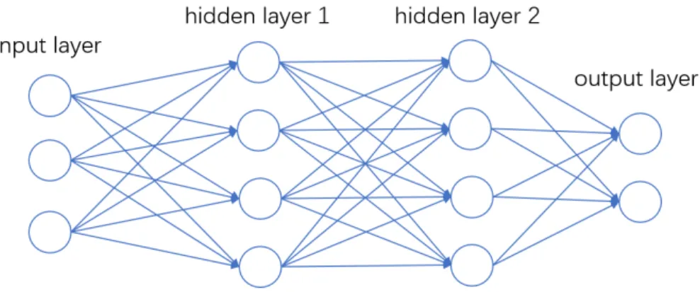
Figure 2.2: Typical structure of feed-forward neural networks (FNN).

There are many structural variants of NNs. Among them, the regular feed-forward neural networks (FNN) are of the simplest kind. The typical structure of FNNs is shown in figure 2.2. As shown in the figure, FNNs have an input layer, multiple hidden layer and an output layer, arranged sequentially. The adjacent

(34)

layers in the network are fully connected and there is no intra-connection within each layer. Note that there is no cyclic connection in the network, and this is why it is called feed-forward neural network.

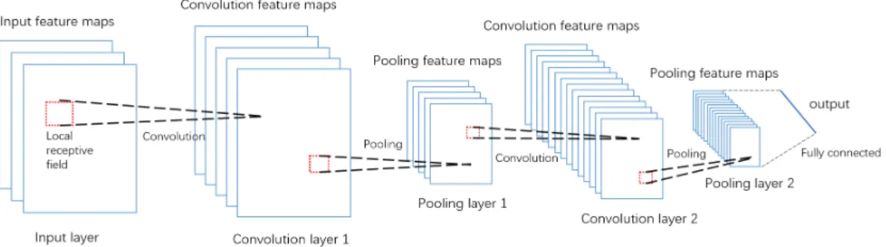
Figure 2.3: Typical structure of convolutional neural networks (CNN).

Another well-known type of neural network variant is the convolutional neural network (CNN) [24], which is specially designed to handle images. As shown in figure 2.3, CNNs typically contain several pairs of convolution layer and pooling (subsampling) layer. Each layer has a number of feature maps of the same size, with each of them representing one kind of feature extracted from different locations of the previous layer’s feature maps. In the convolution layer, CNNs swipe over the input image feature maps and apply convolution operation on small regions of the image called local receptive fields; these convolution operations on each of the small regions share the same convolution weights. This mechanism of convolution on small regions is designed to extract local features of the images. In the pooling

(35)

layer, with the local features detected on the previous convolution layer, CNNs perform pooling operations on small regions to select or combine the local features in the convolution layer. This pooling operation has the purpose of generalizing lower-level features as well as to reduce resolution of the feature maps. These mechanisms together, can help CNNs to handle the local shifts and distortions often seen in images.

Figure 2.4: Typical structure of recurrent neural networks (RNN).

In the FNNs and CNNs, the network output depends only on the current input and no historical information is used. Recurrent neural network (RNN) is a differ-ent type of network architecture that can take into account historical information by its recurrent structure. As shown in figure 2.4, RNN has a cyclic connection that connects the hidden layer back to itself. In this way, not only the current input, but also the previous state of the hidden layer contributes to the current state of the hidden layer; hence the state of hidden layer serves as a memory of the historical information. During training, RNNs usually need to be unfolded

(36)

to allow error information to back-propagate to inputs at every timestamp. This propagation through previous states operation is usually referred to as back-propagation through time (BPTT) [39]. Since error information in RNNs need to back-propagate through a sequence of unfolded previous layers, it is usually much harder to train RNNs than regular FNNs. And moreover, gradients will often grad-ually vanish or explode along a series of multiplications in the back-propagation procedure, which becomes a major difficulty in training RNNs [16].

The Long Short Term Memory network (LSTM) [15] is a kind of RNN that is specially designed to avoid the vanishing gradient problem. LSTM has the chain of repeating modules structure like standard RNNs. But within each module, in-stead of using a single activation function on the input and the previous hidden state, LSTM uses a complicated gating mechanism to control the forgetting and updating of the hidden state and the output. Hence unlike RNN that can only capture the short-term dependencies, LSTM is also capable of capturing long-term dependencies.

2.2.4 Optimization algorithms

In order to guide the learning process towards a better solution, we need to set an evaluation metric for the learning. Such an evaluation metric can be defined

(37)

as a function that maps a parameter setting to a real number. Conventionally in machine learning, this number is designed to represent some ”cost” that needs to be minimized. Hence the defined function is often called the cost function, or also referred to as loss function, error function or objective function. The task of optimization in machine learning is to find the set of model parameters that minimizes the loss function.

There are many optimization algorithms that exist for the training of neural networks. Stochastic gradient descent (SGD) [5] is probably the most famous one. In the original gradient descent algorithm, the learning process iteratively takes steps proportional to the negative of the gradient of the loss function at the current point. Let L(·) denote the loss function and Wt denote the model weights at the

t-th iterative step, a gradient descent updating step can be represented as:

Wt+1 =Wt−γ· ∇L(Wt) (2.2) where γ is a small step size called the learning rate, and ∇L(Wt) denotes the gradient of the loss function. The loss functionL(W), in practice usually comprises a sum of terms, one for each training sample in the dataset:

L(W) = 1 N N X n=1 Ln(W) (2.3)

whereLn(W) is the loss function on then-th data sample with the models weights W. In each iterative update step, the algorithm needs to compute the gradients

(38)

summed over all the data samples, which is a heavy computation for large datasets. In this case, stochastic gradient descent (SGD) approximates the true gradient by the gradient of a randomly picked single data sample (or a mini-batch of data samples in practice):

Wt+1 =Wt−γ · ∇Ln(Wt) (2.4)

In this way, the algorithm avoids the heavy summation computation in each iter-ative update step. And moreover, the randomness introduced in each update step can help the model to move out of some local minima. Although using an inaccu-rate gradient in each update step, it has been proven that SGD can almost surely converge to a local minimum, under some minor assumptions [5]. In practice, we refer an epoch as a complete traversal of the whole dataset. In the start of every epoch, the dataset is randomly divided into a number of mini-batches and one up-date step will be performed on each mini-batch. This implementation is sometimes referred to as mini-batch gradient descent.

Adam [21] is another efficient gradient-based optimization algorithm. It has a more complex mechanism for weight updating that combines with momentum and second moments of the gradients. In thet-th iteration, the algorithm updates

(39)

model weights according to the following formulae: mt+1 =β1·mt+ (1−β1)· ∇L(Wt) (2.5) vt+1=β2·vt+ (1−β2)·(∇L(Wt))2 (2.6) ˆ m= m t+1 1−β1t (2.7) ˆ v = v t+1 1−β2t (2.8) Wt+1 =Wt−γ ·√mˆ ˆ v+ (2.9)

where is a small number used to prevent division by 0, and β1 and β2 are the

forgetting factors for the moving averages of the first and second moments of the gradients. The recommended values for these parameters are: = 1e−8, β1 = 0.9

and β2 = 0.999 as in [21]. We use the these recommended values in our

imple-mentation. Adam is a per-parameter adaptive learning rate method because the gradient of each model weight is individually and automatically adjusted based on the history of the first and second moments of the gradient. However, a learning rate annealing schedule is still necessary for training.

Learning rate is one of the common but very important hyper-parameters in the training of NNs. As shown in equation 2.2, learning rate is a hyper-parameter to control the step of updates. If learning rate is set too large, the learning may not converge. On the other hand, if the learning rate is too small, the learning speed

(40)

will be very slow. Learning rate typically needs to decrease along with the training of NNs. A scheme that specifies how learning rate decreases is call the learning rate annealing schedule. There are many learning rate annealing schedules, ranging from simple schedule like multiplying with a constant factor (<1) to more complicated mechanism like only halving the learning rate when no improvement is observed.

2.2.5 Error back-propagation

Figure 2.5: Illustration of the back-propagation mechanism. The blue arrow denotes the forward direction of information flow, and the red arrows denotes the direction of the error back-propagation.

As we have seen from the above subsection, the training of neural networks often involves the computation of gradients for all the adaptive weights at each update step, which is usually the most computationally expensive part in the training pro-cess. Back-propagation [36] is a well-known algorithm that can compute gradients

(41)

of all adaptive weights simultaneously. It is commonly used as a part of iterative optimization algorithms because of its efficiency in computing gradients. As shown in equation 2.3, loss functions usually comprise of a sum of terms. In this case, it is sufficient for us to first derive the gradients for only one training sample and then generalize to more samples. Consider an arbitrary neuron j, as shown in the figure 2.5. The desired gradient of the loss function with respect to an adaptive weightwij can be expressed, according to the chain rule for partial derivatives, as:

∂Ln(W) ∂wij = ∂Ln(W) ∂aj · ∂aj ∂wij = ∂Ln(W) ∂aj ·zi (2.10)

Letεj denote ∂L_∂an(W_j ), the formula to compute the gradient of weight wij becomes: ∂Ln(W)

∂wij

=εj ·zi (2.11)

Now we turn to the termεj, which can also be decomposed by the chain rule as: εj = ∂Ln(W) ∂aj = ∂Ln(W) ∂zj · ∂zj ∂aj =f0(aj)· X ∀k,∃wjk ∂Ln(W) ∂ak · ∂ak ∂zj =f0(aj)· X ∀k,∃wjk εk·wjk (2.12) We refer the term εj as error. According to the above formula, the error term

can be computed backward using the error terms of the neurons in the next layer. This is why it is called the error propagation algorithm. In general, the back-propagation algorithm uses the following procedure:

(42)

1. Feed the inputs into the neural network, compute allz’s anda’s in the forward phase using formula 2.1;

2. Get the error terms of the output neurons, which can be computed based on the specific loss function used;

3. Back-propagate errors from the output neurons to the other neurons layer by layer, according to formula 2.12;

4. Compute the gradients with respect to the adaptive weights with formula 2.11;

5. Update model weights following formula 2.2;

2.3 Related Works

In this section, we will briefly describe some of the related works that we are going to compare our model performance with. These related works include a LDA based generative model and some neural network based models.

2.3.1 LDA and its based model for text classification

The Latent Dirichlet allocation (LDA) model [4] is a popular generative model for text modeling. It is a three-level hierarchical model in which each document is rep-resented as a random mixture of latent topics, and each latent topic is characterized

(43)

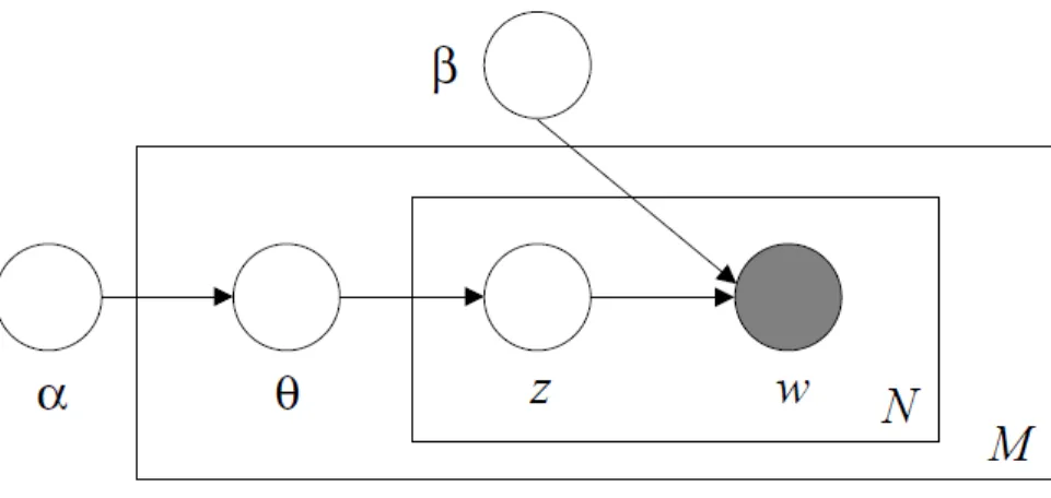
Figure 2.6: Graphical model representation of LDA. The boxes are ”plates” rep-resenting replicates. The outer plate represents documents, while the inner plate represents the repeated choice of topics and words within a document. (This figure is from [4]).

(44)

by a distribution over words. By introducing the level of mixture of latent topics, LDA is able to associate multiple topics with a document. Comparing with many other clustering models that restrict a document to be associated with a single topic, the flexibility of repeatedly selecting and switching topics within a document makes LDA more powerful to model real-world documents. However, like most of the other models, LDA follows the assumption of exchangeability for simplicity, which ignores the order of words in a document.

LDA assumes the following generative process to generate a document:

1. Choose document length N ∼ Poisson (λ), where λ is the average document length in the current setting.

2. Choose topic selecting probabilities θ ∼ Dir (α), where α is a parameter vector of positive reals.

3. For each of the N words wn:

(a) Choose a topic zn ∼Multinomial (θ).

(b) Choose a word wn ∼ Multinomial (β(zn,:)), a multinomial probability

distribution conditioned on the topic zn.

(45)

a Dirichlet distribution: p(θ | α) = Γ( PK i=1αi) QK i=1Γ(αi) K Y i=1 θαi−1 i (2.13)

where α is a K-dimensional parameter vector with components αi > 0, K is the

total number of possible topics, and Γ(·) is the Gamma function. According to the property of Dirichlet distribution,θ takes values in the (K−1)-dimensional simplex so that ∀i, θi ≥ 0 &

PK

i=1θi = 1. Therefore θ is used to represent probabilities of

selecting each topic in a topic selection step during the generation of this document. After defining the θ, the process then repeatedly generates a word until it reaches the document length. In the generation of each word, the process first selects a topic zn from all K topics following the multinomial distribution Multinomial (θ).

Then based on the selected topic zn and β, which is a K×V matrix that stores

the conditional word probabilities for each topic (i.e., βij = p(wj | zi)), the

pro-cess generates a word according to a topic-conditioned multinomial distribution Multinomial (β(zn,:)).

In the paper [14], Hingmire et al. proposed a document classification algorithm called ClassifyLDA that is based on LDA. In the algorithm, they first construct a topic model using LDA on the corpus, then they manually assign a class label to each of the learned topics according to expert knowledge. After that, they aggregate all the topics within each class into a single topic for that class using

(46)

the aggregation property of the Dirichlet distribution. With the aggregated topics associated with the classes, the system then can automatically classify an unlabeled document depending on its ”closeness” to the class topics. Based on this algorithm, they further extend to build a na¨ıve Bayes classifier for text classification and use the well-known Expectation-Maximization (EM) algorithm for optimization.

2.3.2 Neural network based models for text classification

Many of the current best NN-based models for text classification typically use some recurrent structure to handle the variable-length text documents and to capture context information for training.

Figure 2.7: Structure of the recurrent convolutional neural network (RCNN). (This figure is from [22]).

(47)

In [22], Lai et al. proposed a recurrent convolutional neural network (RCNN) that combines a recurrent structure and a max-pooling layer to extract useful fea-tures from variable-length text documents. As shown in figure 2.7, a bi-directional recurrent structure is used to recursively encode context information around each word in the text document. The left and right context vectors are encoded using the following formula:

cl(wi) = f(W(l)cl(wi−1) +Wsle(wi−1))

cr(wi) = f(W(r)cr(wi+1) +Wsre(wi+1))

where cl(wi) and cr(wi) are the left and right context vectors of word wi, e(wi)

denotes the word embedding of word wi and W(l), W(r), Wsl and Wsr are weights

to be learned. The corresponding left-context, center word and the right context vectors are concatenated to generate the context representation xi for each center

word. Then each of the context representations is multiplied with a weight matrix and fed into a tanh activation function to generate a latent semantic vector yi.

After that, a max-pooling layer is used to select useful features element-wise from the latent semantic vectors. Based on the selected features, a fully connected layer is used to generate outputs. They called the recurrent structure the convolutional layer though there is no convolution operation performed.

(48)

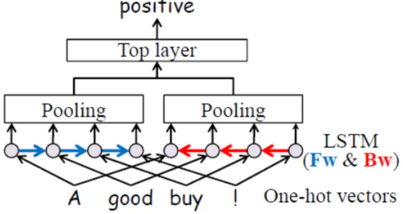
Figure 2.8: Structure of the one-hot bidirectional LSTM with pooling model (oh-2LSTMp). (This figure is from [20]).

backward context of a text sequence. In their model, as shown in figure 2.8, they removed the embedding layer and directly built the LSTMs on one-hot vectors. The pooling layers then pool over all the intermediate outputs of LSTMs. After pooling, a fully connected layer is then applied to generate outputs.

Instead of learning model directly from labeled data, Dai et al. [8] used a semi-supervised approach to first unsemi-supervisedly train a LSTM model for the language modeling task, which is a task to predict the next word in natural language text se-quence based on the previous words, and then they fine-tune the pre-trained LSTM on the text classification datasets. In this way, they can make use of the enormous amount of unlabeled data to help the model start from a better initialization point.

(49)

3 Context-FOFE Encoding Scheme

Most of the machine learning algorithms need to have fixed-size inputs. How-ever, natural language sentences are usually of variable length. Some models try to handle this problem by truncating the long sentences and padding the short sentences [17, 44], which is unnatural and suffers from losing information. Bag of words (BoW) representation is a simple and commonly used method that can be used to convert variable-length text into a fixed-size vector, nevertheless, this representation discards the most important word ordering information in the text, thus limiting the system performance.

Moreover, one of our goals in this work is to design a representation method for variable-length text documents that can encode their informative contexts. The context patterns, according to our assumption stated in section 1.1, are very good features for text classification. However, these context patterns are hidden within text documents and need to be discovered by classification models through a learn-ing process. In this sense, our desired representation is better to be simple but

(50)

informative.

To meet these demands, we propose a recursive encoding scheme that can con-vert variable-length text into fixed-size representation while retaining the word ordering information. Furthermore, the encoded representation is unique and re-versible for every piece of text. We call this encoding scheme Context-FOFE, for it is based on the Fixed-size Ordinally Forgetting Encoding (FOFE) scheme [41, 42], and focuses on keeping all the context (word ordering) information.

In the following sections, we will first introduce the FOFE encoding scheme, which forms the basis of our context encoding scheme; then we will describe how our context-FOFE encoding scheme encodes context information; lastly we will present an efficient implementation of our encoding scheme.

3.1 The FOFE Encoding Scheme

FOFE is a simple recursive encoding scheme that can almost uniquely encode any sequence of words (or discrete symbols), with their ordering information, into a fixed-size representation. FOFE memorizes the word order in a text sequence using a simple ordinally-forgetting mechanism that relates weights of the words with their positions in the sequence. In the papers [41, 42], Zhang et al. have shown that FOFE has the equivalent ability as RNNs to encode historical information.

(51)

And moreover, since the encoding is based on a simple recursive formula, there is no parameter needs to be learned.

FOFE’s ordinally-forgetting mechanism works as follows. Given a sequence of words S ={w1, w2, . . . , wT}, each word wt is first represented as a 1-of-V one-hot

vectoret, wheret(1≤t≤T) denotes the sequential reading step andV denotes the

vocabulary size. FOFE then encodes the sequence word by word from the beginning to the end of the sequence based on the following simple recursive formula (with

Z0 =0):

Zt=α·Zt−1 +et (3.1)

WhereZtdenotes the FOFE code for the partial sequence up to wordwtandα(0< α < 1) is a constant forgetting factor that controls the contribution of historical information to the current encoding. The constantα is called the forgetting factor because the weights of the previous words are gradually reduced byαas the reading moves forward. By using such an ordinally-forgetting mechanism, FOFE efficiently relates the weights of words with their positions in the sequence. According to the weights in the encoded representation, it is also possible to revert the FOFE code back to the original word sequence.

Figure 3.1 shows examples of using FOFE to encode word sequence. In the figure, the table to the left contains the vocabulary list and the corresponding

(52)

one-Figure 3.1: Illustration of the FOFE encoding scheme.

hot vectors of each word. The one-hot vectors are of vocabulary size, with each word corresponding to a different position in the vector. The table to the right shows the FOFE code for each intermediate partial sequence. Each time a new word is read in, the FOFE code is first multiplied with the forgetting factor α, and then added with the corresponding one-hot vector of the read-in word. Following this procedure, the sentence ”to be or not to be”, with a vocabulary list as{”to”, ”be”, ”or”, ”not”}, is represented in FOFE as ”[α+α5,1 +α4, α3, α2]”. Comparing with its bag-of-words representation ”[2,2,1,1]”, which we have shown in section 1.1, obviously the FOFE code can better represent the sentence as its weights reflect the word orders in the sentence.

The FOFE code for any sequence of words is almost unique, given the vo-cabulary is sufficiently large to include all possible words in the text sequences.

(53)

Here the unique encoding means a one-one mapping between text sequences and FOFE codes. That is, for any two different text sequences, they will have different FOFE codes; for any sequence of words, given its FOFE code, the vocabulary list and forgetting factor used, it should be able to unambiguously recover the original sequence. The uniqueness property of FOFE encoding has been proven both the-oretically and experimentally. Thethe-oretically, when 0 < α ≤ 0.5, according to the formula of the sum of geometric series, we have:

t X i=1 αi = α(1−α t₎ 1−α <tlim→∞ α(1−αt₎ 1−α = α 1−α ≤1

Hence at any intermediate time step, there can be only one weight that is greater than or equal to 1, which corresponds to the word that just read in. Based on this fact, it is easy to decode the FOFE code to the original word sequence; just reverse the encoding procedure. Experimentally, the authors have tested all the possible sequences up to 20 words for number of collisions. A collision is defined as the event in which the maximum element-wise difference between two FOFE codes is less than a set small error. In the experiments, the authors found that the number of collisions is extremely small, thousands of collisions out of 1020 _{tested sequences,}

even with no restriction on the possible word sequences. In real-world situation, with the syntactic and semantic restrictions of natural language, the number of collisions would be much less. This phenomenon can be heuristically explained by

(54)

the sparsity of natural language. Here the sparsity of natural language refers to the facts that a piece of natural language text usually only uses a small portion of the vocabulary, and normally there is very few sentences in a text document having exactly the same sequence of words. In this case, we can conclude that the FOFE encoding scheme can encode any sequence of words into almost unique representation, given a sufficiently large vocabulary.

3.2 The Context-FOFE Encoding Scheme

As introduced in section 3.1, FOFE can almost uniquely encode text of variable length into a fixed-size vector representation while keeping its word ordering in-formation. Having all these exciting properties, we may think of using FOFE to encode text documents. Since FOFE already keeps the word ordering information of the text document, the context information should also have been encoded. This sounds reasonable in theory. However, in practice the FOFE code can only remem-ber recent history because of the fact that weight αt becomes insignificant as the power term t gets larger. Moreover, FOFE puts more weight on the later words of a text sequence because FOFE’s encoding process is a recursive process in which weights of the previous words are decreased each time a new word is read in. This biased weight distribution will let the learning model unnecessarily focus on the

(55)

later part of the text document.

(a) (b)

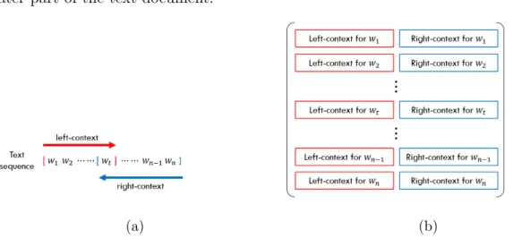
Figure 3.2: Context-FOFE encoding scheme. (a) Context around word wt. Words

are represented as one-hot vectors. (b) Context matrix. The context vectors are of the same size.

To overcome this difficulty when encoding long text sequences like documents, and to fully encode context information with unbiased focus, we propose a variant of the FOFE encoding scheme, namely, the Context-FOFE encoding scheme. This scheme encodes the context information of a text document into a matrix. As shown in figure 3.2a, the context around wordwt is divided into a left-context and

a right-context, where the left-context denotes the forward word sequence from

w1 to wt, and the right-context denotes the backward word sequence from wn to wt. We use FOFE to encode the left-context and the right-context, respectively.

(56)

generate a row vector that represents the context around the center word. For each word in a text document, we can generate a row vector. And by concatenating these row vectors vertically according to the word order, we can form a matrix of size N ×2V, whereN is the length of the text document and V is the vocabulary size, as shown in figure 3.2b. We call this matrix as context matrix and use it to represent the corresponding text document.

As a simple encoding scheme that can uniquely encode context information of text documents into a matrix containing fixed-size vectors, our context-FOFE keeps all the merits of the FOFE encoding scheme. Firstly, our context-FOFE en-coding scheme enhances FOFE to have complete uniqueness and reversibility on the encoded representation, under the same condition of having a sufficiently large vocabulary. Since our matrix representation of text document consist of FOFE codes for all the word positions, that is, all the partial word sequences, it is very easy to revert back to the original text sequence. And because for any encoded representation, we can unambiguously recover the original text sequence, we say our method can encode any text document into completely unique representation. Secondly, our encoded representations of text documents are generally applicable to many machine learning models that require fixed-size inputs. Our matrix repre-sentation of text document comprises fixed-size vectors; each one of these fixed-size

(57)

vectors can be fed as input to many machine learning models. Thirdly, the same as FOFE, our encoding process is a simple recursive process that is only controlled by a single hyper-parameter called forgetting factor. This makes our method an efficient and fast encoding method.

Furthermore, our context-FOFE encoding scheme has the following extra bene-fits. Firstly, our method solves the biased focus problem arose when encoding long text sequences with FOFE. Instead of sampling context patterns once only with a focus on the latter words, we sample context patterns at every word position and hence every position in the document is focused on. Secondly, The context patterns sampled at every word position can provide slightly different views of a document, which can potentially make the learning of context patterns easier. Finally, by sam-pling the slightly different views of a document at each word position, our method effectively augments the existing training data to provide more data for training.

3.3 Efficient Implementation of Context-FOFE

Although our context-FOFE encoding scheme is based on a recursive encoding formula, in implementation we don’t have to follow the recursive process iteratively to encode text documents. Note that our context-FOFE encoding only has one single parameter, the forgetting factorα; and according to the ordinally-forgetting

(58)

mechanism, weights of words are gradually reduced by multiplying withα. We can know that the partial weight of a word resulting from its appearance t positions before is αt. Based on this fact, we can first construct a weight matrix containing positional weights for all partial sequences, as:

                1 α 1 α2 _α ₁ .. . ... ... . .. αL−1 αL−2 αL−3 · · · 1                 (3.2)

where L denotes length of the text document. Note that this is only a weight matrix and does not involve any particular word sequence. Hence this matrix can be generally constructed according to the length of the text sequence. Then to encode a text sequence, we can just multiple this weight matrix with the matrix of

(59)

one-hot vectors of the text sequence: left context=                 1 α 1 α2 _α ₁ .. . ... ... . .. αL−1 αL−2 αL−3 · · · 1                

×[rows of 1-hot vectors] (3.3)

right context=                 1 α 1 α2 _α ₁ .. . ... ... . .. αL−1 αL−2 αL−3 · · · 1                 T

×[rows of 1-hot vectors] (3.4)

(3.5)

where the one-hot vectors should be in the same order as the corresponding words in the text sequence.

Noticing that weights αt _{are gradually reduced and become insignificant when} t gets larger, we can obtain even better efficiency both on speed and memory by removing insignificant weights. To do this, we can set a threshold to prune all

(60)

weights less than the threshold in the weight matrix, as:             1 0 0 0 α 1 0 0 α2 _α ₁ ₀ α3 _α2 _α ₁             =⇒ pruned             1 0 0 0 α 1 0 0 0 α 1 0 0 0 α 1             (3.6)

assumingα2 _{is below the threshold. Clearly, this pruning operation is equivalent to}

setting a context encoding window. For a commonly used forgetting factorα = 0.7 and a threshold 0.001, the effective context window size is 20 including the center word, for either the left context or the right context.

(61)

4 Context-FOFE Based FNNs for Text

Classification

In chapter 3 we presented our novel context-FOFE encoding scheme to convert text documents of variable length into fixed-size representations that as well keep all the context information. Moreover, our context-FOFE representation has extra benefits like: uniqueness, reversibility and effectively providing more training data. In this chapter, we are going to design NN models to test our feature representation method on the text classification task. We decide to use the regular feed-forward neural network (FNN) rather than the recurrent neural network (RNN) because each row of the context-FOFE encoded representation has already captured the surrounding context information, hence no need for the internal memory of the previous context and the sequential reading of the text. Moreover, as we already know, FNNs have much simpler structure than RNNs and hence are much easier and faster to train.

(62)

Our context-FOFE encoding scheme encodes text document into a matrix that contains many fixed-size vectors, with each vector representing the context around a word. With these many fixed-size vectors in every document, naturally we can have two ways to train the NN model. The first way is to treat each vector representation in a document as an individual training instance and train on them independently; the second way is to treat the whole matrix representation as an individual training instance, and feed in the vector representations of all the word positions within the document as a whole for training. The NNs for the two ways of training share similar structure and the difference only occurs on aggregating position-wise hidden representations to a vector representation of the whole document.

4.1 Position-wise Trained Model

According to the context-FOFE encoding scheme, each word position generates a tuple of left-context FOFE code and right-context FOFE code. In position-wise training, each tuple of the context-FOFE codes is treated as a training instance. And the tuples are shuffled over the whole dataset. In this way, we mix up the relationships between adjacent tuples and view each tuple of the context-FOFE codes as an individual text sequence. This effectively provides more text sequences for training, even though many of them are similar.

(63)

Although the context-FOFE code has already kept all the context informa-tion necessary for training, the representainforma-tion itself is sparse and high-dimensional. Moreover, there is no semantic relation between words. In this case, it is necessary to multiply the FOFE codes with a projection matrix to perform the dimension re-duction. In addition, the projection matrix can be initialized by a word embedding matrix to further relate the words in the semantic space.

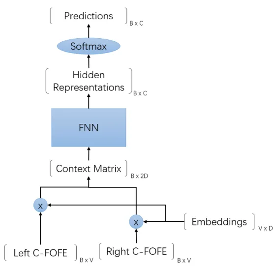
As shown in figure 4.1, the left-context FOFE codes and the right-context FOFE codes of a mini-batch of the training instances are first projected onto the semantic space by multiplying with a shared word embedding matrix. The shared word embedding matrix can be fine-tuned during training to better adapt to the specific dataset, and hence it can be viewed as part of the model weights. The left and right projected contexts are then concatenated horizontally, with the corresponding rows aligned, to form a B ×2D context matrix, which are the features of the training instances in the semantic space. After that the context matrix is fed into the regular FNN. Each layer of the FNN serves as a feature abstractor that abstracts the features to a higher level. We call the highly abstracted feature representations in the last hidden layer the hidden representations of the sample instances. On top of these highly abstracted representations of the training instances, we then use a

(64)

Figure 4.1: Structure of position-wise trained FNN.B denotes the mini-batch size;

V denotes the vocabulary size; D denotes the word embedding dimension and C

(65)

softmax layer to predict the labels of the training instances: pi =softmax(h) = ehi PC k ehk fori= 1,· · · , C (4.1)

wherehi denotes the i-th element of the hidden representation, andpi denotes the i-th element of the output vector. The softmax function normalizes the outputs to have a sum equal to 1, hence the outputs can be viewed as the predicted likelihood scores for each of the categories.

Note that we have labels for the training text documents but not for every word position. In this case, to obtain training labels for all training instances, we simply assign the document label to all the word positions within the document. This is reasonable because we assume context patterns are distinct in different text categories but similar in the same text category. Therefore training instances within a document probably have similar category label as the document. According to this labeling mechanism, the loss function for training is defined as the cross-entropy function over all the training instances:

L=− 1 N N X i=1 Tilog(Pi) (4.2)

whereN is the total number of word positions in the whole dataset,Ti is the label

vector for the i-th training instance and Pi is the softmax output vector for the i-th training instance.

(66)

4.1.1 Voting strategy

Our position-wise FNN model is trained to predict the word positional labels. How-ever, in testing we need to predict the document label. In order to obtain the document label, we need a mechanism to aggregate the information from word po-sitions within the document. We call such a mechanism a voting strategy, for it is a mechanism for every word position to contribute their scores against each category to the final score.

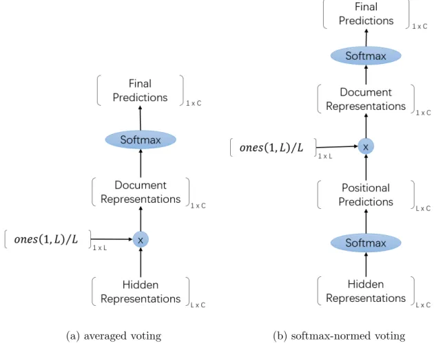
Since we can feed all the word positions of a document into the trained model to produce the corresponding hidden representations, a very natural way to aggre-gate the position-wise information is to take the element-wise average of the hidden representations, and use the averaged hidden representation to represent the doc-ument, as shown in figure 4.2a. With the document hidden representation vector, it is then easy to generate the category predictions; just feed it into the softmax layer. We call this simple mechanism the averaged voting strategy.

Remember that the outputs of the softmax layer for each word position can be viewed as the predicted likelihood scores for each of the categories. With the likelihood scores from all the word positions, we can compute the document level likelihood scores for each of the categories, as an average of the position-wise likeli-hood scores. we call this mechanism the softmax-normed voting strategy. As shown

(67)

(a) averaged voting (b) softmax-normed voting

Figure 4.2: Voting strategies for context-FOFE based FNNs. L denotes the docu-ment length.

(68)

in figure 4.2b, there are two softmax layers. The first one is to get the position-wise predicted likelihood scores, and the second one is to generate the final document level prediction scores. Comparing with the averaged voting, the softmax-normed voting can balance the contributions of word positions to the document level repre-sentation by normalizing the weights across categories on each position. But having two softmax layers stacked together makes it more complicated than the averaged voting.

4.2 Document-wise Trained Model

In the position-wise training, the model is trained with shuffled position-wise train-ing instances but tested document-wise. This may lead to a mismatch between the loss function and the performance goal. To avoid this mismatch and gain potential performance improvement, we can train the model document-wise.

In document-wise training, each context-FOFE matrix as a whole is treated as a training instance. Hence the training data are shuffled on the document level instead of the word position level. Furthermore, as part of a whole, the context vectors of all the word positions within the document are needed to be fed into the network at the same time. Also, the back-propagated gradients of this training instance need to be averaged over all word positions.