Meta-analysis with
application to estimating
combined estimators of effect
sizes in biomedical research.
Mhlengi Corrigan Mgaga November, 2018
Meta-analysis with application to estimating
combined estimators of effect sizes in
biomedical research.
byMhlengi Corrigan Mgaga
A thesis submitted to the University of KwaZulu-Natal
in fulfilment of the requirements for the degree of
MASTER OF SCIENCE in
STATISTICS
Thesis Supervisor: Prof Henry Mwambi Thesis Co-supervisor: Prof Ding-Geng Chen
UNIVERSITY OF KWAZULU-NATAL
SCHOOL OFMATHEMATICS, STATISTICS ANDCOMPUTERSCIENCE
Declaration - Plagiarism
I, Mhlengi Corrigan Mgaga, declare that
1. The research reported in this thesis, except where otherwise indicated, is my original research.
2. This thesis has not been submitted for any degree or examination at any other university.
3. This thesis does not contain other persons’ data, pictures, graphs or other in-formation, unless specifically acknowlegded as being sourced from other per-sons.
4. This thesis does not contain other persons’ writing, unless specifically acknowl-edged as being sourced from other researchers. Where other written sources have been quoted, then
(a) their words have been re-written but the general information attributed to them has been referenced, or
(b) where their exact words have been used, then their writing has been placed in italics and referenced.
5. This thesis does not contain text, graphics or tables copied and pasted from the internet, unless specifically acknowledged, and the source being detailed in the thesis and in the reference sections.
Mhlengi Corrigan Mgaga (Student) Date
Prof Henry Mwambi (Supervisor) Date
Disclaimer
This document describes work undertaken as a Masters programme of study at the University of KwaZulu-Natal (UKZN). All views and opinions expressed therein remain the sole responsibility of the author, and do not necessarily represent those of the institution.
Abstract
Meta-analysis is a statistical analysis that combines results from different indepen-dent studies. In meta-analysis a number of statistical methods are currently used for combining effect sizes of different studies. The simplest of these methods is based on a fixed-effects model, which assumes that all studies in the meta-analysis share a common true effect size and that the effect sizes in our meta-analysis differ only because of sampling error. Another statistical method that is used in meta-analysis, is the random-effects model, which assumes sampling variation due to fixed-effects model assumptions and random variation because the effect sizes themselves are sampled from a population of effect sizes. These models are compared to determine which model is appropriate and under what circumstances is the model appropriate. We illustrate these models by applying each model to a collection of 3 studies exam-ining the effectiveness of new drug versus placebo to treat patients with duodenal ulcers and meta-analysis of 9 studies of the use of diuretics during pregnancy to pre-vent the development of pre-eclampsia. Results indicated that the choice between the two model depends on the question of which model fits the distribution of effect sizes better and takes account of the relevant source(s) of error. We further study the meta-analysis of longitudinal studies where effect sizes are reported at multiple time points. Univariate meta-analysis is a statistical approach which may be used to study effect sizes reported at multiple time point. The problem with this approach is that it ignores correlation between the effect sizes, which might increase the stan-dard error of the point estimates. We used the linear mixed-effects model, which borrows ideas from multivariate meta-analysis. One of the advantages of the lin-ear mixed-effects model is that it accounts for correlation between effect sizes both within and between studies. The independence model where separate univariate meta-analysis is done at each of the time points was compared against models where correlation was accounted for different alternatives; including random study effects, correlated random time effects and/or correlated within-study errors, or unstruc-tured covariance structures. We implemented these methods through an example of meta-analysis of 16 randomized clinical trials of radiotherapy and chemotherapy versus radiotherapy alone for the post-operative treatment of patients with
malig-nant gliomas, where in each trial, survival is evaluated at 6, 12, 18 and 24 months post randomization. The results revealed that models that accounted for correlations had better fit.
Keywords: meta-analysis, fixed-effects model, random-effects model, heterogeneity, publication bias, linear mixed-effects model.
Acknowledgements
Firstly, I would like to thank my supervisor Prof. Henry Mwambi for his presence, guidance and invaluable advice throughout this research. I again thank him for reading and correcting my errors in this research. Secondly I would like to thank my co-supervisor Prof. Ding-Geng Chen for willing to work with me. Much thanks for his guidance, help and responses whenever I consulted. Many thank to him for correcting my research.
I am grateful for the scholarship awarded to me by DELTAS Africa, without which I would have been unable to support myself during the year of my research. The DELTAS Africa Initiative is an independent funding scheme of the African Academy of Sciences (AAS)’s Alliance for Accelerating Excellence in Science in Africa (AESA) and supported by the New Partnership for Africa’s Development Planning and Co-ordinating Agency (NEPAD Agency) with funding from the Wellcome Trust [grant 107754/Z/15/Z-DELTAS Africa Sub-Saharan Africa Consortium for Advanced Bio-statistics (SSACAB) programme] and the UK government. The views expressed in this publication are those of the author(s) and not necessarily those of AAS, NEPAD Agency, Wellcome Trust or the UK government.
Finally, I wish to express my appreciation to my family and friends, for their support and encouragement. I may not count every one but I am grateful to everyone who helped me.
Contents
Page
List of Figures xi
List of Tables xiii
Chapter 1: Introduction 1
1.0.1 Effect size . . . 2
1.0.2 Objectives of the study . . . 5
1.0.3 Outline of the study . . . 5
Chapter 2: Overview of basic statistical concepts and approaches in meta-analysis 6 2.1 Preliminary concepts . . . 6
2.2 Effect sizes based on binary data (2×2 tables) . . . 6
2.2.1 Risk difference . . . 7
2.2.2 Relative risk . . . 8
2.2.3 Odds ratio . . . 10
2.3 Fixed-effects model . . . 13
2.3.1 Model description . . . 13
2.4 Multivariate Test of Hypotheses . . . 14
2.4.1 Multivariate Null Hypothesis . . . 14
2.4.2 Tests for Homogeneity . . . 15
2.4.3 Contrast Test for Homogeneity . . . 15
2.5 Heterogeneity . . . 17
2.5.1 Causes of heterogeneity in meta-analysis . . . 18
2.6 Random-effects model . . . 19
2.6.1 Model description . . . 19
2.7 Choice between fixed-effects and random-effects models . . . 23
2.8 The likelihood method . . . 24
CONTENTS
2.9 Publication bias . . . 27
2.10 Forest Plot . . . 31
Chapter 3: Meta-analysis for longitudinal studies 33 3.1 Introduction . . . 33
3.2 Theory of the linear mixed-effects model for meta-analysis . . . 35
3.2.1 Model description . . . 36
3.2.2 Estimating fixed-effects for V known . . . 41
3.2.3 Predicting random-effects for V know . . . 44
3.2.4 Predicting random-effects for V unknown . . . 46
3.2.5 Maximum likelihood estimation . . . 46
3.2.6 Estimating fixed-effects for V unknown . . . 47
3.2.7 Restricted maximum likelihood estimation . . . 50
3.3 Inference . . . 51
3.3.1 The likelihood ratio test(LR) . . . 51
3.3.2 Wald test . . . 52
3.3.3 Estimating the random-effects . . . 53
3.4 Model selection . . . 55
3.4.1 Akaike information criteria . . . 55
3.4.2 Schwarz criterion . . . 56
3.5 Checking model assumption(diagnostics) . . . 56
3.5.1 Residual diagnostics . . . 57
3.5.2 Conditional and marginal residuals . . . 57
3.5.3 Standardized and studentized residuals . . . 57
3.5.4 Influence diagnostics . . . 58
3.5.5 Overall influence . . . 58
3.5.6 Change in parameter estimates . . . 59
3.5.7 Change in precision of estimates . . . 60
3.5.8 Effect on fitted and predicted values . . . 61
3.5.9 Types of covariance structures . . . 61
3.6 Modelling covariance structures . . . 62
3.6.1 Model 1- Independent random time effects model . . . 63
3.6.2 Model 2- Random study effects model . . . 63
3.6.3 Model 3- Correlated random time effects model . . . 64
3.6.4 Model 4- Correlated within-study effect sizes model . . . 64
3.6.5 Model 5- Correlated within-study effect sizes and correlated ran-dom time effects . . . 65
CONTENTS
3.6.6 Model 6-Correlated random time effects(unstructured) and
corre-lated within-study effect sizes . . . 65
Chapter 4: Application and results 66 4.1 Examples of a univariate meta-analysis . . . 66
4.1.1 Meta-analysis of clinical trial in duodenal ulcers . . . 66
4.1.2 Risk difference . . . 67
4.1.3 Relative risk . . . 70
4.1.4 Odds ratio . . . 73
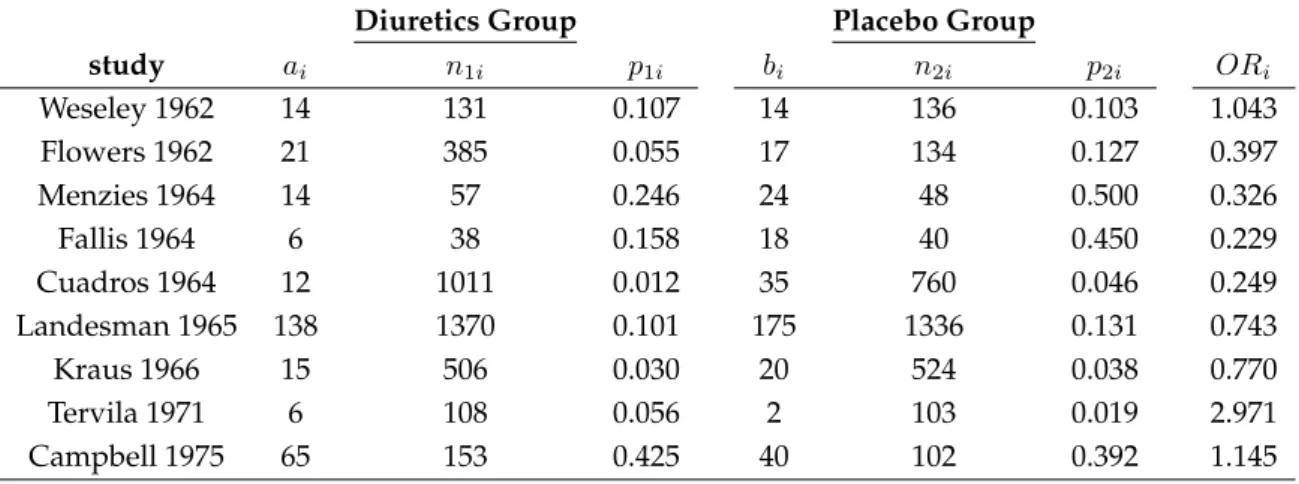
4.1.5 Meta-analysis of effects of diuretics on pre-eclampsia . . . 77
4.1.6 Risk Difference . . . 78
4.1.7 Relative Risk . . . 83
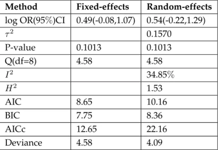
4.1.8 Odds Ratio . . . 89
4.2 Application of the mixed-effects model for meta-analysis . . . 94
4.2.1 Results for the separate univariate random effects meta-analysis . . . 96
4.2.2 Results for the linear mixed-effects model for meta-analysis . . . .105
Chapter 5: Discussion and Conclusion 108
References 118
List of Figures
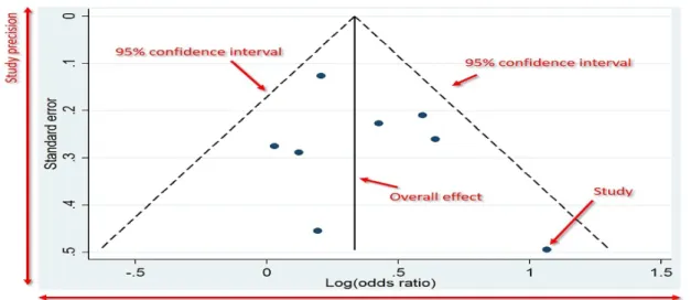
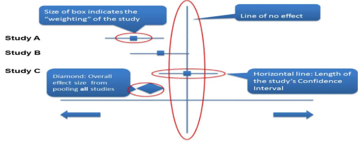
Figure 2.1 Example of the funnel plot. Source:https://toptipbio.com/funnel-plot/funnel-plot-annotated/ . . . 30 Figure 2.2 Example of the forest plot.
Source:https://guides.lib.monash.edu/systematic-review/synthesis/quantitativedata . . . 32 Figure 4.1 Forest plot showing the results of three studies examining the effectiveness
of new drug versus placebo. The figure shows the risk difference of effectiveness of new drug for treatment of duodenal ulcers versus the placebo group with corre-sponding confidence intervals in the individual studies and based on fixed-effects and random-effects models. . . 68 Figure 4.2 Funnel plot shows the risk difference of three studies examining the
effec-tiveness of new drug versus placebo to treat patients with duodenal ulcers. The points corresponds to the treatment effects from individual trials and the diagonal or curved lines show the expected95%confidence intervals around the summary estimate based on fixed-effects and random-effects models. . . 68 Figure 4.3 Plot of the externally standardized residuals, DFFITS values, Cook’s
dis-tance, covariance ratios, estimates ofτ2 and test for residual heterogeneity when each study is removed in turn, hat values, and weights for the 3 studies examining the effectiveness of the new drug versus placebo. . . 69 Figure 4.4 Forest plot showing the results of three studies examining the effectiveness
of new drug versus placebo. The figure shows the log relative risk of effectiveness of new drug for treatment of duodenal ulcers versus the placebo group with corre-sponding confidence intervals in the individual studies and based on fixed-effects and random-effects models. . . 71
LIST OF FIGURES
Figure 4.5 Funnel plot shows the log relative risk of three studies examining the effec-tiveness of new drug versus placebo to treat patients with duodenal ulcers. The points corresponds to the treatment effects from individual trials and the diagonal or curved lines show the expected95%confidence intervals around the summary estimate based on fixed-effects and random-effects models. . . 72 Figure 4.6 Plot of the externally standardized residuals, DFFITS values, Cook’s
dis-tance, covariance ratios, estimates ofτ2 and test for residual heterogeneity when
each study is removed in turn, hat values, and weights for the 3 studies examining the effectiveness of the new drug versus placebo. . . 72 Figure 4.7 Forest plot showing the results of three studies examining the effectiveness
of new drug versus placebo. The figure shows the log odds ratio of effectiveness of the new drug for treatment of duodenal ulcers versus the placebo group with corresponding confidence intervals in the individual studies and based on fixed-effects and random-fixed-effects models. . . 75 Figure 4.8 Funnel plot shows the log odds ratio of three studies examining the
effec-tiveness of new drug versus placebo to treat patients with duodenal ulcers. The points corresponds to the treatment effects from individual trials and the diagonal or curved lines show the expected95%confidence intervals around the summary estimate based on fixed-effects and random-effects models. . . 75 Figure 4.9 Plot of the externally standardized residuals, DFFITS values, Cook’s
dis-tance, covariance ratios, estimates ofτ2 and test for residual heterogeneity when each study is removed in turn, hat values, and weights for the 3 studies examining the effectiveness of the new drug versus placebo. . . 76 Figure 4.10 Forest plot showing the results of nine studies examining the use of
di-uretics during pregnancy to prevent the development of pre-eclampsia. The fig-ure shows the risk difference of pre-eclampsia among those treated with difig-uretics versus the placebo group with corresponding confidence intervals in the individ-ual studies and based on fixed-effects and random-effects models. . . 80
LIST OF FIGURES
Figure 4.11 Funnel plot shows the risk difference of nine studies examining the use of diuretics during pregnancy to prevent the development of pre-eclampsia. The points corresponds to the treatment effects from individual trials and the diagonal or curved lines show the expected95%confidence intervals around the summary estimate and based on fixed-effects and random-effects models. . . 80 Figure 4.12 Plot of the externally standardized residuals, DFFITS values, Cook’s
dis-tance, covariance ratios, estimates ofτ2 and test for residual heterogeneity when
each study is removed in turn, hat values, and weights for the 9 studies examining the use of diuretics during pregnancy to prevent the development of pre-eclampsia. 81 Figure 4.13 Forest plot showing the results of nine studies examining the use of
diuret-ics during pregnancy to prevent the development of pre-eclampsia. The figure shows the log relative risk of pre-eclampsia among those treated with diuretics versus the placebo group with corresponding confidence intervals in the individ-ual studies and based on fixed-effects and random-effects models. . . 85 Figure 4.14 Funnel plot shows the log relative risk of nine studies examining the use
of diuretics during pregnancy to prevent the development of pre-eclampsia. The points corresponds to the treatment effects from individual trials and the diagonal or curved lines show the expected95%confidence intervals around the summary estimate and based on fixed-effects and random-effects models. . . 85 Figure 4.15 Plot of the externally standardized residuals, DFFITS values, Cook’s
dis-tance, covariance ratios, estimates ofτ2 and test for residual heterogeneity when each study is removed in turn, hat values, and weights for the 9 studies examining the use of diuretics during pregnancy to prevent the development of pre-eclampsia. 86 Figure 4.16 Forest plot showing the results of nine studies examining the use of
diuret-ics during pregnancy to prevent the development of pre-eclampsia. The figure shows the log odds ratio of pre-eclampsia among those treated with diuretics ver-sus the placebo group with corresponding confidence intervals in the individual studies and based on fixed-effects and random-effects models. . . 91
LIST OF FIGURES
Figure 4.17 Funnel plot shows the log odds ratio of nine studies examining the use of diuretics during pregnancy to prevent the development of pre-eclampsia. The points corresponds to the treatment effects from individual trials and the diagonal or curved lines show the expected95%confidence intervals around the summary estimate and based on fixed-effects and random-effects models. . . 91 Figure 4.18 Plot of the externally standardized residuals, DFFITS values, Cook’s
dis-tance, covariance ratios, estimates ofτ2 and test for residual heterogeneity when
each study is removed in turn, hat values, and weights for the 9 studies examining the use of diuretics during pregnancy to prevent the development of pre-eclampsia. 92 Figure 4.19 forest plots for month 6, 12, 18 and 24 of the post-operative treatment with
either radiotherapy plus chemotherapy or radiotherapy alone in patients with malignant gliomas from 16 studies. . . 99 Figure 4.20 Funnel plot for month 6, 12, 18 and 24 of the post-operative treatment with
either radiotherapy plus chemotherapy or radiotherapy alone in patients with malignant gliomas from 16 studies. . . 100 Figure 4.21 Plot of the externally standardized residuals, DFFITS values, Cook’s
dis-tance, covariance ratios, estimates ofτ2 and test for residual heterogeneity when each study is removed in turn, hat values, and weights for 16 studies, for month 6 of the post-operative treatment with either radiotherapy plus chemotherapy or radiotherapy alone in patients with malignant gliomas. . . 101 Figure 4.22 Plot of the externally standardized residuals, DFFITS values, Cook’s
dis-tance, covariance ratios, estimates ofτ2 and test for residual heterogeneity when each study is removed in turn, hat values, and weights for 16 studies, for month 12 of the post-operative treatment with either radiotherapy plus chemotherapy or radiotherapy alone in patients with malignant gliomas. . . 101 Figure 4.23 Plot of the externally standardized residuals, DFFITS values, Cook’s
dis-tance, covariance ratios, estimates ofτ2 and test for residual heterogeneity when each study is removed in turn, hat values, and weights for 16 studies, for month 18 of the post-operative treatment with either radiotherapy plus chemotherapy or radiotherapy alone in patients with malignant gliomas. . . 102
LIST OF FIGURES
Figure 4.24 Plot of the externally standardized residuals, DFFITS values, Cook’s dis-tance, covariance ratios, estimates ofτ2 and test for residual heterogeneity when each study is removed in turn, hat values, and weights for 16 studies, for month 24 of the post-operative treatment with either radiotherapy plus chemotherapy or radiotherapy alone in patients with malignant gliomas. . . 102
List of Tables
Table 2.1 A table of follow up randomisation clinical trial . . . 7
Table 4.1 Clinical Trial in Duodenal ulcers. . . 66
Table 4.2 Fixed-effects computations on risk difference. . . 67
Table 4.3 Random-effects computations on risk difference. . . 67
Table 4.4 Results of randomised controlled trials of effect of duodenal ulcers from two methods of meta-analysis. . . 67
Table 4.5 Results of the influence diagnostics for the clinical trial in duodenal ulcers using risk difference as the measure of association. . . 67
Table 4.6 Fixed-effects computations on log relative risk. . . 70
Table 4.7 Random-effects computations on log relative risk. . . 70
Table 4.8 Results of randomised controlled trials of effect of duodenal ulcers from two methods of meta-analysis. . . 70
Table 4.9 Results of the influence diagnostics for the clinical trial in duodenal ulcers using log relative risk as the measure of association. . . 71
Table 4.10 Fixed-effects computations on log odds ratio. . . 73
Table 4.11 Random-effects computations on log odds ratio. . . 74
Table 4.12 Results of randomised controlled trials of effect of duodenal ulcers from two methods of meta-analysis. . . 74
Table 4.13 Results of the influence diagnostics for the clinical trial in duodenal ulcers using log odds ratio as the measure of association. . . 74
Table 4.14 Meta-analysis of nine trials of effects of diuretics on pre-eclampsia. . . 77
Table 4.15 Fixed-effects computations on risk difference. . . 78
Table 4.16 Random-effects computations on risk difference. . . 78
Table 4.17 Results of randomised controlled trials of effect of diuretics on pre-eclampsia from two methods of meta-analysis. . . 79
Table 4.18 Results of the influence diagnostics for the trials of effects of diuretics on pre-eclampsia using risk difference as the measure of association. . . 79
Table 4.19 Fixed-effects computations on log relative risk. . . 83
LIST OF TABLES
Table 4.21 Results of randomised controlled trials of effect of diuretics on pre-eclampsia from two methods of meta-analysis. . . 84 Table 4.22 Results of the influence diagnostics for the trials of effects of diuretics on
pre-eclampsia using log relative risk as the measure of association. . . 84 Table 4.23 Fixed-effects computations on log odds ratio. . . 89 Table 4.24 Random-effects computations on log odds ratio. . . 89 Table 4.25 Results of randomised controlled trials of effect of diuretics on pre-eclampsia
from two methods of meta-analysis. . . 90 Table 4.26 Results of the influence diagnostics for the trials of effects of diuretics on
pre-eclampsia using log odds ratio as the measure of association. . . 90 Table 4.27 Number of survivors at four time points 6, 12, 18 and 24 months from
ran-domized trials on the treatment of malignant gliomas using radio-therapy plus adjuvant chemotherapy versus radiotherapy alone. . . 95 Table 4.28 Meta-analysis results from separate univariate random-effects meta-analyses
for the log odds ratio of surviving under the experimental versus the control treat-ments at month 6, 12, 18 and 24. . . 96 Table 4.29 Meta-analysis results of the influence diagnostics for the log odds ratio of
surviving under the experimental versus the control treatments at month 6. . . 96 Table 4.30 Meta-analysis results of the influence diagnostics for the log odds ratio of
surviving under the experimental versus the control treatments at month 12. . . . 97 Table 4.31 Meta-analysis results of the influence diagnostics for the log odds ratio of
surviving under the experimental versus the control treatments at month 18. . . . 97 Table 4.32 Meta-analysis results of the influence diagnostics for the log odds ratio of
surviving under the experimental versus the control treatments at month 24. . . . 98 Table 4.33 Meta-analysis results for models 1 to 3 from the linear mixed-effects model
for the log odds ratio of surviving under experimental treatment compared to the control treatment using data for 16 trials. . . 105 Table 4.34 Meta-analysis results for models 4 to 6 from the linear mixed-effects model
for the log odds ratio of surviving under experimental treatment compared to the control treatment using data for 16 trials. . . 106
Chapter 1
Introduction
Meta-analysis is a statistical analysis that combines the findings from different in-dependent studies. The term meta-analysis is given to retrospective investigations in which data from all know studies of a particular clinical issue are assembled and evaluated collectively and quantitatively [1]. The objective of meta-analysis or other methods of quantitative research synthesis is the use of data from a series of studies to obtain information about the effect size for a treatment on various constructs. It is most often applied to treatment effects in randomized clinical trials since meta-analysis provides an objective way of combining information from independent studies looking at the same clinical questions [1]. In medical research it is becoming increasingly popular as a result of the information on efficacy of a treatment that is available from a number of clinical studies with similar treatment protocols [2]. The advantage of combining the findings across such studies represent an attractive alternative to strengthen the evidence about the treatment efficacy [2]. Moreover combing the results of several studies through the techniques of meta-analysis can provide stronger evidence for or against a treatment effect than one can derive from any of the individual studies because it produces a more precise estimate of the effect (i.e an estimate with smaller standard error or a narrower confidence interval) [3]. Meta-analysis is most often used to determine the effectiveness of clinical interven-tions, providing an estimate of the treatment effect while taking into consideration the weight of individual studies [4]. For instance, the aim for health professionals is to use the best treatment for their patients. But it is crucial to identify the most effective and the least harmful available interventions [4]. Hence meta-analysis in-form clinical practice guidelines that make treatment recommendations based on evidence about the least harmful and most effective interventions [4]. In addition, today it is evident from the Cochrane collaboration and the high volume of publica-tions for meta-analysis that clinical decision-making rely heavily on meta-analysis [5]. This statistical method provides both the clinician and the medical investigator
with quantitative summaries of the results of several studies, usually of evaluated therapies or of diagnostics methods [3]. The results strengthen our knowledge be-yond what can be contributed even by multiple single studies and may guide di-agnosis and treatment of patients as well as suggest directions for future research [3]. In all areas of clinical practice, meta-analysis of well designed and executed randomized controlled trials have the potential to provide high levels of evidence to support therapeutic interventions [5]. Regardless of the potential of the outcome of such trials to guide decision making, they may sometimes fail to produce credi-ble conclusive results or may disagree with multiple independent trial that investi-gate the same clinical question [5]. In such cases, a meta-analysis of the trial results has the potential to combine conceptually similar and independent studies with the purpose of deriving more reliable statistical conclusions (based on a much larger sample data) than any of the individual studies [5]. Meta-analysis of systematically searched randomized controlled trials are often ranked as the highest available cat-egory of evidence because systematic review is theoretically less susceptible to bias [4]. Meta-analysis cannot prevent bias as such, but it can enhance the precision of the estimated treatment effects and reduce the probability of false negative results [4].
Meta-analysis usually involves obtaining an estimate of effect sizes from each study and averaging these estimates to obtain an estimate of the average effect size across studies [6]. In addition, the researcher may be interested in finding whether any characteristics of the studies are systematically related to effect size. Some writers in this research area have cited reasons for the position that different studies of the same treatment might yield quite different result [7]. Grouping studies with simi-lar characteristics may resolve many contradictions in research evidence, Light and Smith argued [7]. They point out that studies with the same characteristic are more likely to yield similar results and many contradictions among research results arise from differences in the characteristics of studies. Pillemer and Light [8] have argued that study characteristic is an important step in assessing the range of generaliza-tions of a research finding and examining the relageneraliza-tionship of variageneraliza-tions in study out-comes. For example, if a treatment produces essentially the same effect in a wider variety of settings with a variety of people, we are more confident in the generaliza-tion of finding of a treatment effect related to effect size.
1.0.1 Effect size
Effect size is defined as the strength of the relationship between the independent and dependent variables [9]. Meta-analyses that deal with medical intervention
of-ten refer to effect size as a treatment effect, and this term is sometimes assumed to refer to odds ratio, relative risk and risk difference [9]. The most challenging step in conducting a meta-analysis is extracting effect sizes from primary research reports. The reports from the studies fail to provide sufficient information for computing ef-fect sizes, as they mostly include the results of significance tests of probability values other than those needed by the meta-analyst. Moreover, the same question can be addressed using different experimental designs of a series of primary research stud-ies. Despite the fact that it is not commonly recognized, effect sizes from different experimental designs often estimate different population parameters [10]. If the ad-justments for the designs are made they can be directly compared otherwise they cannot be directly compared [11, 12]. The studies with repeated measures also con-sist of independent groups (experimental arms) and the problem is thus the combi-nation of results of studies with independent groups but with cross-sectional versus repeated measures design. Almost in every treatment of meta-analysis, the calcula-tion of effect sizes is straight forward when the research depends entirely on inde-pendent groups design [13, 14]. Nevertheless, when conducting meta-analysis, in many research areas both repeated measures and independent groups designs. The studies involved often come from different representative populations. It is impor-tant to note that this is a general problem in meta-analysis and is not specific to both independent groups and repeated measures design. Unless a set of studies consist of perfect replications, differences in design may result in studies that do not estimate the same population effect size [15]. The only way that the effect sizes can be com-bined is when these studies provide estimates of the same population parameter, on other hand the effect sizes from different design should not be combined, since it will estimate different parameters [15]. From different research studies, statistical meth-ods have been used to combine information. The work on combining the results of agricultural experiments is one of the examples of this work, other examples can be found in biomedical research and other fields [16]. Cochran developed a more de-fined weighting methods for combining effect sizes for agricultural experiments [17]. Glass proposed the use of statistical methods in research reviews and from that mo-ment there has been intense interest in quantitative methods for research synthesis. The method that Glass proposed involves the use of effect sizes [6]. The estimates of the effect sizes across all studies are calculated using the proposed method. The average of the effect sizes across studies is used as a treatment effect of the over-all effect size across studies [18, 19]. The statistical theory for estimating the effect size was addressed by Hedges [18, 19], He also derived the sampling distribution of effect size estimators and show how to construct the confidence interval for the effect sizes when a series of studies share a common population effect size [20]. An
effect size refers to the magnitude of the effect observed in a study, depending on the size of a relationship between variables [21]. In meta-analysis the basic principle is to calculate the effect size of the individual studies and combine them to obtain average effect size [19].
The general strategy that was recommended by Glass was that of coding the char-acteristic of studies as a vector of predictor variables and regressing the effect size estimates on these predictors to determine the relationship between characteristics of studies and their effect size [22]. Smith and Glass [23] in their meta-analysis of psychotherapy outcome studies, used ordinary linear regression to determine the relationship between characteristics of studies (e.g.,type of therapy, duration of treatment, interval validity of the study) and effect size [23]. Hail [24] used the same method in quantitative syntheses of gender effects in decoding nonverbal cues. Uguroglu [25] studied the relationship between academic achievement and motiva-tion and the effect of goal structures on achievement. Johnson [26] studied the re-lations between study characteristics and effect size that are found to be consistent in these analyses. One explanation of these relations derived from the proposal by Cronbach [27]. Cronbach [27] suggested that evaluation studies should consider a model in which each treatment site is a sample realization from a universe of re-lated treatments. Thus when evaluators look at replications of a treatment across sites, they observe many differences, each sampled from some universe of possible treatments [27]. Variations in the true population effect of the treatment would be expected and these variations in treatment are more or less effective in producing the outcome [27]. The relationship between a fixed characteristic (such as age or sex of subject) and the outcome variable might be expected to be attenuated by such variations [27]. Note that this model implies that there is no single true or popu-lation effect of the treatment across studies. Rather, there is a distribution of true effect. Each treatment site has its own unique true effect [27]. One may speak of the average true effect of the treatment as an index of overall efficacy. Without some measure of the variation in the true effect of the treatment, the average true effects is not very meaningful [27]. One might find, for example, that the average of the true effect was larger than zero, but the true effect of the treatment was negative in nearly half the implementations. The fact that the true effect size is not known, the prob-lem of estimating the variability in the true effects is complicated. We must estimate the true effect from sample data, and that estimate will itself be subject to sampling changes [27]. The underlying population effect sizes will not be constant across a series of studies that replicate the same treatment. It is these random-effects mod-els that leads to quantitative research synthesis. The test of homogeneity of effect sizes was developed by Hedges [19]. Hedge’s procedure tests whether the observed
estimates of effect size vary by more than expected if all studies shared a common population effect size. This procedure was used by Giaconia and Hedges in one quantitative research synthesis [28].
1.0.2 Objectives of the study
The main objectives of the study is to understand methodologies in meta-analysis for both cross-sectional and longitudinal studies. The specific objectives are to:
• Investigate and understand methods for combining effect sizes from stratified analyses.
• Investigate and understand methods for cross-sectional meta-analysis.
• Investigate and understand methods for longitudinal meta-analysis.
• Demonstrate the understanding of these methods by applying them into real data.
1.0.3 Outline of the study
The thesis is organized as follows: Chapter 2 is about an overview of the basic sta-tistical concepts and approaches in meta-analysis. In Chapter 3, we discuss methods for meta-analysis of longitudinal studies. In Chapter 4, we illustrate how to apply these statistical methods in practice and discuss the results found. In Chapter 5, we present a general conclusion for the overall thesis, after which the References and Appendices are presented.
Chapter 2
Overview of basic statistical
concepts and approaches in
meta-analysis
2.1
Preliminary concepts
In this section we showed how to compute the variance for specific effect sizes such as risk difference, log relative risk and log odds ratio. We discussed the important of these effect sizes in meta-analysis. Moreover, we highlighted reasons for the selec-tion of effect size in the analysis.
2.2
Effect sizes based on binary data (2
×
2 tables)
ConsiderLindependent studies yielding2×2tables of the form(a, b, c, d). Where (a,b) and(c,d) are the number of positives and negatives which are measured for treatment group and control group respectively. Let π1 denote the probability of
the event in the treatment group, which is estimated asˆπ1 = na1 andπ2 denote the
probability of the event in the control group, which is estimated asπˆ2 = nb2. The
null hypothesis is thatH0 : π1 =π2 and the alternative hypothesis isH1 :π1 6= π2.
Define the marginal totals byn1 =a+c,n2 =b+d,m1 =a+b,m2 =c+dand the
2.2. Effect sizes based on binary data (2×2 tables)
Table 2.1:A table of follow up randomisation clinical trial Treatment Group Control Group
Positive a b m1
Negative c d m2
Total n1 n2 N
2.2.1 Risk difference
The risk difference (RD) refers to the simple algebraic difference between the prob-abilities of the positive response in the two groups with a domain of [-1,1]. The asymptotic distribution of the risk differenceRDd =p1−p2follows directly from that of the sample proportions themselves, wherep1 = na1 andp2 = nb2. Since theRDd is a simple linear contrast of two independent proportions, of which each is asymptot-ically normally distributed, thusRD =π1−π2. We shall derive the risk difference
through multivariateδ-method, starting with the asymptotic bivariate distribution of p1 and p2. It is because the two groups are independent, then p = (p1, p2)0 is
asymptotically distributed as bivariate normal with mean vectorπ = (π1, π2)0 and
covariance matrix under the alternative hypothesis as
Σy= " π 1(1−π1) n1 0 0 π2(1−π2) n2 # . (2.1)
The risk difference is G(π) = π1 −π2, with the corresponding matrix of partial
derivatives H(π) = " ∂G(π) ∂π1 ∂G(π) ∂π2 # = " 1 −1 # (2.2) or H(π) = h 1 −1 i0 . (2.3)
2.2. Effect sizes based on binary data (2×2 tables)
alternative hypothesis is given by
σ12 =V[RDd]∼=H(π)0ΣyH(π) =h 1 −1 i " π 1(1−π1) n1 0 0 π2(1−π2) n2 # " 1 −1 # =h π1(1−π1) n1 −π2(1−π2) n2 i " 1 −1 # = π1(1−π1) n1 +π2(1−π2) n2 . (2.4)
Sincep1 = na1 andp2 = nb2, the asymptotic variance can be consistently estimated as
ˆ σ12=Vb(RDd) = p1(1−p1) n1 +p2(1−p2) n2 = ac (a+c)3 + bd (b+d)3. (2.5)
The asymptotic distribution under the alternative leads to the usual expression for the large sample1−α level confidence interval for the population risk difference based on the estimate of the variance under the alternative
(ˆθl,θˆu) = ˆθ±Z1−α/2ˆσ1. (2.6)
Although it is common in practice, these confidence limits are not necessarily bounded by -1 and 1, and in rare circumstances limits are obtained outside these bounds [29]. Unlike the case of a single proportion, there is no convenient function that may be used to yield asymmetric confidence limits on the risk difference that are then bounded by (-1,1).
2.2.2 Relative risk
The relative risk (RR) is the ratio of the risk probabilities of the two groups. It has a domain consisting of the positive real line and a null value of one. To provide a symmetric distribution under the null hypothesis it is customary to use the log of each. We consider the distribution of the log(RRd), which is the difference in the logs of the two probabilities. Then the relative risk is expressed as
RR= π1
π2
2.2. Effect sizes based on binary data (2×2 tables)
and the log relative risk as
log(RR) =log(π1)−log(π2). (2.8)
Now, we shall derive the distribution of the log relative risk through multivariate
δ-method, starting with the asymptotic bivariate distribution ofp1andp2. If the two
groups are independent, then p= (p1, p2)0 is asymptotically distributed as bivariate
normal with mean vectorπ = (π1, π2)0and covariance matrix under the alternative
hypothesis as Σy= " π 1(1−π1) n1 0 0 π2(1−π2) n2 # . (2.9)
The log relative risk isG(π) = log(π1)−log(π2), with the corresponding matrix of
partial derivatives H(π) = " ∂G(π) ∂π1 ∂G(π) ∂π2 # = " 1 π1 −1 π2 # (2.10) or H(π) = h 1 π1 −1 π2 i0 . (2.11)
Applying the multivariateδ-method, the asymptotic variance of the log(RRd)under the alternative hypothesis is given by
σ21 =V[logRRd]∼=H(π)0ΣyH(π) =H(π) =h π1 1 −1 π2 i " π 1(1−π1) n1 0 0 π2(1−π2) n2 # " 1 π1 −1 π2 # =h (1−π1) n1 −(1−π2) n2 i " 1 π1 −1 π2 # = (1−π1) n1π1 +(1−π2) n2π2 . (2.12)
2.2. Effect sizes based on binary data (2×2 tables)
Sincep1 = na1 andp2 = nb2, the asymptotic variance can be consistently estimated as
ˆ σ12=Vb[log(dRR)] = (1−p1) n1p1 +(1−p2) n2p2 = (1−p1) a + (1−p2) b = 1 a− 1 n1 +1 b − 1 n2 . (2.13) Further, asymptotically
log(RRd)≈N[log(RR), V[log(dRR)]] (2.14)
hence, log(RRd)−log(RR) q b V[log(RRd)] ≈N(0,1). (2.15)
This distribution under the alternative hypothesis is used to derive the large sample confidence limits onθ=log(RR)as
(ˆθl,θˆu) = ˆθ±Z1−α/2ˆσ1. (2.16)
The asymmetric confidence limits for relative risk are obtained as
(dRRl,dRRu) =exp[ˆθ±Z1−α/2σˆ1] =exp(ˆθl,θˆu). (2.17)
that are contained within[0,∞).
2.2.3 Odds ratio
The odds ratio (OR) is the ratio of the odds of the outcome of interest in the two groups. Which is given as
OR= π1 1−π1 π2 1−π2 (2.18)
2.2. Effect sizes based on binary data (2×2 tables)
and the log odds ratio is obtained as follows,
log(OR)=log π1 1−π1 π2 1−π2 ! =log π1 1−π1 ! −log π2 1−π2 ! . (2.19)
The distribution of the log odds ratio is obtained as that of a linear combination of two normally distributed covariates. Within each group, the log odds is simply the logit of the probability. In the following, however, we shall derive the distribution of the log odds ratio through multivariate δ-method, starting with the asymptotic bivariate distribution ofp1andp2.
Σy= " π 1(1−π1) n1 0 0 π2(1−π2) n2 # . (2.20)
The log odds ratio is G(π) = log
π1 1−π1 π2 1−π2 ! = log π1 1−π1 ! −log π2 1−π2 ! , with the corresponding matrix of partial derivatives
H(π) = " ∂G(π) ∂π1 ∂G(π) ∂π2 # = " 1 π1(1−π1) −1 π2(1−π2) # (2.21) or H(π) =h π 1 1(1−π1) , −1 π2(1−π2) i0 . (2.22)
Applying the multivariateδ-method, the asymptotic variance of the log(dOR)under the alternative hypothesis is obtained as follows
σ12=V[logORd]∼=H(π)0ΣyH(π) =h π 1 1(1−π1) −1 π2(1−π2) i " π 1(1−π1) n1 0 0 π2(1−π2) n2 # " 1 π1(1−π1) −1 π2(1−π2) # =h 1 n1 −1 n2 i " 1 π1(1−π1) −1 π2(1−π2) # = 1 n1π1(1−π1) + 1 n2π2(1−π2) . (2.23)
2.2. Effect sizes based on binary data (2×2 tables)
Sincep1= na1 andp2= nb2, the asymptotic variance can be consistently estimated as,
ˆ σ21 =Vb[log(ORd)] = 1 n1p1(1−p1) + 1 n2p2(1−p2) = 1 a+ 1 b + 1 c + 1 d. (2.24)
This is Woolf’s [30] estimate of the variance of the log odds ratio. From Slutsky’s theorem (Appendix A.2) it follows that asymptotically
log(ORd)≈N(log(OR), σ12) (2.25) and that, log(ORd)−log(OR) q b V[log(ORd)] ≈N(0,1). (2.26)
This yields large sample confidence limits onθ=log(OR)as
(ˆθl,θˆu) = ˆθ±Z1−α/2σˆ1 (2.27)
and asymmetric confidence interval limits for the odds ratio are expressed as fol-lows,
(ORdl,ORdu) =exp[ˆθ±Z1−α/2ˆσ1] =exp(ˆθl,θˆu) (2.28)
and these are again bounded by -1 and 1. The odds ratio is a very popular measure of treatment effect for meta-analysis. The advantage of the odds ratio is that, it is valid regardless of the type of sampling used, which is not the case for other comparative measures for binary data. The choice of an effect size index in the analysis depend on the following considerations. Firstly, the effect size from the different studies should be comparable to one another in the sense that they measure atleast approximately the same thing. That is, the effect size should not depend on aspects of study design that may vary from study to study (such as sample size or whether covariates are used). Secondly, the effect size should be computable from the information that is likely to be reported in published research reports. That is, it should not require the re-analysis of raw data (unless these are known to be available). Finally, the effect size should have good technical properties. For example, its distribution should be known so that variances and confidence intervals can be computed.
2.3. Fixed-effects model
2.3
Fixed-effects model
In this section we introduce the fixed-effects model. We discuss the assumptions of this model and show how these are reflected in the formulas used to compute a summary effect, and in the meaning of the summary effect.
2.3.1 Model description
This approach provides an adjusted estimator that is a minimum variance linear es-timator (MVLE) of an unknown parameter θ as a measure of association on any scale θ = G(π1, π2) for some smooth function G(·,·). Where π1 and π2 denote
the probability of the event in the treatment group and control group respectively. Thus, within the class of linear estimators these estimates are asymptotically effi-cient. Since the estimates ofθwithin each study is consistent then the MVLE is also a consistent estimator with asymptotic variance. Using the framework of weighted least squares, we have a vector of random variablesθˆ= (ˆθ1· · ·θˆL)0, where the as-sumed model specifies that a commonθapplies to all the studies such thatE(ˆθi) =θ fori = 1,· · ·, L. Furthermore, the variance of the estimate within theith study is
V(ˆθi) =E(ˆθi−θ)2 =σ2i for each measure of association such as the risk difference, log relative risk and log odds ratio. For now, assume that the{σ2
i}are fixed. Note that we are not assuming a common variance across theLstrata. In other words we have a case ofheteroscedasticity, that is different variances for the different levels of the stratifying variable(s). Under this model
ˆ θ ∼= 1 . . . 1 θ+=Jθ+, (2.29)
whereJ is aL×1unit vector of ones, andis aL×1vector where
E() =0, V() =diag(σ21,· · ·, σL2) =Σ. (2.30)
Since the estimatesθˆi of each strata provides theconsistent estimatorthat converges in probability to the assumed common parameterθfor alli, then the weighted least squares (WLS) estimate of the common parameter is given as
ˆ θ= (J0Σ −1 J)−1(J0Σ −1ˆ θ). (2.31)
2.4. Multivariate Test of Hypotheses
Since Σ−1 = diag(σ−12,· · ·, σ
−2
L ), the estimator in (2.31) can be expressed as a weighted average of the stratum-specific estimate where
ˆ θ= P iσ −2 i θˆi P iσ −2 i = L X i ωiθˆi, (2.32) also ωi= σi−2 P lσ −2 l = Pτi lτl (2.33) τi=σi−2and P
iωi = 1. Moreover the variance of the estimate is
V(ˆθ) =σ2= (J0Σ −1 J)−1= P1 iσ −2 i . (2.34)
To compute the estimate we use the estimated weight{ωˆi2}, obtained by substituting the large estimate of the stratum-specific variance in equation(2.32){σˆi2}so that
ˆ
θ=X
i ˆ
ωiθˆi. (2.35)
To compute the estimate of the variance is obtained by substituting the stratum-specific variance estimate{σ2
i}into equation(2.34) so that ˆ V(ˆθ) = P1 iσˆ −2 i . (2.36)
In summary, theminimum variance linear estimatoris also known as thefixed-effects model, since we assume that there is a common valueθfor all the strata. Also we assume that all the variation between the values of the observed parameterθˆi is caused by the random sampling variation about a common valueθ.
2.4
Multivariate Test of Hypotheses
2.4.1 Multivariate Null Hypothesis
Consider a stratified analysis withL strata. Then, we wish to conduct a test for a vector of L random variablesθˆ = (ˆθ1· · ·θˆL)0. The stratum-specific estimates θi can be measured in any scale function such asθi = G(π1i, π2i) for some smooth
2.4. Multivariate Test of Hypotheses
functionθi = G(·,·). Where π1i andπ2i denote the probability of the event in the
ith stratum of the treatment group and control group respectively. The vector ofL
random variables is assumed to be normally distributed
ˆ
θ vNL(θ,Σθˆ), (2.37)
where the mean and the variance areE(θ) =ˆ θ and V(θ) =ˆ Σθˆ=diag(σ12,· · · , σ2L) fori= 1,· · · , L.
Letθbe the null value of any scale function such asθ=G(πi, πi)for alli. Then, the null hypothesis for the value of the estimate of the study is
H0:θ1 =θ2=· · ·=θL=θ or H0 :θ=Jθ for i= 1,· · · , L, (2.38)
whereJ is aL×1unit vector of ones.
2.4.2 Tests for Homogeneity
The null hypothesis ofhomogeneityspecifies that the components ofθ share a com-mon value ofθ. Thus, the test for homogeneity among the measures of association
{θi}on some scale functionθi =g(π1i, π2i)is given by
H0 :θ1=θ2 =· · ·=θL=θ (2.39)
against an alternative hypothesis that, at least two components ofθare not equal,
H1 :θi6=θk for some i6=k, 16i, k6L. (2.40)
Note that, in the case whereH0 true, this means that the stratum-specific estimate
{θi}share a common value ofθ. On the other hand, whereH0is false, this means that
the stratum-specific estimate{θi}differs among specific strata and this is referred to
asheterogeneityamong strata, or an interaction between the group and study effects.
2.4.3 Contrast Test for Homogeneity
The null hypothesis for homogeneity in equation(2.39) means that the difference between any two studies is zero in the following way
2.4. Multivariate Test of Hypotheses θ1−θ2 = 0 θ2−θ3 = 0 θ3−θ4 = 0 .. . θi−θi+1 = 0 (2.41)
fori = 1,2,· · ·, L. Now we can write the null hypothesis in the following matrix equation 1 −1 0 · · · 0 0 0 1 −1 · · · 0 0 .. . ... ... ... ... ... 0 0 0 · · · 1 −1 θ1 θ2 .. . θL = 0 0 .. . 0 hence, C0θ=0 (2.42)
whereC0 is a(L−1)×Lcontrast matrix andθis aL×1. Therefore we can define the null hypothesis as
H0 :C0θ=0, (2.43)
and the alternative hypothesis as
H1 :C0θ6=0. (2.44)
The test for homogeneity is provided by theT2-like wald statistics, define as the quadratic form
χ2H = (C0θ)0(C0Xˆ ˆ θC)
−1C0ˆ
θ vχ2L−1, (2.45)
where θˆis defined in equation (2.37) as asymptotically normally distributed and the estimate of the covariance matrix is defined in equation (2.37). To obtain the MVLE of the assumed common value for measures of association{θi}on the scale
2.5. Heterogeneity
the stratum-specific estimate{θi} for the ith strata is asymptotically normally dis-tributed as
ˆ
θ−θvN(0, σi2). (2.46) Since the hypothesis of homogeneity does not require thatπ1i =π2i, the variance of ˆ
θiis evaluated assuming thatπ1i 6=π2i. For now assume that the variances, and their inverses (τi =σ−i 2) are known. Sinceθˆis consistent forθ, its follows from Slutsky’s theorem (Appendix A.2) that
p ˆ τj(ˆθi−θ)→ p ˆ τi(ˆθ−θ)vN(0,1). (2.47)
Sinceσˆi2is consistent forσi2andτˆiis consistent forτithen ˆ τi(ˆθi−θ)2 vχ21. (2.48) Therefore, χ2H,C =X i ˆ τi(ˆθi−θ)2vχ2(L−1) (2.49)
is distributed asymptotically as chi-squareL−1degrees of freedom. We estimateθ
as a linear combination of theLstratum-specific estimates. Algebraically, Cochran’s test is equivalent to the contrast testχ2H. The χ2H test has lower power especially when the number of studies is small, as a comprehensive test of heterogeneity [31]. Conversely it has too much power if the number of studies is large [32].
2.5
Heterogeneity
Heterogeneity in meta-analysis is concerned with the variation in result across stud-ies. Results may vary across studies because of random error, even when all studies are measuring the same underlying average effect. Nevertheless probability alone cannot explain the differences in the results across studies [33, 34]. Meta-analysis often includes studies that are different from each other in important ways. Hence heterogeneity may also be due to differences in study design or patient character-istics across studies [35]. Meta-analysis is not only important for pooling studies to increase the power for estimating average treatment effect, but also crucial for inves-tigating potential sources of heterogeneity (exploratory meta-analysis) that may
re-2.5. Heterogeneity
veal important effect modifiers [34, 35, 36, 33, 37]. This project reviews methods that can be used in meta-analysis for exploring heterogeneity. After a brief discussion about the causes of heterogeneity in meta-analysis, statistical tests for homogeneity of study results are discussed.
2.5.1 Causes of heterogeneity in meta-analysis
Possible causes of heterogeneity in meta-analysis include random sampling error, definition of treatment effect, some design features and other factors [38]. The re-sults of different studies will vary even when all the studies are estimating the same underlying effect size as a result of random sampling error [33, 34]. Such random variation is greater in smaller studies and is less of a problem in larger studies [38]. If meta-analysis includes a larger number of studies and the difference across stud-ies is purely due to random variation, then the results of studstud-ies will be distributed around an average and there will be fewer studies whose results are far away from the average [34]. Random errors can be estimated using statistical methods. Ran-dom variation alone cannot explain the observed heterogeneity across studies in meta-analysis.
Clinical causes of heterogeneity are characteristics of study participants and inter-ventions [37, 36]. The results of different studies may vary because the patients included in different studies varied and so responded differently to a treatment. The identification of patient characteristics (e.g severity of illness, diagnosis, age, gender, etc) as a cause of heterogeneity is clinically important to identify who may benefit more or less from treatment [38]. This may allow better tailoring of treatment to pa-tients. Similarly, considerable differences in the results across studies may be cause by variations in settings and interventions [33, 34]. For example, the level of training and experience of care givers may differ. Design quality factors, such as the method of patient allocation, blinding and length of follow-up may also be important causes of difference in the results of studies. Study design factors are important method-ological causes of heterogeneity and sometimes may also be clinically meaningful. For example, studies with different periods of follow-up may report different results. The association between the results and the duration of follow-up may indicate how long a treatment should be given, when a treatment may become effective or how long a treatment effect can last [33].
2.6. Random-effects model
2.6
Random-effects model
In this section we introduce the random-effects model. We discuss the assumptions of this model, and show how these are reflected in the formulas used to compute a summary effect, and in the meaning of the summary effect. This model specification is equivalent to the null hypothesis of homogeneity in (2.39). There are two possible reason for heterogeneity to take place. The first reason could be that the fixed-effects model is misspecified in some way, or perhaps homogeneity is present on some scale beside the specified analysis. On the other hand, to yield for homogeneity the covariate must be adjusted. The second reason is that the fixed-effects model may no hold, which means that there is some extra variation or over-dispersion due to random differences among strata, and this leads to the formation of a random-effects model.
2.6.1 Model description
In conducting a meta-analysis for medical research, how to deal with heterogene-ity between studies is an important problem. The simplest and the most popular method is to use the normal random-effects model, where a treatment effect in each study is assumed to be randomly selected from a normal distribution [2]. Suppose that we haveL independent studies, of which the ith study has estimated effects sizesθˆiand true effect sizeθi. A standard model in meta-analysis assumes thatθˆi is normally distributed with meanθi,
ˆ
θi =θi+i, ivN(0, σ2i) (2.50)
whereσ2i is the within study variance, describing the extent of estimation error for
θi. Any measure can be used for θˆi as long as the normality assumption is atleast approximately appropriate. The within study varianceσi2 is unknown in practice, but an estimated value from each study is usually used instead by ignoring the effect of estimation. We follow this convention and make no distinction between true and estimatedσ2
i. The normal random-effects model assume that
θi=θ+εi, εivN(0, τ2) (2.51)
fori= 1,· · · , L. By combining equation(2.50) and equation(2.51) ˆ
2.6. Random-effects model
whereτ2is the between-study variance, describing the extent of heterogeneity of the effect size between studies. The two random errorsi vN(0, σi2)andεi vN(0, τ2) are assumed to be independent, hence
ˆ
θi vN(θ, τ2+σ2i). (2.53)
The parameterθ, is the overall average effect size which is our main interest. The variance components can be expressed as follows
τ2=E(θi−µθ)2 =V h E(ˆθi|θi) i (2.54) σi2=E(ˆθi−θi)2=E h V(ˆθi|θi) i , (2.55)
therefore theunconditionalvariance of eachθˆiis
V(ˆθi) =τ2+σi2. (2.56)
The fixed-effects model is appropriate ifτ2 = 0, otherwise ifτ2 > 0then the there
is over-dispersion relative to the fixed-effects model. A test of homogeneity in effect provides a test of the null hypothesisH0H :τ2 = 0versus alternativeH1H :τ2 >0. If the test is significant, then a proper analysis using the two stage random-effects model requires that we estimate the between-stratum variance componentτ2. This is readily done using a simple moment estimator derived from the test of homogeneity. The Cochran’s test of homogeneity χ2H,C can be expressed as a weighted sum of squaresP
iτi(ˆθi−µˆθ)2, whereµˆθ is the MVLE of the mean measure of association obtained under the fixed-effects model andτˆiis the inverse of the estimated variance of the estimate. The sum of squares of each estimate about the overall mean can be partitioned about the estimated means as
X i τi(ˆθi−µθ)2 = X i τi(ˆθi−µˆθ)2+ 2 X i τi(ˆθi−µθ)(ˆµθ−µθ) + X i τi(ˆµθ−µθ)2 (2.57) χ2H,C =X i τi(ˆθi−µˆθ)2= X i τi(ˆθi−µθ)2−2 X i τi(ˆθi−µθ)(ˆµθ−µθ)− X i τi(ˆµθ−µθ)2, (2.58)
2.6. Random-effects model since, 2E ( X i τi(ˆθi−µθ) (ˆµθ−µθ) ) = 2X i E τiθiµθ−τiθiµθ−µθµˆθτi−µ2θτi = 2X i Eµθµˆθτi−µ2θτi = 0 (2.59)
andV(ˆθi) =E(ˆθi−µθ)2, then the expected value of the test statistic in equation(2.58) is E(χ2H,C) =X i τiV(ˆθi)−V(ˆµθ)( X i τi). (2.60)
SinceV(ˆθi) =τ2+σ2i, is the unconditional variance for eachθˆi, then X i τiV(ˆθi) = X i τi(τ2+σi2). (2.61)
Note that the MVLE is obtained asµˆθ= P
iωˆiθˆiusing the MVLE weightsωi = Pτi
lτl,
whereτ = σi−2 is assumed known (fixed). Again using the unconditional variance of eachθˆi, then the other term is
V(ˆµθ) = P iτi2(τ2+σi2) (P iτi)2 . (2.62) Hence, V(ˆµθ) X i τi = P iτi2(τ2+σ2i) P iτi (2.63)
therefore expected value is obtatined as,
E(χ2H,C) =X i τi(τ2+σi2)− P iτi2(τ2+σi2) P iτi . (2.64)
2.6. Random-effects model E(χ2H,C) = (L−1) +τ2 " X i τi− P iτi2 P iτi # . (2.65)
Then the consistent moment estimate forτ2is given by ˆ τ2 =max 0, χ2H,C −(L−1) P iτˆi− P iˆτi2 P iτˆi . (2.66)
If the solution of the estimate is a negative value, therefore it is set to zero. Using the unconditional variance of the estimate within each stratum, we can update the estimateθˆ, when given the estimate ofτˆ2between the strata.
Thefirst-step iterative estimatefor the weights are
ˆ ω(1)i = τˆ (1) i P lˆτ (1) l = Vˆ(ˆθi) −1 P lVˆ(ˆθl)−1 = (σ 2 i +τ2)−1 P l(σl2+τ2)−1 , (2.67)
and thefirst-step iterative estimatefor the MVLE mean of the strata is
ˆ
µ(1)θ =X j
ˆ
ω(1)i θˆi (2.68)
with the estimated variance ˆ
V(ˆµ(1)θ ) =X i
(ˆωi(1))2(σ2i +τ2). (2.69)
To recalculate the test for homogeneity the reweighted estimate of the mean µˆ(1)θ would be used. The reweighted mean is also used to update the estimate of the vari-ance between the strata(ˆτ2)(2). The updated weightsωˆi(2), meanµˆ(2)θ and so on they are obtain by the updated variance.The iterative procedure continues until both the meanµˆ(θm)and varianceVˆ(ˆµ(θm))converges to constants.
Remark
The addition of the nonzero variance component between the strata,τˆ2 to the vari-ance in equation(2.56) has the effect of adding a constant to all of the weights. Thus, the random-effects shrinks the weight, so that the resulting estimate is close to the unweighted mean of the fixed-effects model.
2.7. Choice between fixed-effects and random-effects models
2.7
Choice between fixed-effects and random-effects models
Hedges et.al[39, 40] developed both fixed-effects and random-effects models for combining effect sizes. Meta-analysis is used as a way of trying to find the true effect size ( i.e the effect size in a population) by combining effect sizes from indi-vidual studies. Fixed-effects and random-effects models are the two ways to explain this concept of meta-analysis. The difference between these two models is explained by Hedge [39, 40]. In the fixed-effects model the effect sizes in the population are fixed but unknown constants and the effect sizes in the population is assumed to be the same for all studies [41]. This situation is called the homogeneous case. The other possibility is that the population effect sizes vary from study to study. In this case each study in a meta-analysis comes from a population that is likely to have a different effect size to any other study in the meta-analysis. This case is called heterogeneous case, where the population effect size is sampled from a finite popu-lation [39, 42].To simplify the concept of fixed-effects model, the studies in the analysis share a common true effect. While in the random-effects model, studies in the meta-analysis are assumed to be only a sample of all possible studies that could be done on a given topic [41]. The calculation of standard errors associated with the combined effect sizes is the main difference between these models. The fixed-effects model uses only within study variability in their standard error term because all other unknowns in the model are assumed not to affect the effect sizes [39, 40]. In the random-effects model it is necessary to account for the random errors associated with sampling variation from populations that themselves have been sampled from a finite pop-ulation. As such the error term contains two components, within study variability and variability, arising from differences between studies [40]. If effect sizes are het-erogeneous, then the resulting standard errors in the random-effects model are usu-ally much larger than in the fixed-effects model and therefore significance tests of combined effect sizes are more stable. In reality the random-effects model is prob-ably more realistic than the fixed-effects model on the majority of occasions (espe-cially when the researcher wishes to make general conclusions about the research domain as a whole and not restrict their findings to the studies included in the meta-analysis). Despite this fact, the National Research Council reports that fixed-effects are the rule rather than the expectation [43]. Osburn and Callender [44] have also noted that real world data is likely to have heterogeneous population effect sizes even in the absence of known moderator variables[45]. Despite these observation, Hunter and Schmidt [41] reviewed the meta-analysis studies reported in psychology and found 21 studies reporting fixed-effects meta-analysis but none using
random-2.8. The likelihood method
effects model. Although fixed-effects model have attracted considerable attention [39, 46]. The choice of a model depends largely on the type of inferences that the researcher wishes to make [40]. The random-effects model facilitate inferences that generalize beyond the studies included in the meta-analysis. While the fixed-effects model is appropriate only for inferences that extend only to the studies included in the meta-analysis. Random-effects model are appropriate in the real world data since researchers usually wish to make inferences that generalize beyond the studies included in the meta-analysis [40].
2.8
The likelihood method
Maximum likelihood is widely used for estimation and inference. In this section we review a likelihood method to obtain the estimates of the two parameters of interest in the random-effects model,θandτ2.
2.8.1 Estimatingθ andτ2using maximum likelihood
Recall that the standard random-effects model hasθˆi∼N(θ, τ2+σi2),i= 1,2,· · · , L and that theσ2
i is treated as a known constant. The density function for the random variableθˆiis f(ˆθ, τ2) = q 1 (σ2 i +τ2)2π exp−1 2 (ˆθi−θ)2 σ2 i +τ2 , (2.70)
and the likelihood function is given as
L(θ, τ2) = L Y i=1 f(θ, τ2) = L Y i=1 1 q (σ2 i +τ2)2π exp−1 2 (ˆθi−θ)2 σ2 i +τ2 = L Y i=1 2π(σi2+τ2)−12 exp−1 2 L X i=1 (ˆθi−θ)2 σ2i +τ2 . (2.71)
Finally the log-likelihood function is
`(θ, τ2) =−1 2 L X i=1 log(2π(σ2i +τ2))−1 2 L X i=1 (ˆθi−θ)2 σi2+τ2 , θ∈R, τ 2 >0. (2.72)
2.8. The likelihood method
(2.72) with respect toθandτ2 . We first differentiate equation (2.72) with respect to
θand equate the differential to zero to obtain the maximum likelihood estimate for
θ ∂`(θ, τ2) ∂θ =− 1 2×2 L X i=1 (ˆθi−θ) σ2 i +τ2 × −1 = L X i=1 (ˆθi−θ) σ2i +τ2 = L X i=1 ˆ θi σ2 i +τ2 − L X i=1 θ σ2 i +τ2 , (2.73)
equating (2.73) to zero and re-arranging to obtain a maximum likelihood estimate forθ ˆ θ= L X i=1 ˆ θi σ2 i +τ2 .XL i=1 1 σ2 i +τ2 . (2.74)
Maximizing (2.72) to obtain maximum likelihood forτ2 ∂`(θ, τ2) ∂τ2 =− 1 2 L X i=1 1 2π(σi2+τ2) ×2π− 1 2 L X i=1 − (ˆθi−θ) 2 (σi2+τ2)2 =−1 2 L X i=1 1 (σ2i +τ2)+ 1 2 L X i=1 (ˆθi−θ)2 (σi2+τ2)2, (2.75)
setting equation(2.75) to zero then, we obtain an estimate forτ2
L X i=1 (ˆθi−θ)2 (σ2 i + ˆτ2)2 = L X i=1 1 (σ2 i + ˆτ2) L X i=1 (ˆθi−θ)2 (σi2+ ˆτ2)2 = L X i=1 1 (σi2+ ˆτ2) × σi2+ ˆτ2 σi2+ ˆτ2 σ2i + ˆτ2 = L X i=1 (ˆθi−θ)2 (σ2 i + ˆτ2)2 .XL i=1 1 (σ2 i + ˆτ2)2 ˆ τ2 = L X i=1 (ˆθi−θ)2−σi2 (σ2i + ˆτ2)2 .XL i=1 1 (σ2i + ˆτ2)2. (2.76)
The large body of asymptotic theory existing for estimators, is the one major advan-tage of maximum likelihood estimation. In regular cases a maximum likelihood
es-2.8. The likelihood method
timator from sample ofLindependent and identically distributed random variables has a normal distribution. TheLvariablesθˆi,i= 1,2,· · · , Lfrom a meta-analysis are independent but not identically distributed since, Var(ˆθi) = σi2+τ2. The standard assumption will still apply in any realistic meta-analysis with largeL. However it is possible to construct a confidence interval forθ, using this asymptotic distribu-tion, since the asymptotic variance ofθˆdepends on the unknownτ2. This is only an approximate interval. Therefore the variance ofθˆis given by
Var(ˆθ) =Var L X i=1 ˆ θi σ2 i +τ2 .XL i=1 1 σ2 i +τ2 ! = PL 1 i=1(σi2+τ2)−1 . (2.77)
Under the assumption of asymptotic normality we therefore have
ˆ
θ∼N θ,PL 1
i=1(σ2i +τ2)−1 !
. (2.78)
This distribution is used forθˆeven though the likelihood estimate ofτ2may lie on
the boundary of the parameter space, namely,τ2 = 0. Note that the variance ofθˆis of the same form as that for the DerSimonian and Laird random-effects model. In this case Var(ˆθ)is estimated usingτˆ2without any modification to the distribution of
ˆ
θ. Therefore the confidence interval forθis ˆ θ±Z1−α2 L X i=1 1 σi2+τ2. (2.79)
This method is referred to as the simple likelihood method. A test of homogene-ity and a confidence interval may be derived using the generalized likelihood ratio statisticΛL together with the fact thatλL = −2log(ΛL) is, under the homogeneity hypothesisτ2 = 0, asymptotically distributed asχ21[47]. An asymptotic100(1−α)% confidence interval forτ2is given by the set
C1−α ={τ2 :λL(τ2)≤χ21; 1−α}, (2.80)
whereχ21; 1−α is the100(1−α)th percentile point of the χ21 distribution [47]. An alternative asymptotic confidence interval forτ2 can be found by arguing that the
2.9. Publication bias
variance equal to the inverse of the fisher information and it has been shown its read-ily shown that this variance isP 2
(σ2
i+τ2)−2 [48, 49], so that a
100(1−α)%asymptotic symmetric confidence interval forτ2is
ˆ τ2−Z1−α 2 s 2 P (σ2i +τ2)−2; ˆτ 2+Z 1−α 2 s 2 P (σi2+τ2)−2, (2.81) whereZ1−α 2 is the100(1− α
2)thpercentile point of the normal distribution.
2.9
Publication bias
Publication bias occurs when results of published studies are systematically differ-ent from the results of unpublished studies [50]. Since published studies are more likely to find their way into a meta-analysis, any bias in the literature is likely to be reflected in the meta-analysis [9]. If the